the Substance Emission Model
RIVM Report 2016-0063
A.M.A. van der Linden et al.
Fate of plant protection products in
soilless cultivations after drip
irrigation: measured vs. modelled
concentrations
Interpretation of the 2014 experiment with the Substance Emission Model
Colophon
© RIVM 2017
Parts of this publication may be reproduced, provided acknowledgement is given to: National Institute for Public Health and the Environment, along with the title and year of publication.
A.M.A. van der Linden (author), RIVM M.J.J. Hoogsteen (author), RIVM
J.J.T.I. Boesten (author), Wageningen Environmental Research E.A. van Os (author), Wageningen Plant Research
E.L. Wipfler (author), Wageningen Environmental Research Contact:
Ton van der Linden
Centre for Environmental Quality, RIVM Ton.van.der.Linden@rivm.nl
This investigation has been performed by order and for the account of the Ministry of Infrastructure and the Environment (research
programme M/260065, exploration and evaluation of plant protection policy) and the Ministry of Economic Affairs (research programme BO-AGRO-20-002, authorisation plant protection products), within the framework of Development of Risk Assessment Methodology
This is a publication of:
National Institute for Public Health and the Environment
P.O. Box 1 | 3720 BA Bilthoven The Netherlands
Synopsis
Fate of plant protection products in soilless cultivations after drip irrigation: measured vs. modelled concentrations
Interpretation of the 2014 experiment with the Substrate Emission Model
The Greenhouse Emission Model has recently been adopted as a model package for assessing emissions to and concentrations in groundwater and surface water after use of plant protection products in greenhouse crops. Stakeholders advised that the model be tested against
experimental data.
In October 2014, facilities of WUR Plant Research were used to perform a pilot experiment in which cucumber plants on stone wool substrate were treated with three plant protection products, using a drip irrigation method. Concentrations of the active substances were measured in both the water flowing to and draining from the substrate. GEM was tailored to the experimental conditions and used to predict concentrations in parts of the experimental system. Measured and simulated
concentrations of imidacloprid and fluopyram were comparable from approximately 36 hours after the start of the experiment onwards. Prior to this, concentrations in the inflowing water were underestimated and concentrations in the drain water were overestimated, probably because of incomplete mixing. For dimethomorph, agreement between the measured and calculated concentrations was reached after
approximately 80 hours. This more lengthy period may be due to exceeding the solubility of the substance, causing precipitation or settling on the tube walls, and redissolving later on; the model does not account for these processes.
Degradation of all three substances was found to be negligible over the duration of the experiment. Plant uptake was the major dissipation process. Experimental results show that uptake of substances was lower than uptake of water, thereby supporting the transpiration stream concentration approach proposed by Briggs et al. (1982); this approach is often applied however experimental evidence is scarce. Transpiration stream concentration factors far below one were found to fit
experimental results best.
Keywords: authorisation, GEM, greenhouse, plant protection products, stone wool, substrate, validation status
Publiekssamenvatting
Gedrag van gewasbeschermingsmiddelen in substraatteelten na toepassing via het druppelsysteem
Interpretatie van het 2014 pilot-experiment
Door het gebruik van gewasbeschermingsmiddelen in kassen kunnen restanten van deze middelen in het nabijgelegen oppervlaktewater terechtkomen en het waterleven aantasten. Bij de toelatingsbeoordeling worden de effecten op het waterleven geëvalueerd met het zogeheten Greenhouse Emission Model (GEM). Dit model is door het RIVM
ontwikkeld in samenwerking met Wageningen Environmental Research en Wageningen Plant Research.
Het RIVM heeft het model getoetst in een ‘semi-praktijkexperiment’ met drie stoffen. Hieruit blijkt dat het vertrouwen waarmee dit model de concentraties in het teeltsysteem kan voorspellen, aanzienlijk is vergroot. Om te kunnen berekenen in welke mate de stoffen in oppervlaktewater terechtkomen als water wordt geloosd, is het van belang om de concentraties in het teeltsysteem goed te kunnen voorspellen.
In het experiment zijn de gewasbeschermingsmiddelen met het gietwater aan een komkommergewas op substraat toegediend.
Vervolgens zijn zes dagen lang de concentraties in het gietwater en het drainwater gemeten. Dit is voldoende lang om belangrijke processen in het teeltsysteem, het hergebruik van water en de opname van stoffen door planten, te onderzoeken. Van twee stoffen blijken de berekende concentraties in het water dat uit het teeltsysteem stroomt vanaf ongeveer 36 uur na aanvang van het experiment in de buurt van gemeten concentraties te liggen. Bij de derde stof was dit na ongeveer 80 uur het geval. De belangrijkste reden waardoor de stoffen uit het water verdwenen was dat ze door de planten worden opgenomen; afbraak speelde in dit experiment geen rol van betekenis.
Kernwoorden: GEM, gewasbeschermingsmiddelen, kas, toelating, steenwol substraat, validatiestatus
Contents
Summary — 9
1 Introduction and problem definition — 11
2 Overview of the experiment and available information — 13 2.1 Lay-out of the experimental system — 13
2.2 Operational measurements during the experiment — 14 2.3 Application of the plant protection products — 17
2.4 Sample collection and analyses — 17 2.5 Analytical results — 18
3 Adaptations to the model and generation of input files — 23 3.1 Adaptations of the substance fate model — 23
3.2 Water input file for the calculations — 26 4 Interpretation of the concentrations — 29 4.1 Applied amounts of PPP — 29
4.2 Measured concentrations in the system — 30
4.3 Simulations and comparison with measurements — 33 4.3.1 Model input parameters and simulated water balance — 33 4.3.2 Dimethomorph — 35
4.3.3 Fluopyram — 37 4.3.4 Imidacloprid — 39
4.3.5 Influence of TSCF and DegT50 — 40
4.4 Concentrations in relation to the cumulative drain water volume — 43 5 Discussion and conclusions — 45
6 Recommendations for future experiments to validate GEM — 47 References — 49
Abbreviations and glossary — 51
Appendix 1 Instructions of use and solubility of applied substances — 53
Appendix 2 Substance Emission Model for application of PPP through drip irrigation in Berkeley Madonna — 54
Appendix 3 Experimental diary (in Dutch) — 57 Appendix 4 Substance properties — 61
Summary
In October 2014, an experiment was performed in which cucumber plants on stone wool substrate were treated with three plant protection products, using a drip irrigation method. Concentrations of the active substances, dimethomorph, fluopyram and imidacloprid were measured in both the water flowing to and draining from the substrate for six days following application. The water circulated through the system
throughout the experiment; fresh water was supplied to the system several times, discharge from the system did not occur.
Results of the experiment were used to test the Substance Emission Model (SEM), the part of the Greenhouse Emission Model (GEM) that is used to predict behaviour of substances in substrate growing systems and emissions from these systems to surface water. The major concepts underlying the model are that the solution in the various parts of the system can be considered well mixed, that sorption in substrate systems with stone wool is absent, and that the dissipation of the substance is by plant uptake and degradation in the water phase. The model’s scenario was adapted to the lay-out of the experiment. Water flows in the system were derived from recorded volumes and other observations during the experiment. However, drain water volumes were not recorded for three days; target irrigation surplus was used to fill this gap.
Simulations with SEM were performed for the applied amounts using two approaches. In the first, the amount was derived from measured
concentrations in the application solution, whereas in the second, this was derived from the weighted masses. The two approaches were followed because of uncertainties about the amounts that effectively arrived in the system. Measured and simulated concentrations of imidacloprid and fluopyram were comparable from approximately 36 hours after the start of the experiment onwards. Prior to that, concentrations in the inflowing water were underestimated and concentrations in the drain water overestimated, probably because of incomplete mixing. For dimethomorph, agreement between measured and calculated concentrations was reached after approximately 80 hours. This more lengthy period may be due to exceeding the solubility of the substance, causing precipitation, or settling on the tube walls and redissolving later on; the model does not account for these processes. It cannot be concluded from this experiment whether sorption plays a role or not. Degradation of all three substances was found to be
negligible over the experiment’s duration; half-lives are above six days; more precise values cannot be derived. Plant uptake was the major dissipation process: 54%, 34% and 45% uptake was calculated for dimethomorph, fluopyram and imidacloprid, respectively. Experimental results show that uptake of substances was relatively lower than uptake of water, thereby supporting the transpiration stream concentration approach that is often applied but for which experimental evidence is scarce. Transpiration stream concentration factors far below one were found to fit experimental results best.
1
Introduction and problem definition
Emissions of plant protection products (PPP) from greenhouses are currently a major source of water contamination in areas with a high greenhouse density. The Greenhouse Emission Model (GEM) was developed and introduced in 2008 to simulate emissions of PPPs from greenhouses and to calculate predicted environmental concentrations in groundwater and surface water (Cuijpers et al. 2008, Vermeulen et al. 2010, van der Linden et al. 2015, Wipfler et al. 2015). The model package consists of three models: WATERSTREAMS (Voogt et al. 2012), the Substance Emission Model (van der Linden et al. 2015), and
TOXSWA (Adriaanse 1996). The WATERSTREAMS model simulates water flows within the greenhouse including the discharge moments and volumes. The Substance Emission Model simulates the fate of PPP within the greenhouse including degradation and plant uptake, and TOXSWA calculates the fate of PPPs in the ditch.
The Substance Emission Model consists of three sub modules for different applications, which are:
1. Application of PPP through drip irrigation.
2. Spraying or fogging PPP in systems with drip irrigation. 3. Spraying or fogging PPP in systems with an ebb/flow system. Detailed information is available from Van der Linden et al. (2015). In 2012, two experiments were conducted to test the Greenhouse Emission Model (GEM) for soilless cultivations (Van der Maas et al. 2015). In the first experiment, gerbera and bell pepper were grown in two greenhouses at two commercial companies. Pymetrozine and propamocarb-hydrochloride were added through drip irrigation and water samples were taken at irregular time intervals for a period of 30 days. The second experiment was conducted in the laboratory with pot plants, focussing on the processes in and around the crop (plant uptake, sorption and degradation in soil). Measured concentrations in different compartments of the greenhouses (experiment 1) and in the in- and outgoing water fluxes of the pots (experiment 2) were compared with modelled concentrations. In the first experiment, the concentrations were lower than those estimated by the model. However, the cause of the difference between measured and modelled concentrations could not be assessed because of the limited number of available measurements and insufficiently precise information on water flows in the greenhouses. A follow-up experiment was conducted in the autumn of 2014 at the Wageningen UR Greenhouse horticulture site in Bleiswijk. The greenhouse at this site is equipped with a controlled irrigation and pesticide application system, which in principle should enable a better understanding of the processes at hand. A new experiment was designed to measure water fluxes and pesticide concentrations in a soilless cultivation, using drip irrigation; results were partly reported by Van der Maas et al. (2015). We interpret the results of this experiment in the current report. The results of an additional experiment aiming to validate the GEM model with bell pepper on stone wool, conducted in 2016, will be reported separately (Wipfler et al., in prep.)
The objective of this study was twofold: (i) interpretation of the results of the 2014 experiment using the Substance Emission Model, (ii) identification of essential processes and state parameters to be measured as a basis for the experimental design of the validation experiment for GEM.
Reading guidance
This report starts with a description of the 2014 experimental set-up and the data gathered during the experiment (chapter 2). The lay-out of the experiment required adaptations to the simulation model, i.e. changes to the size and number of tanks. The most important assumptions and changes to the model are described in chapter 3. Chapter 4 describes the interpretation of the experimental results and compares measured and simulated concentrations. Chapter 5 presents conclusions of the research and recommendations for further investigation.
Recommendations, specifically regarding the set-up of new experiments, are given in chapter 6.
2
Overview of the experiment and available information
The experiment was performed in a standing cucumber crop used earlier for other experiments unrelated to the fate of PPPs. The crop received normal treatment, including treatment with PPPs and the crop
management approach was continued; the only changes were related to the application of PPP. Crop management changes made shortly before the experiment may have influenced the results of the experiment. The experiment was the only reason for applying the PPPs, i.e. there was no pest to be treated. PPPs were applied on 22 October (see section 2.1) further referred to in this report as t=0.
2.1 Lay-out of the experimental system
The experiment was conducted in October 2014 in one unit (unit 6.10) of a greenhouse at Wageningen UR Greenhouse Horticulture in Bleiswijk, the Netherlands. Unit 6.10 has a total net surface area of 120 m2, giving
space to 276 fruit-carrying cucumber plants in 12 rows (23 plants per row). In each row, 11.5 stone wool slabs were laid down with 2 plants per slab. During the experiment, the cucumber plants were fully grown and carrying fruit.
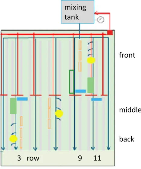
Water was pumped from a supply tank (mixing tank) to the plants via a series of tubes. Each plant had a dripper to supply water, nutrients and, during the experiment, PPP (see Figure 2-1). The drippers open due to the increased pressure each time the pump is activated. Upon opening, the water supply from each dripper was approximately 50 ml per minute. Water and dissolved substances are then taken up by the crop, and any surplus water runs to the drain tank via a drain opening on the lowest side of each slab, and via a trough and PVC pipe system. Troughs were positioned at a slope of approximately 1% to ensure fast collection of the drain water. The drain solution was pumped back from the drain tank into the mixing tank.
The mixing tank had a variable content, controlled by two sensors preventing the system from flooding and from falling dry. During the experiment, the minimum water level was set at approximately 49 cm (volume 472 L) and the maximum level at 90 cm (volume 872 L). During operation, the lower sensor triggered the automatic delivery of 400 L fresh nutrient solution to the mixing tank. The automatic water supply may be overruled; for example, prior to and during the supply of the PPP the system was switched to manual (see section 2.3).
Figure 2-1 Layout of drip irrigation and drain system of the greenhouse unit in which the experiment was conducted. Green lines indicate the water supply, red lines the drain pipes, and grey lines the slabs and the troughs.
2.2 Operational measurements during the experiment
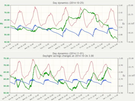
A number of measurements were performed to monitor and check crop growth, starting from the beginning of the cropping period and continued during the experiment. Measurements of radiation, temperature, water content of the slabs and electrical conductivity were logged every 5 minutes. Figure 2-2 gives an example of the measurements. During the experiment, water supply to the crop was automatically supplied between 10.00 and 15.00, based on the water requirement of the crop as calculated from measured radiation and a target drain ratio (35% of the supplied water). Cumulative radiation triggered activation of the water pump and water supply for a fixed duration of 2.5 minutes. Each time water is supplied, the water content of the slabs rises
(Figure 2-2). After each event, the water content drops due to water uptake by the crop and drainage to the troughs. Drainage lags behind water supply; usually no drainage was observed after the first water supply of the day, and none to little drainage after the second water supply. Drainage was measured occasionally during the experiment, not continuously (see Table 2-1); if not measured, the target value is given. Events preceding the application of the PPPs may have affected
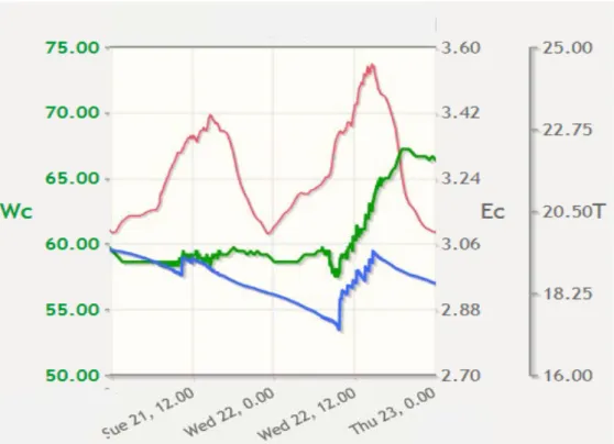
experimental conditions during the experiment. An example is that the water supply was discontinued the day before the application of the PPPs in order to lower the water content of the slabs, which is prescribed in the ‘Druppelprotocol (drip application protocol)’1. For this reason, information on water management prior to application is included. Figure 2-3 shows two days of the data given in Figure 2-2 in more detail: the day before and the day of the application of the PPPs. The watering regime was switched to manual control on 21 October, the day 1 ‘Druppelprotocol’ is the guideline for applying PPP with drip irrigation in soilless cultivation.
before the PPPs were applied to the system. After 12.00, no water was provided until the application of the PPPs on 22 October. The effect is visible in Figure 2-2; the water content drops to 53%, about 5% lower than the minimum water contents in the previous period.
The first watering event of 22 October lasted 6 minutes, where 74 L of the PPP containing solution was applied in one event. After this, the mixing tank was emptied to discard surplus PPP solution, and refilled with fresh nutrient solution to the maximum level, i.e. 872 L. The water supply was switched to the automatic position after this event, however the fourth watering event was manually forced. The following day, the first watering event was also manual; for unknown reasons it was not started automatically.
The water content of the slabs increased during the application of the PPPs, but remained below the minimum values observed the days before. No drainage was observed during and shortly after this event and also not after the following watering event. After the second watering event, a small amount of drainage was observed, but not everywhere in the system. After the next watering event, some drainage was observed at all observation points (see Figure 2.4 for the location of the sampling and observation points in the system). The drainage amounts were considered too low, which led to the manually forced water supply. The volumes of applied water were registered daily on a computer (Table 2-1).
Figure 2-2 Data from the data logger in the slabs from 19 October to 2
November. WC=water content (%, blue lines, left axis), T=temperature (°C, red lines, 2nd right axis), EC= electric conductivity (mS/cm, green lines, 1st right axis). Note the difference in scale between upper and lower panel for EC.
Figure 2-3 Data from the data logger in the slabs for 21 and 22 October. WC=water content (%, blue, left axis), T=temperature (°C, red, 2nd right axis), EC= electric conductivity (mS/cm, green, 1st right axis).
Table 2-1 Details on the daily water supply during the experimental period.
date volume of water (L) number of watering events drain (%)
20 October 259 7 40 21 October 74 2 6 22 October 259 7 15 23 October 222 6 15 24 October 296 8 31 25 October 444 12 35# 26 October 444 12 35# 27 October 518 14 35# 28 October 444 12 27 29 October 444 12 35
# estimated value; missing information prevented accurate calculation.
Temperature is important as it may influence the behaviour of the substances in the system. Temperature was recorded during the entire season, thus also during the experiment (see Figure 2-2 and Figure 2-3). The temperature varied between approximately 19 and 25 °C.
2.3 Application of the plant protection products
The experiment was performed using three PPPs: Paraat, Luna and Admire with active substances dimethomorph, fluopyram and
imidacloprid, respectively. Label instructions on the dosage of these PPP are given in Appendix 1. The weighed amounts of the PPPs and nominal concentrations in the mixing tank are given in Table 2.2. In addition to the three PPPs, a tracer (Fe-EDDHA, 40 mmol/l) was added so that the movement of the solution in the system could be followed visually. Fe-EDDHA is readily taken up by plants and therefore cannot be considered a quantitative tracer.
The PPP were applied on 22 October at 10.00. The required amounts of the three PPPs were determined, added to 2 L water and thoroughly mixed. The mixture was added to the mixing tank containing nutrient solution to reach a total volume of 166 L and thoroughly mixed. The PPP were applied by drip irrigation to the crop. The pump was activated manually and run for 6 minutes. In this way, 74 L of the solution was pumped to the cucumber plants and the rest was discarded by draining the mixing tank. Hereafter, the mixing tank was filled with fresh nutrient solution and the system was reset to automatic application.
Table 2-2 Applied masses of plant protection products, nominal concentrations of the active substances (a.s.) in the mixing tank (MT), and solubility. The nominal concentrations were calculated from the weighed masses and the batch volume. The applied amounts were calculated from the volume supplied to the system (74 L).
PPP active
substance applied mass a.s. (mg) concentration nominal a.s. (mg/L) solubility a.s. (mg/L) Paraat dimethomorph 8360 113 47.2, 10.7# Luna fluopyram 2270 30.7 15 Admire imidacloprid 1120 15.1 613 # solubility for E and Z isomers respectively
2.4 Sample collection and analyses
Samples were collected between 22 October and 28 October 2014: • On 22 October, prior to application of the PPP, samples were
taken (in duplicate) from both the mixing tank and the drain water tank to establish background concentrations.
• Samples were taken from the mixing tank directly after preparing the PPP-solution, and again after the PPPs were supplied to the cultivation.
• During application, samples were taken from the drippers at three locations in the greenhouse unit, positioned close to the yellow dots in Figure 2-4.
• On 22 October, following the primary application of PPPs, samples were taken at the same locations during the first three watering events and during the last watering event of the day. Replicates were taken when possible. Immediately after taking samples from the drippers, samples were taken from the drain water (blue rectangles in Figure 2-4), when drainage occurred. • On the following days, samples were taken at the same locations,
All samples were transferred into dark green 1 L glass bottles and sent to a commercial laboratory where they were analysed for the three substances.
Figure 2-4 Sampling locations in the greenhouse unit. The yellow dots indicate the position of the sampled drippers. Drainage samples were collected at the blue rectangles (troughs in rows 3, 9 and 11).
2.5 Analytical results
Samples were brought to the laboratory and analysed for the active substances of the three PPPs. Selected samples were also analysed for the Fe content; elevated concentrations were due to the use of the FeEDDHA colour tracer. The active substance of Paraat is dimethomorph: a mixture of the isomers E-dimethomorph and Z-dimethomorph. The laboratory did not distinguish between the two isomers; therefore, total dimethomorph contents were used for the interpretation of the
experiment.
Background concentrations of the active substances were low, but all three substances were found in the nutrient solution and in the drain water sampled prior to application of the PPPs (Table 2-3).
mixing
tank
front
middle
back
3 row 9 11
Table 2-3 Background concentrations (μg/L) in water in the cultivation system
sampled water concentration
dimethomorph fluopyram imidacloprid mixing tank before application 0.014 0.068 0.011 0.018 0.061 0.011 fresh supply mixing tank after application 0.11 0.048 # 0.094 0.043 # drain water before application 0.025 0.076 0.033 0.03 0.064 0.022 average 0.049 0.060 0.019 # not measured
Table 2-4 lists the concentrations of the three substances in the application solution. Samples of this solution were taken in duplicate from the mixing tank at the start of the application event and from the remaining application solution following application. The remaining application solution was discarded after taking the samples, and the mixing tank was refilled with fresh nutrient solution.
Table 2-4 Concentrations (mg/L) in PPP application solution
dimethomorph fluopyram imidacloprid
before dose 1# 26 22 30
before dose 2 18 26 30
after dose 1 19 30 36
after dose 2 21 30 42
Average 21 27 34.5
# 1 and 2 are replicates
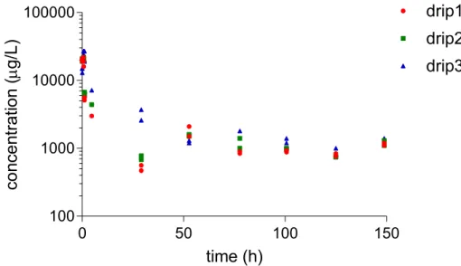
Figure 2-5 to Figure 2-6 show the concentrations in the solutions sampled from the drippers in the glasshouse unit in time, for
dimethomorph, fluopyram and imidacloprid, respectively. At the first sampling moment, concentrations are equal to the levels measured in the application solution, except for the drippers at the back which lagged behind. Concentrations decreased rapidly, as fresh nutrient solution was supplied. Later, the levels stabilise or even increase due to recirculation of the nutrient solution containing PPPs; from the fourth watering event on October 22 onwards (see Appendix 3).
Figure 2-5 Dimethomorph concentrations in samples taken from the drippers. Drippers 1, 2 and 3 are positioned in the front, middle and back of the unit respectively. Note the logarithmic scale of the Y-axis. Application of substance is at t=0 h.
Figure 2-6 Fluopyram concentrations in samples taken from the drippers. Drippers 1, 2 and 3 are positioned in the front, middle and back of the unit respectively. Note the logarithmic scale of the Y-axis. Application of substance is at t=0 h.
0
50
100
150
10
100
1000
10000
100000
time (h)
co
nc
en
tra
tio
n
(µ
g/
L)
drip1
drip2
drip3
0
50
100
150
100
1000
10000
100000
time (h)
co
nc
en
tra
tio
n
(µ
g/
L)
drip1
drip2
drip3
Figure 2-7 Imidacloprid concentrations in samples taken from the drippers. Drippers 1, 2 and 3 are positioned in the front, middle and back of the unit respectively. Note the logarithmic scale of the Y-axis. Application of substance is at t=0 h.
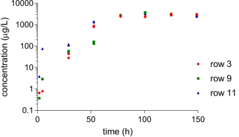
Figure 2-8 to Figure 2-10 show concentrations of dimethomorph, fluopyram and imidacloprid in the water draining from the slabs. The first moment drain water appeared from all slabs was after 3.15 h (3rd
watering event after application of the PPPs, but the volume was too low to take duplicate samples). Concentrations in this drain water were at background level. Concentrations increased more rapidly in the front end of the greenhouse unit than in the middle and the back.
Concentrations of all three substances increased up to three to four days after the application, depending on the substance.
Figure 2-8 Dimethomorph concentrations in samples taken from the troughs. Row 11 is in the front of the greenhouse unit, row 9 in the middle and row 3 in the back. Note the logarithmic scale of the Y-axis.
0
50
100
150
10
100
1000
10000
100000
time (h)
co
nc
en
tra
tio
n
(µ
g/
L)
drip1
drip2
drip3
0
50
100
150
0.1
1
10
100
1000
10000
time (h)
co
nc
en
tra
tio
n
(µ
g/
L)
row 3
row 9
row 11
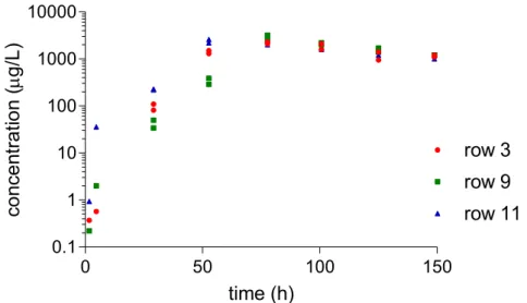
Figure 2-9 Fluopyram concentrations in samples taken from the troughs. Row 11 is in the front of the greenhouse unit, row 9 in the middle and row 3 in the back.
Figure 2-10 Imidacloprid concentrations in samples taken from the troughs. Row 11 is in the front of the greenhouse unit, row 9 in the middle and row 3 in the back.
0
50
100
150
0.1
1
10
100
1000
10000
time (h)
co
nc
en
tra
tio
n
(µ
g/
L)
row 3
row 9
row 11
0
50
100
150
0.1
1
10
100
1000
10000
time (h)
co
nc
en
tra
tio
n
(µ
g/
L)
row 3
row 9
row 11
3
Adaptations to the model and generation of input files
In GEM (Wipfler et al. 2015, van der Linden et al. 2015), three models are used to simulate the fate and behaviour of substances in substrate cultivations. The WATERSTREAMS model (Voogt et al. 2012) simulates the water flows in the greenhouse including the water supply to the crop and the amounts discharged from the system to the surface water. The substance emission model uses the water flows generated by the WATERSTREAMS model and calculates the behaviour of a substance in the greenhouse system, including concentrations of the substance in various tanks, uptake by the crop, and the discharge to the surface water. TOXSWA calculates the fate and behaviour of the substance in the ditch into which the water leaving the greenhouse is discharged. The results are further used in the authorisation procedure.
This report only addresses the second model; the Substance Emission Model (SEM). In order to interpret the results of the experiment and identify recommendations for a future validation experiment, the model had to be adapted to mimic the experimental set-up (see section 3.1). During the experiment, several water flows were recorded and these were transferred into input files for the Substance Emission Model. Thus the measured water flows in this case replace the water flows calculated with the WATERSTREAMS model (see section 3.2). During the
experiment, no discharge to surface water occurred.
Major assumptions in SEM are that the solution in the various parts of the system is well-mixed, that sorption in substrate systems with stone wool is absent, and that the dissipation of the substance is by plant uptake and degradation in the water phase.
3.1 Adaptations of the substance fate model
GEM scenarios were developed to resemble greenhouse conditions typical of current growing conditions. The scenarios are for a production area of 1 ha, a fair estimate of net production areas within one greenhouse in the Netherlands. The schematisation of the greenhouse in GEM is different from the lay-out of the experiment in the greenhouse unit in Bleiswijk. The greenhouse unit production area was much smaller, fewer tanks were used, and the relative sizes of the tanks were different. The principle of the growing system, however, can be regarded as identical to the
principle in the GEM scenarios for crops grown on substrate slabs, i.e. the crop received its nutrient solution from the mixing tank and the surplus water drained to the drain water tank.
The mixing tank in the experiment combined the functions of the drain water tank, the clean water tank, and the mixing tank in the GEM scenarios. This – triple – function required the mixing tank to be
relatively large, much larger than its relative size in the GEM scenarios. Figure 3-1 presents a simplified schema of the experimental system.
Figure 3-1 Backbone schematisation of the experimental system for use in a simulation package. Water flows are indicated with arrows. MT=mixing tank, Cult= cultivation consisting of slabs including the plant roots, Crop= stems, leaves and fruits of a greenhouse crop, DWT=drain water tank.
The following section addresses the most important assumptions and processes pertinent to and occurring in the system. A full description is provided by Van der Linden et al. (2015). One of the most important concepts in the Substance Emission Model for soilless cultivation in GEM is that the system can be described as a series of connected tanks with a known constant volume of water, which is assumed to be perfectly mixed in each tank. The concentration of a substance in a tank is determined from inflow and outflow, and processes taking place in the tank. There is no check in the model on whether the solubility of the substance is exceeded.
Degradation in all tanks is described according to a first-order process: 𝑑𝑑𝑑𝑑
𝑑𝑑𝑑𝑑 = 𝑓𝑓𝑇𝑇 𝑘𝑘𝑑𝑑𝑒𝑒𝑒𝑒 𝑑𝑑 where
C concentration of the substance, μg/L
fT factor, -, for the influence of temperature on the degradation, fT is
a function of time and may be different for each tank kdeg first-order degradation rate coefficient, d-1
with
𝑘𝑘𝑑𝑑𝑒𝑒𝑒𝑒 =𝐷𝐷𝐷𝐷𝐷𝐷𝐷𝐷ln (2)
50 where
DegT50 half-life of the substance, d, at reference conditions. The
half-life may be specific for each tank.
The half-life may be specific to a tank and its operating conditions. For example, the half-life can be different in a disinfection tank because of addition of a disinfectant or application of UV light. This was not tested here as there was no disinfection unit operational during the experiment.
MT Cult Crop
DWT
Evapotranspiration
Degradation is dependent on the temperature. In GEM, this influence is calculated from the Arrhenius equation:
𝑓𝑓𝑇𝑇= exp �−𝐸𝐸𝐸𝐸𝐸𝐸𝑑𝑑𝑅𝑅 �𝐷𝐷𝑡𝑡𝑡𝑡𝑡𝑡𝑡𝑡−1 − 𝐷𝐷𝑟𝑟𝑒𝑒𝑟𝑟−1�� where
Eact Arrhenius activation energy, J mol-1
R molar gas constant, 8.314 J mol-1 K-1
Ttank actual temperature in the tank, K
Tref reference temperature, usually 293.15 K (20 °C)
One dissipation process is the uptake of substances by the crop. Passive uptake along with water is assumed, but, compared to water uptake, reduced dependent on substance properties. Currently this is
implemented in GEM via the Transpiration Stream Concentration Factor (TSCF) which is calculated using Briggs’ formula (Briggs et al. 1982):
𝐷𝐷𝑇𝑇𝑑𝑑𝑇𝑇 = 0.784 × 𝐷𝐷−(log 𝐾𝐾𝑜𝑜𝑜𝑜2.44−1.78)2 where
Kow the octanol water partition coefficient, (-)
As noted earlier, GEM assumes constant water volumes for the various tanks. In the experimental situation, the water content of the mixing tank fluctuated. The mixing tank was equipped with floats which were connected to the computer. The lower float signalled the computer to deliver fresh water, while the upper float signalled the computer to stop delivery of fresh water. Additional safety floats attached to alarms, were installed, but safety levels were not breached during the experiment. The delivery of fresh water was assumed to be a pulse, so the fresh water was added instantly to the mixing tank. The added volume was assumed equal to the volume of the tank between the two floats. Float levels and the surface area of the mixing tank were used to calculate the water content of the mixing tank. The water contents of the other tanks were assumed to be constant, although in practice some variation in time was noted.
During the experiment, for practical reasons, samples were taken from the drippers delivering nutrient solution to the slabs, and from the troughs collecting the drain water returning to the mixing tank. This was accounted for by considering the tubes between the mixing tank and cultivation and the tubes and troughs between cultivation and drain water tank as separate tanks, with known (small) volumes (Figure 3-2). The model code used for the interpretation of the experiment is given in Appendix 2.
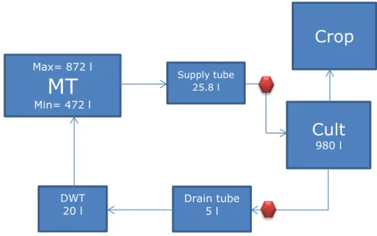
Figure 3-2 Overview of the experimental greenhouse used in the simulation model. MT= mixing tank, Cult=cultivation consisting of stone wool slabs and plant roots, Crop= plant stems, leaves and fruits. DWT=drain water tank. Supply tube and drain tube are the tube from the mixing tank to the cultivation and the troughs from the cultivation to the drain water tank, respectively. All volumes (litres) were calculated from the total length of the tubes and their inner diameters. The diamonds represent the sampling points. The volume of drain tube was not known and was estimated to be five litres.
3.2 Water input file for the calculations
From the experimental conditions, it was considered most appropriate to use an hour as basis for the input files for the calculations.
All tanks, except the mixing tank, were assumed to have constant water content over time, although some fluctuations occurred. This
assumption is equal to the approach taken in GEM in the scenarios used for the authorisation evaluations. The assumption of constant water content is poor for the drain water tank, but the volume of this tank is so small that this has little influence on the calculation results.
The volume of the mixing tank fluctuates, as fresh nutrient solution is supplied in batches triggered by the floats in the tank. The content of the mixing tank is calculated from the water flows into (drainage water and fresh water) and out of the tank (water supply to the crop). Immediately after application of the PPPs, before the first watering event, the mixing tank was filled to the maximum level. This was used as the starting volume of the mixing tank. A float at 50 cm, i.e. at a water content of 472 L, signalled the delivery of 400 L fresh nutrient solution.
The volumes of the tubes were calculated from the lengths and
diameters of the tubes present in the system. The water content of the cultivation was estimated to be 980 L. The average water content of the stone wool slabs in the first 8 days after the application of the
substances was 58% (V/V), which amounted to a water content of 900 L in the slabs. At the start of the cultivation, i.e. months before the start of the experiment, plants were transferred to the slabs in a volume of
Max= 872 l
MT
Min= 472 l Supply tube 25.8 lCrop
Cult
980 l Drain tube 5 l DWT 20 l1 L stone wool substrate. Water content of this additional substrate was unknown (not measured). For the calculations, it was assumed that the average water content was 29%, i.e. 50% of the measured water
content of the slabs. Water content was expected to be lower than in the slabs because of evaporation at the top and the vertical gully that was used to supply the solution, leading to lower water contents at the top. The water supply from the mixing tank to the crop was registered daily by the central control system. However, in practice, the water was supplied in a limited number of watering events. In each event, nutrient solution was pumped for 2.5 minutes at a constant rate, equivalent to a volume of 30.8 L (about 10% lower than indicated in Figure 2.1). The water supply per minute (12.33 L) was calculated from the measured volume supplied during application of the PPPs (74 L) and the duration of the application event (6 minutes). The starting time of each event was read from the registration of the water content of the slabs; the water content increased immediately at each watering event. Each watering event was assigned to the nearest hour.
Surplus water drains from the substrate slabs under gravity. Usually, drainage starts each day either during or immediately after the second watering event and occasionally during or after the third watering event. Because of water uptake by the crop between the last watering event on the previous day and the first watering event on the current day, there is a shortage, and the surplus of the first watering event counterbalances this. Thus, the number of drainage periods on each day is mostly equal to the number of watering events minus one.
The drainage situation on the day of application was different from the other days. Due to the application of the ‘Druppelprotocol (Drip
application protocol)’, the water content in the slabs was relatively low at the moment of application of the PPP. The volume of water used for applying the PPP, 74 L, was not sufficient to fully replenish this lower level, resulting in a low overall drainage percentage. The drainage pattern was closely followed and the observed pattern used to construct the drainage file for this day.
The volumes of water draining from the slabs were measured for a part of the experimental period only and assigned to the appropriate
drainage periods. For the other periods, i.e. periods without measured drainage volume, it was assumed that 35% drainage was achieved (approximately the target value).
Temperatures were recorded at three different locations in the slabs. The average temperature as a function of time was used in the calculations.
4
Interpretation of the concentrations
4.1 Applied amounts of PPP
Nominal concentrations in the application solution differ from measured concentrations and therefore there is uncertainty with respect to the amounts effectively supplied to the system (see also Table 4-1):
• For dimethomorph, the nominal concentration (113 mg/L) was approximately five times the measured concentration (average of measurements in the application solution before and after the application is 21.3 mg/L). The reason for this difference may be due to exceeding the solubility of dimethomorph in water. The solubilities of the E- and the Z-isomer are 47.2 and 10.7 mg/L respectively, so below the nominal concentration.
• For fluopyram, nominal and measured concentrations in the application solution differ by approximately 10%. The average measured concentration (27 mg/L) is about twice the solubility of the substance in water (15 mg/L).
• For imidacloprid, the average measured concentration is 29.3 mg/L, which is about twice the nominal concentration.
The variation coefficients of the measurements of the concentrations in the application solution are 14%, 11% and 26% for dimethomorph, fluopyram and imidacloprid, respectively; this is high for these concentration levels.
Concentrations greater than the water solubility may be caused by formulation additives which enhance the dispersion of the substance in the application solution. Neither, the identity of the formulation
additives, nor the behaviour of these additives in the system was known. It is therefore unclear for how long and where concentrations above water solubility can occur.
Given the uncertainty in the applied amounts, two approaches were followed in the simulations (section 4.3): one in which the applied amounts were based on the measured concentrations of the PPPs (MC approach), and one in which the applied amounts were based on the nominal concentrations of the PPPs in the application solution (WA approach), i.e. concentrations derived from weighted amounts.
Table 4-1 Amounts and concentrations of PPP applied to the system. In the MC approach, the mass applied is based on the measured concentrations in the application solution. Variation coefficients are given in between brackets. In the WA approach, the mass applied is derived from the weighted amounts.
MC approach WA approach
mg mg/L mg mg/L
dimethomorph 1574 (14%) 21.3 8358 113 fluopyram 2004 (11%) 27.0 2273 30.7 imidacloprid 2172 (26%) 29.3 1123 15.1
4.2 Measured concentrations in the system
Figure 4-1 shows the averages of the concentrations of the active substances of the PPPs and their ranges in water flowing from the drippers towards the cultivation, in time. The range in concentrations was not only caused by variability due to the measurement method, but also to the response time of the drippers to changes in concentrations in the mixing tank. The drippers at the front end are closer to the mixing tank and therefore respond more quickly to changes in concentrations in the mixing tank than drippers in the middle and back. After application of the PPP solution, times for the PPP solution to arrive were 80, 130 and 190 seconds for the front, middle and back drippers respectively (see Appendix 3). The differences in response time are ignored in the figures in this report. Concentrations of all three substances declined rapidly, average concentrations at the second sampling time (t = 1 h) were at least one order of magnitude below the initial concentrations. Fresh nutrient solution replaced the contents of the tubes. The total volume of the tubes is smaller than the amount of water delivered during one watering event. However, due to the differences in response time because of the positions of the drippers in the greenhouse, a high variation in concentration was observed, especially in the first few hours after the application. Imidacloprid declined most rapidly, followed by fluopyram; dimethomorph declined most slowly. After the first few hours, the behaviour of fluopyram and imidacloprid was similar. The difference during the first few hours was possibly caused by fluopyram being slightly above its ideal solubility level. Dimethomorph declined more slowly during the first day and had a fairly constant concentration around 1 mg/L thereafter.
The lowest concentrations for fluopyram and imidacloprid were observed at t = 29.1 h. Concentrations of these two substances increased after that moment because the drainage water containing the substances was recycled to the mixing tank (see Appendix 3).
Figure 4-1 Measured concentrations of dimethomorph (D), fluopyram (F) and imidacloprid (I) in water sampled from the drippers. The error bars indicate the range of concentrations. In many cases, there is overlap in ranges observed for fluopyram and imidacloprid.
0
50
100
150
10
100
1000
10000
time (h)
co
nc
en
tra
tio
n
(µ
g/
L)
F
D
I
Concentrations of the three substances in the drain water stayed well below the solubilities. All three substances were present in the first drain water sample after application, but concentrations were at background level. The following samples had concentrations at least one order of magnitude above the background level. After the second sampling point in time, concentrations of imidacloprid increased most quickly, followed by fluopyram and dimethomorph. Concentrations of imidacloprid
declined after 53 h and those of fluopyram after 78 h. Dimethomorph concentrations increased until 78 h and stayed fairly constant thereafter.
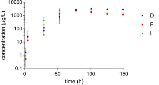
Figure 4-2 Concentrations of dimethomorph (D), fluopyram (F) and imidacloprid (I) in samples taken from the troughs. The error bars indicate the range of measured concentrations. In many cases, there is an overlap in ranges observed for the three substances, mostly for fluopyram and imidacloprid.
Figure 4-3 to Figure 4-5 show the concentrations in water sampled from the drippers and in the drain tube for the individual substances as a function of time. The concentrations in the drain tube were higher than the concentrations in the water sampled from the drippers after 29 h (imidacloprid), 53 h (fluopyram) and 78 h (dimethomorph). The lower concentrations in water sampled from the drippers, as compared to the concentrations in the drain tube, may have been caused by both dilution with fresh water added to the mixing tank (see Figures 3-1 and 4-6) and the uptake factor (TSCF) of the substances being less than one.
However, the fact that the concentrations of the three substances in the water draining from the cultivation system in the second half of the experiment were consistently at least a factor two higher than in the water flowing towards the cultivation system, can only be explained by the TSCF being substantially less than one.
0
50
100
150
0.1
1
10
100
1000
10000
time (h)
co
nc
en
tra
tio
n
(µ
g/
L)
F
I
D
Figure 4-3 Measured dimethomorph concentrations in water sampled from the drippers (D_in) and water sampled from the troughs (D-out). The error bars indicate the range of measured concentrations.
Figure 4-4 Measured fluopyram concentrations in water sampled from the drippers (F_in) and water sampled from the troughs (F_out). The error bars indicate the range of measured concentrations.
0
50
100
150
0.1
1
10
100
1000
10000
time (h)
co
nc
en
tra
tio
n
(µ
g/
L)
D_out
D_in
0
50
100
150
0.1
1
10
100
1000
10000
time (h)
co
nc
en
tra
tio
n
(µ
g/
L)
F_in
F_out
Figure 4-5 Measured imidacloprid concentrations in water sampled from the drippers (I_in) and water sampled from the troughs (I_out). The error bars indicate the range of measured concentrations.
4.3 Simulations and comparison with measurements
4.3.1 Model input parameters and simulated water balance
Measurements showed that all three substances were present in the system before the PPPs were applied. As these background concentrations were low, at least four orders of magnitude below initial concentrations in the mixing tank, they were assumed zero in the calculations.
The Substance Emission Model modified for this experiment requires as input: the lay-out of the experiment, the water flows between the different units as a function of time (see previous chapters), the applied amount of PPP and the temperature as a function of time and place (see chapter 2). It was assumed that the measured temperatures in the slabs also represent temperatures of the other elements.
The following dissipation processes are included in the SEM model for drip-application: plant uptake, degradation in the water in the various tanks, and discharge from the system. No discharge occurred during the experiment. The reference half-lives of the substances, i.e. the half-life in water at 20 °C, were assumed applicable to the whole system. However, in absence of information on degradation of the substances in the system, in most of the simulations a reference half-life of 1000 days (24000 h) was assumed for all three substances, indicating negligible degradation during the experimental period. A default Arrhenius
activation energy of 65400 J/mol was assumed for all three substances. When the degradation is negligible, the value chosen for the activation energy has a negligible effect on the calculated concentrations.
SEM assumes passive uptake of the substances by plants, but influenced by the octanol water partition coefficient according to Briggs et al.
(1982). Octanol water partition coefficients were taken from the dossiers (see Appendix 4). The calculated TSCF values were 0.58 (dimethomorph E-isomer), 0.54 (dimethomorph Z-isomer), 0.30 (fluopyram) and 0.43
0
50
100
150
0.1
1
10
100
1000
10000
time (h)
co
nc
en
tra
tio
n
(µ
g/
L)
I_in
I_out
(imidacloprid). The expected plant uptake is thus relatively high for dimethomorph and relatively low for fluopyram. All three TSCF values indicate that relative enrichment of the substances in the cultivation will occur, in increasing order dimethomorph, imidacloprid and fluopyram. Figure 4-6 shows the cumulative water fluxes from the mixing tank to the cultivation, from the cultivation to the crop, from the cultivation back to the mixing tank, and the water contents of the mixing tank, across time. The cumulative fluxes and the fresh water supply were calculated from the information given in section 3.2. Total fresh water supply to the mixing tank was calculated at 1200 L, i.e. 3 times 400 L after 48 h, 92 h and 121 h. The total water delivery to the cultivation system was 2230 L plus the volume of the application solution.
Evaporation amounted to 1592 L, and 658 L drained from the cultivation back to the mixing tank.
As can be seen in Figure 4-6, the movement of water occurs during day time, and no water movement is simulated during the night (horizontal line segments). After approximately 92 h, a volume equal to the
average wet contents of the slabs is supplied to the slabs. In the second half of the experiment, growing conditions were better than in the first half, resulting in a higher water demand of the crop. The pattern of water flows influences simulated concentrations of the PPPs (see following sections); at night, no water flows in the tubes and troughs.
Figure 4-6 Calculated cumulative water fluxes (left axis) and water content of the mixing tank (right axis) during the experiment. Purple: water supply to the cultivation system, red: water taken up by the crop, green: water drained from the cultivation system, black: water content of the mixing tank.
Due to the uncertainty about the amounts of PPP applied to the system (section 4.1), two approaches were followed for the simulations. In the first (approach MC), the amounts of substances applied were calculated from application volume and the measured concentrations in the
application solution. In the second (approach WA), the amounts of substances applied were calculated from the application volume and the
0
50
100
150
0
500
1000
1500
2000
2500
400
600
800
1000
time (h)
cu
m
ul
at
iv
e
flu
x
(L
)
vo
lum
e (
L)
nominal concentrations in the application solution. Results of both approaches are discussed in the following sections.
4.3.2 Dimethomorph
Figure 4-7 shows measured (dots) and simulated (solid lines)
dimethomorph concentrations in the nutrient solution sampled from the water flowing towards the cultivation, in time. The model simulates a drop in the concentration of approximately three orders of magnitude in the first few hours after the start of the experiment. The water in the tubes is refreshed several times with water containing background concentrations. The drop in measured concentrations is less than one order of magnitude. The differences between calculated and measured concentrations are largest at the last sampling time on the day of application, i.e. 5 h after the start of the experiment.
On the second day, simulated dimethomorph concentrations in the tubes started to increase. This is due to incoming water with higher
concentrations than the background concentrations, as a result of drainage water containing dimethomorph being returned to the mixing tank. Concentrations increase during the day on days 1 to 3, after which the concentrations level at approximately 0.3 mg/L (approach MC) respectively 1.0 mg/L (approach WA). In contrast, measured
concentrations continued to decline for the first 4 days of the experiment, reaching the lowest concentration of approximately 1 mg/L. Hardly any influence of the water dynamics could be observed in the measurements. From 78 h after the start onwards, simulated concentrations according to the WA approach are close to the ranges observed in the measurements. The difference between measured and simulated concentrations in the first few days cannot be explained with the available information. A possibility is that some dimethomorph settled in solid form on the wall of the tubes and was released back into the solution once the
concentrations dropped below solubility.
Dimethomorph dissipated in the simulations from the system almost exclusively via uptake by the crop. At the end of the experiment, 54% of the applied amount was taken up by the crop. At the same time, only 0.36% of the applied amount had degraded. The negligible effect of degradation was expected because of the assumed dimethomorph half-life of 1000 days. The potential effect of degradation is discussed in section 4.3.4.
Figure 4-7 Measured (dots) versus calculated (lines) dimethomorph
concentrations in water sampled from the drippers. The bars indicate the range in measured concentrations. Red line: MC approach, blue line: WA approach.
Figure 4-8 gives measured (dots) and simulated (solid lines) dimethomorph concentrations in the solution draining from the cultivation, in time. The model simulates a fast rise in concentrations shortly after the start of the experiment, from the moment draining starts. Measured concentrations also increased shortly after the start of the experiment, but slower than the simulated concentrations. In the MC approach, simulated concentrations are above measured concentrations for the first two days, and below measured concentrations afterwards. The pattern of measured concentrations was not observed in the simulations. Simulated concentrations are above measured
concentrations in the WA approach for the first three days, but match afterwards. The WA approach appears to reflect measurements better than the MC approach.
0
50
100
150
0.001
0.01
0.1
1
10
time (h)
co
nc
en
tra
tio
n
(m
g/
L)
Figure 4-8 Measured versus calculated dimethomorph concentrations in water sampled from the troughs. The bars indicate the range in measured
concentrations. Red line: MC approach, blue line: WA approach.
4.3.3 Fluopyram
Figure 4-9 gives measured (dots) and simulated (solid lines) fluopyram concentrations in the nutrient solution flowing towards the cultivation, in time. As seen for dimethomorph, the model simulates a drop in the concentrations of approximately three orders of magnitude in the first few hours. The water in the tubes is refreshed several times with water not influenced by added PPPs, as drainage has not yet occurred. The drop in measured concentrations is about a factor 20, depending on the location in the system (see also Figure 2-6).
On the second day, simulated concentrations in the tubes start to rise. This is due to incoming water with higher concentrations than the background as a result of drainage water containing fluopyram being returned to the mixing tank. The simulated concentrations on the second day are in the range of the measured concentrations. Simulated concentrations rise slightly after the second day, except shortly after fresh water is added to the system at approximately 2, 4 and 5 days after the start of the experiment (see also Figure 4-6). In general, measured and simulated concentrations are similar; simulation results are within the range of the measurements in three of six sampling times after the first day. Differences between the two approaches, MC and WA, are small; initial amounts differ by 13%.
Like dimethomorph, fluopyram dissipates from the system in the
simulations almost exclusively via uptake by the crop. At the end of the experiment, 34% of the applied amount is taken up by the crop. At the same time, only 0.42% of the applied amount had degraded. The negligible effect of degradation was expected because of the assumed half-life of fluopyram of 1000 days. The potential effect of degradation is further discussed in section 4.3.4.
0
50
100
150
0.001
0.01
0.1
1
10
time (h)
co
nc
en
tra
tio
n
(m
g/
L)
Figure 4-9 Measured (dots) versus calculated (line) fluopyram concentrations in water sampled from the drippers. The bars indicate the range in measured concentrations. Red line: MC approach, blue line: WA approach.
Figure 4-10 gives measured and simulated fluopyram concentrations in the solution draining from the cultivation, in time. The model simulates a fast rise in concentrations shortly after the start of the experiment, from the moment drainage starts. Measured concentrations also rise shortly after the start of the experiment, but slower than the simulated concentrations. Simulated concentrations are above measured
concentrations during the first and second day, but are within the range of measured concentrations on three out of five sampling times
afterwards. In the drain water, differences between both approaches, MC and WA, are also small.
Figure 4-10 Measured (dots) versus calculated (line) fluopyram concentrations in water sampled from the troughs. The bars indicate the range in measured concentrations. Red line: MC approach, blue line: WA approach.
0
50
100
150
0.001
0.01
0.1
1
10
TIME
co
nc
en
tra
tio
n
(m
g/
L)
0
50
100
150
0.001
0.01
0.1
1
10
TIME
co
nc
en
tra
tio
n
(m
g/
L)
4.3.4 Imidacloprid
Figure 4-11 shows measured (dots) and simulated (solid lines)
imidacloprid concentrations in the nutrient solution flowing towards the cultivation, in time. The model simulates a drop in the concentration slightly lower than three orders of magnitude in the first few hours. The water in the tubes is refreshed several times with water not influenced with added PPPs, as drainage has not yet occurred. The drop in measured concentrations is about two orders of magnitude depending on the
location in the system (see also Figure 2-7), so slightly lower than
simulated. On days 2–4, simulated concentrations in the tubes are within the range observed in the measurements, in both the MC and the WA approach. Later on in the experiment, simulated concentrations are slightly below observed concentrations in both approaches, but in the MC approach they are closer to the measurements than in the WA approach. As with dimethomorph and fluopyram, imidacloprid dissipates from the system almost exclusively via uptake by the crop. At the end of the experiment, 45% of the applied amount is taken up by the crop. At the same time, only 0.38% of the applied amount has degraded. The negligible effect of degradation was expected because of imidacloprid’s assumed half-life of 1000 days. The potential effect of degradation is discussed in section 4.3.4.
Figure 4-11 Measured (dots) versus calculated (line) imidacloprid concentrations in water sampled from the drippers. The bars indicate the range in measured concentrations. Red line: MC approach, blue line: WA approach.
Figure 4-12 shows measured (dots) and simulated (solid lines)
imidacloprid concentrations in the solution draining from the cultivation, in time. As for dimethomorph and fluopyram, the model simulates a fast rise in concentrations shortly after the start of the experiment, from the moment draining starts. Measured concentrations also rise shortly after the start of the experiment, but slower than the simulated concentrations. Simulated concentrations are above measured concentrations in the first and second day for both approaches. After the second day, simulated concentrations are similar to the ranges of the measurement on 4 out 5 days (MC approach) but slightly below measured concentrations at all
0
50
100
150
0.001
0.01
0.1
1
10
time (h)
co
nc
en
tra
tio
n
(m
g/
L)
sampling times in the WA approach. The MC approach appears to reflect measurements better than the WA approach.
Figure 4-12 Measured (dots) versus calculated (line) imidacloprid concentrations in water sampled from the troughs. The bars indicate the range in measured concentrations. Red line: MC approach, blue line: WA approach.
4.3.5 Influence of TSCF and DegT50
Simulations in the previous sections used TCSF values based on octanol-water partition coefficients using the Briggs formula (Briggs et al. 1982). For fluopyram, the calculated TSCF is 0.3. Figure 4-13 shows the
influence of varying the TSCF from 0 to 1 on simulated concentrations in nutrient solution flowing towards the cultivation and Figure 4-14 on simulated concentrations in the drain tubes. Higher TSCF values result in more uptake of substance by the crop and therefore lower
concentrations in the system. The simulations suggest that a value in the low range is more in line with the observations. The experiment should have been extended in time to determine an appropriate value for the TSCF. It is likely that the same conclusion can be derived for dimethomorph and imidacloprid, should those simulations be performed.
0
50
100
150
0.001
0.01
0.1
1
10
time (h)
co
nc
en
tra
tio
n
(m
g/
L)
Figure 4-13 Influence of TSCF on simulated fluopyram concentrations in the nutrient solution flowing towards the cultivation. TSCF increases from 0 (top line) to 1 (bottom line) with increments of 0.1. The dots are the measured concentrations.
Figure 4-14 Influence of TSCF on simulated fluopyram concentrations in water draining from the cultivation. TSCF increases from 0 (top line) to 1 (bottom line) with increments of 0.1. The dots are the measured concentrations. Applied amount according to the MC approach.
0
50
100
150
0.0
0.2
0.4
0.6
0.8
1.0
time (h)
co
nc
en
tra
tio
n
(m
g/
L)
0
50
100
150
0
1
2
3
4
time (h)
co
nc
en
tra
tio
n
(m
g/
L)
The simulations in the previous sections assumed negligible transformation of the substances in the system; DegT50s were assumed to be 1000 d = 24000 h. Figure 4-15 and Figure 4-16 show the effect of shorter half-lives on simulated concentrations. With a half-life of 12 h, a substance
disappears almost completely from the system within 6 days, i.e. the duration of the experiment. Results from simulations with half-lives above 200 h cannot be distinguished from each other in the graphs; the influence of degradation is negligible. The measurements indicate that degradation was indeed negligible during the experiments. Simulations (not presented) indicated that degradation is also negligible for imidacloprid. Similar simulations for dimethomorph were not performed.
Figure 4-15 Influence of DegT50 on simulated fluopyram concentrations in nutrient solution flowing towards the cultivation. DegT50 decreases from 24000 h (top line) to 12 h (bottom line). The dots are the measured concentrations. Applied amount according to the MC approach.
Figure 4-16 Influence of DegT50 on simulated fluopyram concentrations in the drain tubes. DegT50 decreases from 24000 h (top line) to 12 h (bottom line). The dots are the measured concentrations. Applied amount according to the MC approach. 0 50 100 150 0.00001 0.0001 0.001 0.01 0.1 1 10 time (h) co nc en tr at io n (m g/ L) 0 50 100 150 0.00001 0.0001 0.001 0.01 0.1 1 10 time (h)