1
PBL WORKING PAPER 11 May 2013
Consumer city or production city? Market
areas and density effects in the Netherlands
THOMAS DE GRAAFFa,b and OTTO RASPEaa PBL Netherlands Environmental Assessment Agency, P.O. Box 30314, 2500 GH, The Hague, The Netherlands
b Department of Spatial Economics, Vrije Universiteit Amsterdam, De Boelelaan 1105, 1081 HV, Amsterdam, The Netherlands
Abstract
Using detailed Dutch grid cell data we investigate the elasticity between population and amenities in the Netherlands for both employment and number of establishments. We do so by applying various econometric techniques (including fixed effects and a multilevel modeling approach, where the various levels represent grid cell and municipality levels). We find that municipalities differ in their elasticities between population and amenities, but differ significantly more across types of amenities. Moreover, elasticities are significantly higher for employment figures than for the number of establishments, which might point to a domination of internal scale economies over external scale economies.
Keywords: Amenities, multilevel modeling, economies of urbanisation JEL-classification: R12, R15
2
1 Introduction
In his influential 2001 paper (and later in his 2006 paper) Edward Glaeser argued that the recent urban resurgence was to a large extent caused by so-called consumer externalities (Glaeser et al., 2001 and Glaeser and Gottlieb 2006). That is, when cities are becoming larger they are able to offer a larger variety of facilities and amenities which is valued by the public at large.1 This entails that larger cities should show more facilities and amenities per capita than smaller cities and that this increase in variety and options is valued positively by the population. If so, then this would have large consequences for cost-benefit analyses of large housing projects. Namely, if the population of a city would increase then this would have positive effects for both the existing and the new population, due to these so-called consumer externalities. Unfortunately, there is yet little insight in the empirical relation between population and size and number of amenities in the Netherlands.
In this paper, we therefore look at the empirical relation between amenities and population in the Netherlands. This research focuses on two aspects. Firstly, we investigate to what extent size and number of amenities change if population changes and whether there are structural differences between types of amenities and across municipalities. Secondly, we are interested in the differences between amenities measured by the number of employees and the number of establishments. This distinction is crucial to determine whether we deal with internal or external economies of scale. Only the latter can be associated with consumer externalities.
This paper falls in a literature that deals with one of the most important recent spatial phenomena: namely, the resurgence of cities’ attractiveness. Since a few decades, most cities in the western world have positive net inflows of migrants again instead of positive net outflows (see, e.g., de Groot et al., 2010). Thus, on average, it seems that cities offer relatively more advantages than disadvantages—or, the positive externalities (such as more amenities and larger job-markets) have started to dominate the negative externalities (such as crime and congestion).2
These positive agglomeration externalities have been researched from two sides: namely, from the production and from the consumption side. The production side shows relatively moderate effects of population increase with elasticities between population and production roughly between 0–5%.3 The externalities on the consumer side assume that residents appreciate the city more because the relative oversupply of amenities, such as shops,
1 In addition, clustering of facilities and amenities decrease search and travel costs for employers, employees and customers.
2 See, for a general discussion of agglomeration externalities, inter alia, Krugman (1991), Fujita et al. (1999) and Fujita and Thisse (2002).
3 These elasticities can be found in, inter alia, Combes (2000), Duranton (2003), Duranton and Overman (2005), Combes et al. (2008), Melo et al. (2010), Puga (2010), Combes et al. (2011) and Baum-Snow and Pavan (2012), where the more recent publications find the lowest elasticities.
3
museums, restaurant, etc.4 Obviously, both the production and the consumption side are very closely related with each other (cf., Roback, 1982).
On smaller spatial scales—apart from the somewhat more socio-geographical market area literature— there is only a small literature that deals with the relation between population and amenities. This paper adds to this literature by investigating the elasticity between population and amenities in the Netherlands for both employment and number of establishments using detailed Dutch grid cell data.
In general we find that municipalities differ in their elasticities between population and amenities, but differ significantly more across types of amenities. Moreover, elasticities are significantly higher for employment figures than for the number of establishments, which might point to a domination of internal scale economies over external scale economies. Thus, evidence for consumer externalities is limited and depends as well on the specific municipality and the type of amenity.
The remainder of this paper is structured as follows. In the next section, we deal with the empirical and theoretical literature concerning market areas. Thereafter, in section 3 we give an exposition of the data we use. Section 4 deals with the empirical implementation and findings. In section 5 we concisely discuss how our findings relate to the literature concerning urban externalities and the final section concludes.
2 Market areas: theoretical and empirical background
As indicated above, we are primarily interested in the relation between the supply of specific amenities and the size of the population (or the density within an area). Specifically: does the number or size of amenities grow relatively more when population grows. If this is namely the case, then this would point to externalities—whether from the Marshallian-Arrow-Romer type (the localization economies) or from the Jacobs type (urbanization economies), depending on whether the size or the number of amenities grows (O’Sullivan, 2003). Within the context of market areas there is already a large (regional science) literature that deals with estimating these market areas.
This literature starts with Berry and Garrison (1958) and Beckman (1958). The former focuses on the question how to deal with the critical size of market areas in order to profitably operate a facility and the latter begins his paper with the following remark:
“In the classical tradition of location theory let us assume a homogeneous plain over which all resources are distributed at a uniform density. How can this uniformity generate a discrete and highly stratified network of cities? This has been the central problem in Lösch’s theory of location. Of course, the ultimate answer lies in the indivisibility of certain economic operations and the resultant economies of scale in performing the production and distribution functions of cities (page 243).”
4 This is a considerable smaller literature; for some articles, see, inter alia, Henderson (1982), Glaeser et al. (2001) and Glaeser et al. (2006).
4
The research question concerning the relation between population and amenities has primarily stimulated a discussion in the regional science literature (see, inter alia, Shonkwiler and Harris, 1996, Wensley and Stabler, 1998, Henderson et al., 2000, and Munshinksy and Weiler, 2002) but is as well addressed in the urban economics literature (see, e.g., Ades and Glaeser, 1995). The primary aim of this literature is to explain the number of amenities by the size of the population.
As the above quotation shows clearly the theoretical framework of market areas is associated with the early work of Christaller (1996) and Lösch (1954) (see as well, O’Sullivan, 2003). Building on this, the size of market areas is commonly determined by the following equation:
𝑀 =𝑑 × 𝑒,𝑞 (1)
where M denotes the size of the market area for a firm, q the equilibrium output of that firm,
d the population density and e the demand per capita for the products of that firm. A crucial
assumption for equation (1) is that the price of a product is determined by the sum of the production price (the mill price) and the transportation costs (whether these are borne by the consumers of the firms is irrelevant for the equilibrium outcome).
Conditional on the production structure, market areas will thus shrink when population density and per capita demand increases. Namely, more firms (or, as in our case, amenities) will enter the market. Thus, the number of amenities will increase as well as the total employment within a particular sector. If production is associated with internal economies of scale, then equilibrium output, q, will increase and, due to the economies of scale, prices will go down. The latter spurs again per capita demand, e. Which one will prevail is an empirical question, but economies of scale are usually associated with larger market areas. A similar argument can be made for the effect of smaller transportation costs. These will lead to again a larger equilibrium output, q, and higher per capita demand,
e. And, again, usually the former dominates the latter, thus leading to larger market areas.
If there are external economies of scale (in the form of consumer externalities), then a larger customer base is attracted when there is a larger amount or variety of amenities. Note that this larger customer base can also exists of visitors or tourists. This means that d increases, while—although transportation costs in the form of search costs decreases—the firms cannot benefit as much as they want from internal economies of scale. Namely, customers are more attracted when there are more amenities.
This theoretical perspective allows us to provide two hypotheses:
1. sectors with relatively large internal economies of scale have larger market areas, more employees per amenity and less amenities;
2. sectors with relatively large external economies of scale have smaller market areas, less employees per amenity and more amenities.
5
Note that it is the second type of amenity, the one associated with large external economies of scale, that is normally associated with urban or consumer externalities; thus, with fun-shopping and large variety of restaurants and cafes, such as in, for example, Amsterdam and Utrecht. So, which of these two types of economies of scale prevails is an empirical question and depends on the type of sector and on the municipality itself. To answer this empirical question, the following section question first provides the data, whereafter the next section offers our empirical findings.
3 Data structure of population and amenities
This section first describes the structure of the data. Thereafter, it describes the data and argues that using circles with a radius of 10 kilometer seems to be the appropriate unit of scale to measure market areas.
3.1 Data structure
For our empirical implementation we divide the Netherlands in 134,841 grid cells, each with a length and width of 500 meters. These grid cells function as our basic unit of observation. From the center of each of these grid cells we draw three circles with radii of 1, 3 and 10 kilometers. In each of these circles we count the number and employees of various amenities. Moreover, to control for distance-decay effects, we weight each unit within each circle by using a linear distance-decay relation for the radius of the circle. So, by definition, the distance-decay is steeper for the 1 kilometer radius than for the 10 kilometer radius.
An example of using such a linear distance-decay function as a weighting scheme for a radius of 1 kilometer is (where each entry displays one of the grid cells):
0 0 0.33 0 0 0 0.53 0.67 0.53 0 0.33 0.67 1 0.67 0.33 0 0.53 0.67 0.53 0 0 0 0.33 0 0 (2) Figure 1: Schematic figure of the datastructure
6
Figure (1) shows a schematic overview of this unusual data structure. The square in the middle depicts our unit of observation (the grid cell) with the size of the population, employment and number of amenities in various sectors, and around this unit of observation we draw three circles indicating the weighted size of the population, employment and number of amenities in various sectors.
Population data is obtained from municipal registration data. Employment and number of amenities is obtained from the LISA database, the “National Information System for Employment” (see http://www.lisa.nl/). This database is collected by 18 (regional) organizations and the main aim of the survey is to provide an accurate representation of the employment structure in Dutch industries. Data are collected through an annual questionnaire among the population of all economic actors, including the government, education and research establishments, healthcare institutions and professionals.
Table (1) gives descriptive statistics of the population and some of the amenities using the above weighting structure. Obviously, if the spatial reach (the radii) increases, the amount of population and amenities increases as well. Facilities such as supermarkets employ far more population than facilities such as libraries and theaters. Moreover, if the spatial reach increases, more grid cells are filled with population and amenities as well. The next section will address the relation between the spatial level, population and amenities in more detail.
Table 1: Description of population and some amenities (N= 134,841)
Variable Mean Minimum Maximum
Population per gridcell 121,8 0 6.843
Population1 862,5 1 35.232 Population3 5.759,7 2 151.808 Population10 51.128,4 7 518.947 Library1 0,5 0 453 Library3 3,7 0 563 Library10 33,4 0 782 Cafe1 3,3 0 2.273 Cafe3 22,1 0 4.657 Cafe10 198,0 0 6.709 Supermarket1 10,9 0 596 Supermarket3 73,1 0 2.074 Supermarket10 659,8 0 6.102
Note: De superscripts 1, 3, 10 indicate the weighted average of these variables in 1, 3 and 10
7
3.2 The spatial relation between population and amenities
To get more insight in the empirical relation between population and amenities it is useful to get an overview of the differences and similarities of this relation on various dimensions. Our dataset makes a distinction between the following four dimensions:
1. The spatial dimension—does it matter if we use the grid cell, or the radii with a diameter of 1, 3 or 10 kilometer as our unit of observation?
2. The municipality dimension—do the relations differ between municipalities?
3. External versus internal economies of scale—does the relation differ between population and number of establishments?
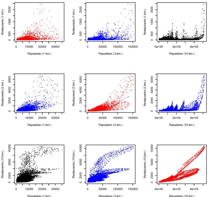
4. Type of amenities—does the relation differ between type of amenities? Figure 2: Non-rural population versus amount of restaurants
8
We start with the spatial dimension. Figure (2) shows for one type of amenity, namely restaurants, the relation between the amount of establishments and population on various spatial scales. The nine subfigures indicate all possible combinations of the radii of 1, 3 and 10 kilometer.5 The horizontal axis denotes the population and the vertical axis the amount of restaurants. Thus, the upper-left corner shows the number of establishments and the
5 To avoid too many missing values or zeros, only the urban grid cells are shown, where we define urban grid cells as grid cells that contain more than 500 households.
9
size of the population within a kilometer radius and the more we read to the right and to the bottom the larger the radius.
Obviously, the choice of the spatial dimension is of crucial importance for the empirical relation and the corresponding specification. For example, the relation between the amount of restaurants and the size of the population is within a one kilometer radius (upper-left corner) far less straightforward than within a 10 kilometer radius (lower-right corner). The location of large amounts of amenities, in this case restaurants, does not necessarily directly imply the location of a large population size. However, if we increase the scale, the relation between amenities and population becomes obviously clearer.6 For the question to
6 Part of this clearer relation is partly explained by the large correlation between observations for larger radii—they simply overlap each other.
10
what extent larger market areas are related with more amenities, it thus seems more natural to answer this question by looking at market areas with larger radii.
Figure (3) shows again the relation between population and amount of restaurants, but only for the four largest cities in the Netherlands (Amsterdam, Rotterdam, The Hague and Utrecht). Clearly, a similar picture emerges as in Figure (2), although the empirical relation is now even more pronounced. This provides empirical evidence (and results with other types of amenities support this) that the relation is city-specific. Thus, the relation between population and amount of amenity differs per municipality. Namely, each almost straight line in the bottom-right subfigure in Figure (3) corresponds with one particular municipality, just as the peaks in the two subfigures above and the two subfigures to the left.
11
This stylized fact entails that the fundamental market area characteristics vary between municipalities. In this case specifically, the municipality of Amsterdam stands out because the relation between population and amount of restaurants is much stronger than for the other three (e.g., the topline in the bottom-right figure denotes the municipality of Amsterdam).This might be caused by the large amount of tourists visiting Amsterdam, but at the same time questions whether results for one municipality can straighforward be transferred to other municipalities.
Note as well, that the nature of this relation is determined by the slope of the line depicted in the last subfigure in Figure (3) and not so much by the size of population or amenities. Thus smaller but equally touristic municipalities (e.g., close to the beaches) may show a similar behavior between amenities and population as in Amsterdam.
Obviously, it matters whether we look at the amount of amenities or the number of employees. The former might be seen as a measure for external economies of scale, where the latter gives a measure for internal economies of scale. Therefore, Figure (4) shows the relation between non-urban population and the number of employees in restaurants. The similarities with (2) are remarkable. The larger the radius of market areas, the more distinguishable the relation between population and number of employees.
The type of amenity is the last dimension we look at. Obviously, the relation between population and amenities may differ per type of amenity. As Section 2 already indicated, the size of market areas depend heavily on the production structure and internal economies of scale. Figure (5) shows for example the relation between population and the number of supermarkets in non-rural areas. Although we see similar patterns as in (2), there are significant differences as well. Most notably, differences between municipalities seem smaller than for restaurants. A possible explanation might be that external economies of scale are less important for supermarkets than for restaurants.
4 Implementation & Results
The previous section showed that the most suitable spatial scale to model market areas with our data is that of market areas with a radius of 10 kilometer. However, Section 3 shows as well that this relation might differ between municipalities, types of amenities and between the amount of employees and the amount of establishments. The next subsection presents an econometric model able to deal with those characteristics, whereas the subsequent subsection offers the results.
4.1 Econometric model
Given the nonlinear structure from Section 2 the most simple model for the relation between population and amenities seems to be 𝐷 = 𝛼𝑃𝛽, where D denotes the market demand for a certain amenity and P the population. In a perhaps too simple exposition: if β is equal to 1, then there are no scale economies present, if β is smaller than 1 then there are
12
diseconomies ofof scale and if β is larger than 1 then there are economies ofof scale.7 Note that β in this case thus should be interpreted as an elasticity, as displayed by the related formula,
ln(𝐷𝑖𝑎) = 𝛼 + 𝛽 ln(𝑃𝑖𝑎) + 𝜖𝑖𝑎, (3) where i denotes gridcell i and a amenity type a, and ε an independent and identically distributed error term, to account for ideosyncratic effects . Because of its linear structure, model (3) can be estimated by ordinary least squares (OLS).
One potential problem with specification (3) is that of unobserved heterogeneity.8 Namely, both population and the demand for amenities might be caused by other, unobserved, factors, such as sector structure and accessibility. To control for this, we introduce municipality specific fixed effects as follows:
ln�𝐷𝑖𝑗𝑎� = 𝛼𝑗+ 𝛽 ln�𝑃𝑖𝑗𝑎� + 𝜖𝑖𝑗𝑎, (4)
where the subscript j now denotes municipality j.
Finally, as Figures (2)—(5) suggest, the relation between population and market demand might differ fundamentally between cities, and a further extension of the proposed model (4) is needed. Therefore, to look at the relation between population and amenities and controlling for city specific slope and level effects we use the following multilevel model:
ln�𝐷𝑖𝑗𝑎� = 𝛼00+ 𝛽00ln�𝑃𝑖𝑗𝑎� + 𝛼1𝑗+ 𝛽1𝑗ln�𝑃𝑖𝑗𝑎� + 𝜖𝑖𝑗𝑎, (5)
where both level and slope parameters α and β are now explicitly extended with a municipality specific random coefficient for both constant and the slope parameter, respectively 𝛼1𝑗 and 𝛽1𝑗 as an addition to their ‘deterministic’ counterparts 𝛼00 and 𝛽00. These latter parameters are considered municipality independent and the elasticity parameter 𝛽00 is treated here as the parameter under investigation, and is directly comparable with the β in equation (4) (see Table 2 in the next section).9
7 Those scale economies now say something about the market area and not so much about the
internal production structure of the firm. It is namely very likely that if β<1, then a firm is better
able to serve a larger market with less resources, which signifies economies to scale at the firm level.
8 Another potential problem could be simultaneity bias. Namely, here it is assumed that population caused market demand, while it might as well be vice versa: market demand causes population growth. Given the rather restrictive Dutch spatial planning policies, this seems however an assumption that is justifiable (see, inter alia, Vermeulen and Rouwendal 2007, de Graaff 2008 et al., Vermeulen and van Ommeren 2009 and de Graaff 2012).
9 Theoretically, specification (5) is superior to specification (4) but relies on more rigid assumptions about the relation between the parameters and the error term. We therefore give both the fixed effects and the multilevel model results.
13
4.2 Results
Table (2) shows the results for models (3)—(5) for various types of amenities (a) and for the relation between employment and population for our whole sample.10
Table 2: Estimated elasticities between population and employment for various specifications (N = 134,841):
Employment in: OLS Fixed effects Multilevel
Cafes
0.88 0.90 1.03Clothes stores
1.25 1.56 1.49Restaurants
0.98 0.91 1.08Supermarkets
1.03 1.15 1.10Shoe stores
1.23 1.56 1.52Libraries
1.09 1.24 1.22Fire brigade
1.37 1.47 1.74Hospitals
1.60 2.17 2.59theaters
1.26 1.72 2.08Note: All parameters are statistically significant at the 0.1% level.
First of all, the type of model matters for the height of the elasticity. Controlling for unobserved heterogeneity or municipality specific parameters seems to increase the values for most various elasticities. Indeed, if population grows then employment in amenities seems to grow relatively even more (except perhaps for cafe’s and restaurants). Note that the more public types of amenities (e.g., hospitals and fire brigades) exhibit the largest elasticities together with theaters. Table A1 in the Appendix gives an overview of the fixed effect results for all spatial levels for only the non-rural areas.
To display the municipality specific slope parameters, we estimate model (4) as well with municipality specific slope parameters and depict them in Figure (6).
As this Figure clearly shows, there are considerable differences between the amount of employees and population between municipalities (this is even more pronounced for the relation between the amount of restaurants and population). What we see is that especially tourist destinations (e.g., Amsterdam and the Wadden islands) show high elasticities. This relationship is directly related with the amount of national and international visitors these areas receive.
14
Figure 6: Relation between number of employees and population
Table 3: Estimated elasticities between population and number of establishments for various specifications (N = 134,841):
Establishments: OLS Fixed effects Multilevel
Cafes
0.82 0.87 1.01Clothes stores
1.08 1.31 1.29Restaurants
0.87 0.84 1.02Supermarkets
0.83 0.86 0.98Shoe stores
1.05 1.22 1.29Libraries
0.54 0.54 0.63Fire brigade
0.41 0.45 0.49Hospitals
0.80 1.00 1.12theaters
0.60 0.73 0.70Note: All parameters are statistically significant at the 0.1% level.
Table (3) shows the results for models (3)—(5) for various types of amenities (a) and for the relation between number of establishments and population for our whole sample. It is striking that, compared with Table (2), all elasticities decrease significantly in size and become either lower than 1 or statistically equal to 1. We only observe robust economies ofscale in the amount of shoe stores and clothing stores. Thus, if the number of population
15
increases, the number of these type of amenities increases even more. This might point to consumer externalities considering those kind of amenities.
For the public amenities, the differences are however remarkable. If the population grows, the amount of employees within these kinds of amenities grows but the number of facilities decreases. So, within larger urban areas you do not find more libraries, fire brigades and hospitals per capita, but you find instead larger establishments, which thus points to (perceived) internal economies ofscale. For cafes, restaurants and supermarkets it seems that these amenities operate under constant returns to scale.
5 Discussion
Our results show that internal economies of scale seem to dominate external economies of scale. We have to be careful to draw such an explicit conclusion. First of all, the lack of external economies of scale in Table (3) for the public amenities might also be caused by the Dutch policies of scaling up these amenities and not so much by internal economies of scale within the production structure. For private amenities, which operate in competitive markets, a direct link between the elasticities in Table (3) and economies of scale is more conceivable.
Moreover, we assume homogeneous workers. If more urbanized areas receive higher skilled workers, then amenities need less workers to be equally productive. This additional sorting effect might bias the results found in (2) and (3) and especially the distinction between urban and rural areas. Apart from this particular sorting effects, there might be other sorting effects that, e.g., describe how population seeks to live in municipalities that best fit their preferences (a ‘voting by the feet’ mechanism).
Our results do have two direct policy implications. Firstly, if the interpretation is correct that some municipalities have more—and thus a larger variety of—amenities because of more visitors, then municipalities should not focus on increasing population size, but instead on increasing the number of visitors. This, however, induces a chicken and egg problem. Municipalities become more attractive because of a larger amount of amenities, but those amenities can only be sustained in the first place by having a large amount of visitors. Secondly, we show that when a municipality’s population grows, the size of most amenities grows but not its number. This is beneficial in terms of employment but not in terms of consumer externalities. Except for shoe and clothes stores, a positive feedback mechanism in the number of amenities when population grows is not very likely. Thus, one should be reluctant in social cost-benefit analyses to consider bandwagon effects of local population increase as potential benefits.
6 Conclusions
This paper focused on the empirical relation between amenities and population in the Netherlands, and especially scrutinized two aspects. First, we investigated to what extent size and number of amenities change if population changes and whether there are
16
structural differences between types of amenities and across municipalities. Secondly, we looked at the distinction between amenities measured by the number of employees and the number of establishments.
Our main conclusions can be summarized as follows. First of all, it seems that internal economies of scale dominate the external economies of scale (at least for the type of amenities we research). This seems especially prevalent for public facilities. This might also point to the conclusion that urban externalities manifest themselves mostly at the production side and not so much at the consumption side.
Secondly, we find that the structural relation between population and amenities becomes clearer at larger spatial aggregation levels. Too small a spatial scale—without taking into account travel or transportation distances—might bias the resulting inference. Namely, market areas of many amenities seem to have a larger radius than one kilometer. In our data, market areas with 10 kilometer radius seems to be most appropriate spatial scale for our analysis.
Moreover, there seems to be structural differences between both amenities and municipalities. Not all amenities seem to exhibit similar scale economies—which, obviously, depends on their internal production structure—and the elasticity between market demand and population might as well differ over municipalities. The latter is probably partly due to the large amount of both national and international visitors that some municipalities (e.g., Amsterdam, Delft, and Haarlem) receive.
Finally, we find consistent internal and external economies of scale for clothing and shoe stores. On the other hand, we do not find them for theaters, restaurants and cafes—which are traditional entertainment sectors in the Netherlands. So, where for shopping we find some evidence for consumer externalities, we do not find them for other ‘leisure’ activities.
Acknowledgements
This paper is written in the context of the PBL-CPB project ‘Plannen voor de stad’ and serves as a technical background paper for the corresponding report’s Chapter 5. We gratefully acknowledge the valuable contributions, comments and suggestions by Marnix Breedijk, Rietveld, Jan Rouwendal, Henri de Groot, Gusta Renes, Gerbert Romijn, Frank van Oort.
References
Ades, A. F. and E. L. Glaeser (1995). “Trade and Circuses - Explaining Urban Giants”.
Quarterly Journal of Economics 110.1, pp. 195–227.
Baum-Snow, N and R Pavan (2012). “Understanding the City Size Wage Gap”. Review of
Economic Studies 79.1, pp. 88–127.
Beckman, M. J. (1958). “City Hierarchies and the distribution of city size”. Economic
Development and Cultural Change 6, pp. 243–248.
Berry, B. J. L. and W. L. Garrison (1958). “A Note on Central Place Theory and the Range of A Good”. Economic Geography 34.4, pp. 304–311.
Christaller, W (1966). Central Places in Southern Germany. trans. C.W. Baskin, Englewood: Prentice Hall (cit. on p. 4).
Combes, P. P. (2000). “Economic structure and local growth: France, 1984-1993”. Journal
17
Combes, P. P., G Duranton, and L Gobillon (2008). “Spatial wage disparities: Sorting matters!” Journal of Urban Economics 63.2, pp. 723–742.
— (2011). “the identification of agglomeration economies”. Journal of Economic Geography 11, pp. 253–266.
Duranton, G (2003). “Economics of agglomeration: Cities, industrial location and regional growth”. Urban Studies 40.4, pp. 854–856
Duranton, G and H. G. Overman (2005). “Testing for localization using micro-geographic data”. Review of Economic Studies 72, pp. 1077–1106.
Fujita, M, P Krugman, and A. J. Venables (1999). The Spatial Economy: Cities, Regions, and
Economic Trade. Cambridge: MIT Press.
Fujita, M and J. F. Thisse (2002). Economics of Agglomeration: Cities, Industrial Location
and Regional Growth. Cambridge: Cambridge University Press.
Glaeser, E. L. and J. D. Gottlieb (2006). “Urban resurgence and the consumer city”. Urban
Studies 43.8, pp. 1275–1299.
Glaeser, E. L., J Gyourko, and R Saks (2006). “Urban Growth and Housing Supply”. Journal
of Economic Geography 6.1, pp. 71–89.
Glaeser, E. L., J Kolko, and A Saiz (2001). “The consumer city”. Journal of Economic
Geography 1.1, pp. 27–50.
Graaff, T de, F van Oort, and S Boschman (2008). Woon-werkdynamiek in Nederlandse
gemeenten. Rotterdam/Den Haag: NAi Uitgevers/Ruimtelijk Planbureau.
Graaff, T de, F. G. van Oort, and R. Florax (2012). “Regional Population-Employment Dynamics Across Different Sectors of the Economy”. Journal of Regional Science 52.1, pp. 60–84.
Groot, H de et al. (2010). “City and countryside”. The Hague, Netherland Bureau for Economic Policy Analysis (in Dutch).
Henderson, J. V. (1982). “Evaluating consumer amenities and interregional welfare differences”. Journal of Urban Economics 11, pp. 32–59.
Henderson, J. W., T. M. Kelly, and B. A. Taylor (2000). “The impact of agglomeration economies on estimated demand thresholds: An extension of Wensley and Stabler”.
Journal of Regional Science 40.4, pp. 719–733.
Krugman, P (1991). “Increasing Returns and Economic-Geography”. Journal of Political
Economy 99.3, pp. 483–499.
Lösch, A (1954). The economics of location. New Haven: Yale University Press.
Melo, P. C., D. J. Graham, and R. B. Noland (2010). “A meta-analysis of estimates of urban agglomeration economies”. Regional Science and Urban Economics 39.3, pp. 332– 342.
Mushinski, D and S Weiler (2002). “A note on the geographic interdependencies of retail market areas”. Journal of Regional Science 42.1, pp. 75–86.
O’Sullivan, A (2003). Urban Economics. New York: McGraw-Hill.
Puga, D (2010). “The Magnitude and Causes of Agglomeration Economies*”. Journal of
Regional Science 50.1, pp. 203–219.
Roback, J (1982). “Wages, rents and the quality of life”. Journal of Political Economy 90.6, pp. 1257–1278.
Shonkwiler, J. S. and T. R. Harris (1996). “Rural retail business thresholds and interdependencies”. Journal of Regional Science 36.4, pp. 617–630.
Vermeulen, W and J van Ommeren (2009). “Does land use planning shape regional economies? A simultaneous analysis of housing supply, internal migration and local employment growth in the Netherlands”. Journal of Housing Economics 18.4, pp. 294–310.
Vermeulen, W and J Rouwendal (2007). “Housing Supply and Land Use Regulation in the Netherlands”. Tinbergen Institute Discussion Paper, TI 2007-058/3, Amsterdam. Wensley, M. R. D. and J. C. Stabler (1998). “Demand-threshold estimation for business
18
A Appendix
Table A.1: Estimated elasticities of employment size and population for various levels of scale with fixed effects (all urban areas: N=14,343)a
Spatial scale(1 km.)
Employment in: Population (1 km.) Population (3 km.) Population (10 km.)
Cafes 0.83 0.22 −0.14 Clothing stores 1.39 0.68 −0.68 Restaurants 0.70 0.40 −0.09 Supermarkets 1.49 0.02 −0.34 Shoestores 0.40 1.35 −0.86 Libraries 0.44 0.62 −0.20 Fire-brigades −0.33 1.06 0.07 Hospitals −0.82 1.77 0.14 theaters 0.20 1.62 0.78 Spatial scale (3 km.)
Employment in: Population (1 km.) Population (3 km.) Population (10 km.)
Cafes −0.01 1.29 −0.20 Clothing stores −0.11 2.26 −0.64 Restaurants −0.02 1.28 −0.06 Supermarkets 0.04 1.50 −0.41 Shoestores −0.08 2.05 −0.48 Libraries 0.05 1.31 −0.03 Fire-brigades −0.20 1.29 0.18 Hospitals −0.25 2.03 0.06 theaters −0.15 1.97 1.40 Spatial scale (10 km.)
Employment in: Population (1 km.) Population (3 km.) Population (10 km.)
Cafes 0.00 0.00 1.10 Clothing stores 0.00 0.02 1.53 Restaurants 0.01 −0.01 1.12 Supermarkets 0.00 0.02 1.07 Shoestores 0.00 0.01 1.58 Libraries 0.02 −0.01 1.29 Fire-brigades 0.00 −0.08 1.65 Hospitals 0.00 −0.19 2.61 theaters 0.02 −0.11 2.26
a Given the large number of observations, almost all variables are significant at a 5% level. The rows
indicate the various endogenous variables and the columns the various exogenous variables. Thus, The regression reads in this case from left to right.
19
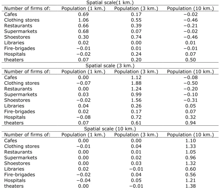
Table A.2: Estimated elasticities of number of firms and population for various levels of scale with fixed effects (all urban areas: N=14.343)a
Spatial scale(1 km.)
Number of firms of: Population (1 km.) Population (3 km.) Population (10 km.)
Cafes 0.69 0.17 −0.02 Clothing stores 1.06 0.55 −0.46 Restaurants 0.66 0.39 −0.21 Supermarkets 0.68 0.07 −0.02 Shoestores 0.30 0.74 −0.46 Libraries 0.02 0.00 0.01 Fire-brigades −0.01 0.01 −0.01 Hospitals −0.02 0.24 0.07 theaters 0.07 0.20 0.50 Spatial scale (3 km.)
Number of firms of: Population (1 km.) Population (3 km.) Population (10 km.)
Cafes 0.00 1.12 −0.08 Clothing stores −0.07 1.88 −0.50 Restaurants 0.00 1.24 −0.20 Supermarkets 0.03 0.99 −0.10 Shoestores −0.02 1.56 −0.31 Libraries 0.04 0.26 0.05 Fire-brigades 0.02 0.17 0.07 Hospitals −0.08 0.72 0.32 theaters 0.07 0.61 0.94 Spatial scale (10 km.)
Number of firms of: Population (1 km.) Population (3 km.) Population (10 km.)
Cafes 0.00 0.00 1.10 Clothing stores −0.01 0.04 1.33 Restaurants 0.00 0.01 1.05 Supermarkets 0.00 0.02 0.96 Shoestores 0.00 0.03 1.32 Libraries 0.02 −0.01 0.60 Fire-brigades −0.02 0.04 0.56 Hospitals −0.04 0.05 1.21 theaters 0.00 −0.01 1.38
a Given the large number of observations, almost all variables are significant at a 5% level. The rows
indicate the various endogenous variables and the columns the various exogenous variables. Thus, The regression reads in this case from left to right.