TAPWAT: Definition structure and applications for modelling drinking water treatment | RIVM

Hele tekst

(1)research for man and environment. RIJKSINSTITUUT VOOR VOLKSGEZONDHEID EN MILIEU NATIONAL INSTITUTE OF PUBLIC HEALTH AND THE ENVIRONMENT. RIVM rapport 734301 019 TAPWAT: Definition, structure and applications for modelling drinking-water treatment. J.F.M Versteegh, F.W. van Gaalen, L.C.1), Rietveld E.G. Evers, T.A. Aldenberg and P. Cleij March 2001. 1) Technische Universiteit Delft Dit onderzoek werd verricht in opdracht en ten laste van DGM/BWL, in het kader van project 734301, Normstelling en handhaving drinkwater, mijlpaal TAPWAT rapportage. RIVM, Postbus 1, 3720 BA Bilthoven, telefoon: 030 - 274 91 11; fax: 030 - 274 29 71.

(2) pag. 2 van 65. RIVM rapport 734301 019. Abstract The ‘Tool for the Analysis of the Production of drinking WATer’ (TAPWAT) model has been developed for describing drinking-water quality in integral studies in the context of the Environmental Policy Assessment Function of the RIVM. The model consists of modules that represent individual steps in a treatment process, so that different treatment processes can be constructed. The treatment steps included in TAPWAT are used mainly in systems for the treatment of surface water. The current version of TAPWAT described in this report consists of modules based on removal percentages and on process or semi-empirical modelling. Stochastic modelling using beta-distribution has been worked out for two treatment steps and seems to be a promising technique; however, the availability of data for individual treatment steps is a disadvantage. In general, this combination works out fairly well in the model structure developed for TAPWAT. The model must be able to cover, at least for pathogens, the pathway from water source to infection risk for the public. The parts of the puzzle are present, but the puzzle still has to be laid. The model is as yet only suitable for operation by experts. A plan of action is recommended in which the existing and missing modules, compounds and micro-organisms of interest will be prioritised and the necessary validation of the model described. This plan of action should be implemented to improve the current TAPWAT version and make it suitable for assess public health risks..

(3) RIVM rapport 734301 019. pag. 3 van 65. Preface This report describes the main features of the model, TAPWAT, constructed at the RIVM in cooperation with the Delft University of Technology. The project was set up mainly to construct a mathematical model that, could calculate, the removal of micro-organisms and chemicals, on the one hand and the formation of by-products, on the other, on a global spatial scale during the drinking-water production process. The current version of the model described in this report aims at the treatment of surface water and, in particular, the removal of micro-organisms and the formation of disinfection byproducts. Our thank goes out to the drinking-water supply companies for providing the data used in this project. We also thank our colleagues in Bilthoven and Delft for their useful comments and support during the course of the project..

(4) pag. 4 van 65. RIVM rapport 734301 019. Contents. 4. Summary. 6. Samenvatting. 8. 1. Introduction. 11. 2. Definition of the model TAPWAT. 13. 3. 4. 5. 2.1. Goals of the model. 13. 2.2. Parameters and treatment steps. 13. 2.3 Approach of modelling 2.3.1 Percentage removal 2.3.2 Process or semi-empirical modelling 2.3.3 Stochastic modelling. 13 13 14 14. 2.4. 14. Applications of TAPWAT. The concept of the model TAPWAT. 15. 3.1. Introduction. 15. 3.2. Basic principles from the definition study. 15. 3.3 Input and output of TAPWAT 3.3.1 Input data 3.3.2 Specification of the input files 3.3.3 Output data 3.3.4 Specification of the output files. 16 16 17 17 18. 3.4 Input and output of a treatment module 3.4.1 Input of a treatment module 3.4.2 Output of a treatment module. 18 18 18. 3.5. Monte Carlo analysis in TAPWAT. 18. 3.6. Steps to be performed by the model. 19. Determination of removal percentages. 21. 4.1. Introduction. 21. 4.2. Removal percentages based on data from databases and literature. 21. 4.3. Removal percentages based on data of drinking-water production plants. 21. 4.4. Determination of removal percentages based on results of treatment plants. 23. 4.5. General conclusions from the data analysis. 24. Process or semi-empirical modelling 5.1. Introduction. 5.2 Chlorination 5.2.1 Modelling the HOCl/OCl--equilibrium 5.2.2 Giardia 5.2.3 Cryptosporidium 5.2.4 Enterovirus 5.2.5 Trichloromethane. 29 29 29 29 30 30 31 31.

(5) RIVM rapport 734301 019. 5.2.6 5.2.7 5.2.8. 6. 7. Bromodichloromethane Trichloroacetic acid Verification of formation of trichloromethane by chlorination. 32 33 33. 5.3 Ozonation 5.3.1 Giardia 5.3.2 Cryptosporidium 5.3.3 Enterovirus 5.3.4 Bromate. 35 35 35 36 37. 5.4. 38. Conclusions. Stochastic modelling of the removal of natural organic compounds in drinking-water processes. 39. 6.1. Introduction. 39. 6.2. Removal of organic compounds in conventional drinking-water treatment processes. 39. 6.3. Beta-distribution. 41. 6.4. Distribution of removal of Total Organic Carbon by floc formation and removal. 42. 6.5. Distribution of removal of Total Organic Carbon by activated carbon. 43. 6.6. Conclusions. 44. Validations and applications of TAPWAT 7.1. 8. pag. 5 van 65. Introduction. 47 47. 7.2 Validation of TAPWAT based on company data 7.2.1 Basic assumptions 7.2.2 Example of the results 7.2.3 Conclusions. 47 47 47 49. 7.3 Balancing the risks of micro-organisms and disinfection by-products as an application 7.3.1 Basic assumptions 7.3.2 Results. 50 50 51. 7.4 Application of TAPWAT for the National Environmental Outlook 7.4.1 Basic assumptions 7.4.2 Example of the results 7.4.3 Conclusions. 52 52 53 55. 7.5. Example of statistical analysis. 56. Conclusions and recommendations. 57. 8.1. Conclusions. 57. 8.2. Recommendations. 58. References. 59. Annex 1. Mailinglist. 63. Annex 2. References (table 4.2). 64.

(6) pag. 6 van 65. RIVM rapport 734301 019. Summary The model, TAPWAT (Tool for the Analysis of the Production of drinking WATer), has been developed for describing drinking-water quality in integral studies in the context of the Environmental Policy Assessment Function of the RIVM. TAPWAT consists of modules that represent individual steps in a treatment process, so that different treatment processes can be constructed. The steps included in TAPWAT are used mainly in systems for the treatment of surface water. The current version of TAPWAT, described in this report, consists of modules based on removal percentages and on process or semi-empirical modelling. In general, this combination works out fairly well in the model structure developed for TAPWAT. Modules based on removal percentages Removal percentages and ranges are derived from existing database, found in the literature and derived from pilot and full-scale treatment plants. There is a lack of measurement data, especially for the individual treatment steps and target compounds like pathogenic microorganisms and pesticides. About 15% of the ranges are based on detailed data from watersupply companies. Of the data on five micro-organisms of interest for public health or an indicator, only data for spores of sulphite-reducing clostridia (SSRC) are available. The removal of pathogenic micro-organisms is based on numbers of logarithmic reduction derived from field studies or experiments at pilot treatment plants. For the organic micro-pollutants and heavy metals (six compounds), data availability is very limited and even absent for two compounds. Data availability is reasonable for disinfection by-products. Validation is done for two parameters in an example of a treatment process, it worked out well for the data-rich parameter. The uncertainty of the percentage ranges is the lowest when the ranges are derived from full-scale treatment plants. Modules based on process or semi-empirical modelling In TAPWAT the chlorination and ozonation modules are incorporated for the prediction of disinfection by-products and the removal of micro-organisms. These modules are based on empirically based equations. Examples for the prediction of the formation of disinfection byproducts give reasonable results. Stochastic modelling is done for two treatment steps (floc formation and removal, and activated carbon filtration). Stochastic modelling using betadistribution is a promising technique; however, the lack of available data from individual treatment steps is a disadvantage. Only indicator parameters or parameters which are easy and cheap to measure are suitable. Model calibration and validation Data from full-scale treatment plants should be used as much as possible for model calibration and validation, both for percentages and the process modules of TAPWAT. The availability of data is limited, especially for individual treatment steps and non-system parameters like pesticides. Pilot-scale and laboratory data will have to fill the (many) gaps. Only a few validations are done with TAPWAT. For the most interesting parameters like pesticides and pathogens, either data is lacking or there are too many measurements below detection limit. Indicators should be used for the pathogens; however, there are still a lot of.

(7) RIVM rapport 734301 019. pag. 7 van 65. ‘below-detection-limit’ data. The subject on how to calculate the removal of micro-organisms has been described in a separate report (Evers and Groennou, 1999). General expressions for the estimation of value µ (average in the beta-distribution) should be formulated for use in stochastic modelling. This value is specific for each treatment plant but can be made more general to improve of the usefulness of TAPWAT, for example, by analysing measurement data of more plants in the same way. The modules in TAPWAT are based on an average performance of treatment steps; this can differ from the performance of a treatment step in a particular treatment system. Caution will be needed when applying the model to specific cases. The main goal of TAPWAT is to use the model in global-scale studies for the Netherlands. Recommendations TAPWAT is a model suitable for application on a global scale in treatment plants using, surface water as the raw water source. The model described is not yet completed. The modules based on removal percentages should be updated regularly, and those based on process or semi-empirical modelling have to be validated for more systems, so that the uncertainty of the results can be described on a higher level. New model studies for soil passage have been recently published (Schijven, 2001), the results of which should be incorporated in TAPWAT. Considering that the UV-disinfection technique has now become more important for the removal of pathogens like viruses and protozoa, a module for UV should be incorporated in TAPWAT. Membrane technology is used more and more for piped water production like drinking water and household water. Information available from pilot and full-scale plants should be used to improve the existing modules. The model must be able, at least for pathogens, to cover the pathway from water source to infection risk for the public. The parts of the puzzle are present but the puzzle still has to be laid. The model is as yet only operable for experts. To make it suitable for non-experts an update of the current version with input screens etc. has to be made. This work should be put out to a contractor. A plan of action is recommended in which the existing and missing modules, compounds and micro-organisms of interest are prioritised and the necessary validation of the model carried out. To both improve the current TAPWAT version and make it also suitable for public health risk assessment the plan of action should be carried out by experts and model updates eventually put out to a contractor..

(8) pag. 8 van 65. RIVM rapport 734301 019. Samenvatting Het model TAPWAT (Tool for the Analysis of the Production of drinking WATer), is ontwikkeld om de drinkwaterkwaliteit te beschrijven voor integrale studies in het kader van de planbureaufunctie van het RIVM. Het model bestaat uit modules die de individuele zuiveringsstappen van het drinkwaterzuiveringsproces vertegenwoordigen. De zuiveringsstappen in TAPWAT worden voornamelijk gebruikt in systemen voor de behandeling van oppervlaktewater. De huidige versie van TAPWAT, zoals in dit rapport beschreven, bestaat uit modules gebaseerd op verwijderingspercentages en modules gebaseerd op proces of semi-empirische modelering. Modules gebaseerd op verwijderingspercentages Verwijderingspercentages and ranges daarvan zijn verkregen vanuit bestaande databestanden, uit de literatuur, vanuit proefinstallaties en van volledig in bedrijf zijnde zuiveringsstations. Er is een gebrek aan meetgegevens vooral voor wat betreft de individuele zuiveringsstappen en voor de belangrijke parameters zoals pathogene micro-organismen en bestrijdingsmiddelen. Ongeveer 15% van de ranges zijn gebaseerd op gedetailleerde gegevens van waterbedrijven. Van de vijf micro-organismen van belang voor de volksgezondheid of als indicator-organisme hiervoor, zijn er uitsluitend gegevens voor sporen van sulfiet reducerende clostridia beschikbaar. De verwijdering van pathogene micro-organismen is gebaseerd op aantallen logaritmische eenheden reductie verkregen uit veldstudies of uit experimenten met proefinstallaties. De beschikbaarheid van gegevens voor de organische micro-verontreinigingen en zware metalen (zes stoffen) is erg beperkt en de gegevens voor twee stoffen zijn zelfs afwezig. De beschikbaarheid van gegevens is redelijk voor desinfectiebijproducten. Validatie is uitgevoerd voor één casus en twee parameters, en werkt goed voor een parameter waarvoor veel gegevens beschikbaar zijn. De onzekerheid in het percentage ranges is het laagst wanneer de ranges afkomstig zijn van volledig in bedrijf zijnde zuiveringsstations. Modules gebaseerd op proces of semi-empirische modelering In TAPWAT zijn de modules chloring en ozonisatie aanwezig om de verwijdering van microorganismen te beschrijven en de vorming van desinfectiebijproducten te voorspellen. Deze modules zijn gebaseerd op empirisch verkregen formules. Voorbeelden van de voorspelling over de vorming van desinfectiebijproducten geven redelijke resultaten. Stochastische modelering is uitgevoerd voor twee zuiveringsstappen (vlokvorming en vlokverwijdering en voor actieve koolfiltratie). Stochastische modelering met behulp van de beta-verdeling is een veel belovende methodiek hoewel de geringe beschikbaarheid van data voor de individuele zuiveringsstappen een nadeel is. Model calibratie en validatie Gegevens afkomstig van zuiveringsstations zullen zoveel mogelijk gebruikt dienen te worden voor modelcalibratie en modelvalidatie, zowel voor percentage als voor procesmodules in TAPWAT. De beschikbaarheid van gegevens is beperkt vooral voor individuele zuiveringsstappen en niet-systeemparameters zoals bestrijdingsmiddelen. Proefinstallaties en laboratoriumgegevens zullen de vele gaten in het databestand moeten vullen. Er is een beperkt aantal validaties uitgevoerd met het model TAPWAT. Voor de meest interessante parameters als bestrijdingsmiddelen en pathogenen is er een tekort aan gegevens.

(9) RIVM rapport 734301 019. pag. 9 van 65. of zijn er teveel metingen beneden het detectieniveau. Voor de pathogenen zullen indicatoren gebruikt moeten worden maar ook dan zijn er veel meetresultaten beneden de detectiegrens. Het onderwerp hoe de verwijdering van micro-organismen te berekenen is beschreven in een separaat rapport (Evers en Groennou, 1999). Als stochastische modelering gebruikt wordt zullen algemene uitdrukkingen voor de schatting van de waarde µ (gemiddelde in de beta-verdeling) dienen te worden vastgesteld. Deze waarde is specifiek voor elk zuiveringsstation maar kan meer algemeen worden gemaakt in het belang van de bruikbaarheid van TAPWAT. Een mogelijkheid om dit uit te voeren is om meetgegevens van andere stations op dezelfde manier te analyseren. De modules in TAPWAT zijn gebaseerd op de gemiddelde prestatie van zuiveringsstappen; dit kan afwijken van de prestatie van een zuiveringsstap in een individueel zuiveringsproces. Voorzichtigheid is geboden met het gebruik van het model voor specifieke systemen. Het belangrijkste doel van TAPWAT is om het model te gebruiken voor globale studies binnen Nederland, zogenaamd landsdekkend. Aanbevelingen TAPWAT is een model dat gebruikt kan worden op globale schaal voor zuiveringsstations die oppervlaktewater als bron gebruiken. Het in dit rapport beschreven model is nog niet compleet. De modules gebaseerd op verwijderingsspercentages zullen regelmatig geüpdate moeten worden, de modules gebaseerd op proces of semi-empirische modelering dienen voor meer systemen gevalideerd te worden zodat de onzekerheid in de resultaten beter beschreven kan worden. Recent zijn nieuwe studies gepubliceerd (Schijven, 2001) voor bodempassage, deze zullen in TAPWAT geïncorporeerd worden. De techniek UV-desinfectie wordt steeds belangrijker voor de verwijdering van pathogenen als virussen en protozoa. Een module hiervoor zal in TAPWAT geïncorporeerd dienen te worden. Membraantechnologie wordt meer en meer gebruikt voor de productie van leidingwater als drink- en/of huishoudwater. Beschikbare informatie van proefprojecten of in bedrijf zijnde zuiveringsprocessen kunnen gebruikt worden om de bestaande modules te verbeteren. Het model moet in staat zijn om het gehele pad te beschrijven van bron tot en met infectierisico voor de bevolking (tenminste voor pathogenen). De delen van de puzzel zijn beschikbar maar de puzzel dient nog wel in elkaar gezet te worden. Het model is nu alleen geschikt voor ‘experts’. Om het voor een breder publiek geschikt te maken zal de huidige versie uitgebreid moeten worden met bijvoorbeeld invoerschermen. Aanbevolen wordt dit onderdeel uit te besteden. Aanbevolen wordt een plan van aanpak te maken waarin de bestaande en de nog missende modules, stoffen en micro-organismen worden aangegeven. De implementatie hiervan in TAPWAT dient vervolgens geprioriteerd te worden in de tijd evenals de noodzakelijke validatie van het model. De verbetering van de huidige versie van TAPWAT en de voorgestelde slag om het model geschikt te maken voor risicoanalyse ten behoeve van de volksgezondheid zal volgens het plan van aanpak uitgevoerd moeten worden door deskundigen of desnoods worden uitbesteed..

(10) pag. 10 van 65. RIVM rapport 734301 019.

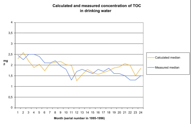
(11) RIVM rapport 734301 019. pag. 11 van 65. 1 Introduction The main goal of the department of environmental research of the National Institute of Public Health and the Environment (RIVM) is to produce general reports for the Dutch government. The main products are: • State of the environment ‘Milieubalans’ • State of the nature ‘Natuurbalans’ • Environmental outlook ‘Milieuverkenningen’ • Nature outlook ‘Natuurverkenningen’ In these reports subjects are presented for which the activities of the society have a negative effect (pressure) on nature and environment. Some examples of these subjects are the consumption of energy, the production of carbondioxide by the traffic, which are reported at one side. At the other side the quality of water, soil and air is reported in relation with environmental themes as acidification, eutrophication and climate change. In the ‘State of the environment’ the purposes of the government to improve the quality of the environment are confronted with the state of the quality of the environment. For this purpose, indicators are used focussing on the subject drinking water e.g. the quality of the sources for drinking water related to nitrate and pesticides. The quality of the product drinking water is classified as an effect on public health. To be able to produce these reports the whole chain of drinking-water production from source to tap is reviewed. For this purpose mathematical models are constructed for various subjects. In this report one of these models named TAPWAT is presented. TAPWAT means Tool for the Analysis of the Production of drinking WATer. TAPWAT is a tool to predict the purification efficiency of a drinking-water production plant used to purify surface water and/or ground water into drinking water. The input for TAPWAT is the raw water quality for chemicals and micro-organisms. The output is the quality of the drinking water for the parameters, which can be analyzed by the model. For this, the complete purification process was split up in physically separate units. The model can be simple: a module with only a removal percentage for certain parameters or a description of the water treatment process in model formulations in a process module. In chapter 2 the principles of the model are described; in chapter 3 the concept is described and the chapters 4 and 5 the technical modules (percentages and process) are described. Chapter 6 give the main results of the stochastic modelling, chapter 7 gives examples of validation, applications of the model and chapter 8 gives conclusions and recommendations. In a separate report the modules are described in more detail (Rietveld et al., 2001)..


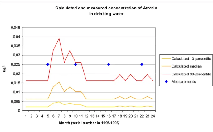
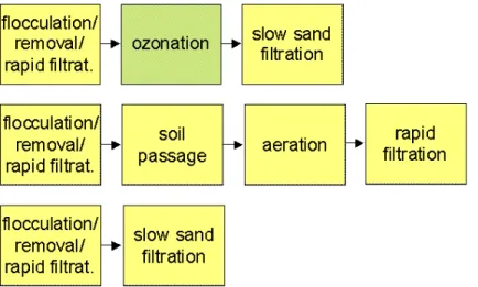
(13) RIVM rapport 734301 019. pag. 13 van 65. 2 Definition of the model TAPWAT In this chapter information is presented about the realisation of the model TAPWAT except the technical information. This information is based on the definition study of TAPWAT (Kragt et al., 1996).. 2.1 Goals of the model The main applications of the model are: • To predict on a global scale, the quality of drinking water (including health risks levels by micro-organisms) given a certain raw water quality. • To advise the Drinking-water Inspectorate by reviewing new or renewed production plants especially concerning public health risks. The model is developed according two pathways: empirical or percentages and process modules. The modules are incorperated in one modelstructure so the modules from both pathways can be used for one application. The model is developed according RIVM standards for information infrastructure and modelling.. 2.2 Parameters and treatment steps In the definition study all available treatment steps at one side and all for drinking water relevant micro-organisms and chemical compounds at the other side were studied. This resulted in a long list with parameters and treatment steps. Review of this list and expert judgement resulted in a matrix with parameters and treatment steps which had the priority to be modelled (Kragt et al., 1996). The following parameters were chosen for different reasons as a representive of the group or the availability of data or expected to be a relevant problem: Micro-organisms: Giardia, Cryptosporidium, enteroviruses and their indicators Pesticides: atrazin, glyfosaat and 1,2-dichloropropane Disinfection byproducts: bromate and trihalomethanes Metals: nickel, cadmium, chromium Process parameters: pH, temperature, DOC, turbidity and bromide. The following treatment steps were chosen because they are a part of surface water treatment and they have the capacity to remove the interesting compounds: Storage reservoir, chlorination, ozonation, floc formation/floc removal, rapid sand filtration, activated carbon filtration, membrane filtration and slow sand filtration.. 2.3 Approach of modelling 2.3.1 Percentage removal Information was collected from literature, reports, data from production plants and sometimes expert judgement to design ranges of percentages for removal micro-organisms and compounds by the selected treatment steps. This process is described in chapter 4. Data from production plants were prefered above pilot plant data or laboratorium experiments. But data of production plants for the chosen compounds and individual treatment steps are scarce..

(14) pag. 14 van 65. RIVM rapport 734301 019. For compounds like metals and pesticides modules based on removal percentages will be good enough for the purpose for which TAPWAT is used. This all results in a number of modules based on ranges of removal percentages which can be used for global sudies. Monte Carlo analysis can be used to find the most probable result when more parameters are used for calculations.. 2.3.2 Process or semi-empirical modelling The design of a process module was done following a sjabloon, a test procedure plan including reporting of the results. In chapter 5 of this report a short description is given for a few modules especially chlorination and ozonation which are used in the current version of the model TAPWAT. More details can be find in internal documents and in Rietveld et al., 2001.. 2.3.3 Stochastic modelling The beta-distribution is used for statistical analyses of data of production plants especially for the removal of TOC and turbidity by flocculation and floc removal and activated carbon filtration. This statistic technique is useful to develope empirical models if enough data of individual parameters from production plants are available.. 2.4 Applications of TAPWAT The model will be used to describe the drinking-water quality in integral studies, examples are given in the last chapter of this report. The connections with other models are still under construction in a separate project..

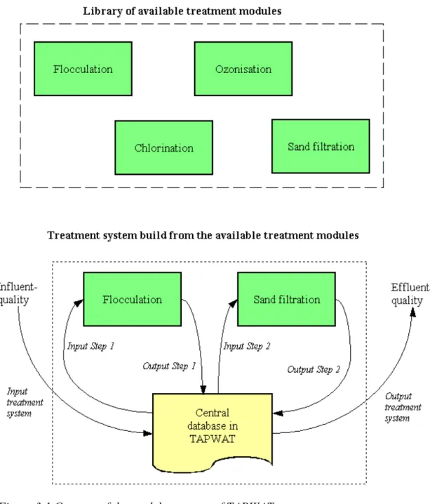
(15) RIVM rapport 734301 019. pag. 15 van 65. 3 The concept of the model TAPWAT 3.1 Introduction In this chapter the principles forming the basis for the realisation of the model TAPWAT will be described. These principles will be based on the definition study of TAPWAT (Kragt et al., 1996), an outline of which is included in the previous chapter. A complete description of the technical concept of TAPWAT can be found in the LWD-report ‘Ontwerp modelstructuur van TAPWAT’ (van Gaalen et al., 1999). A number of aspects mentioned in the definition study (Kragt et al., 1996) serve as starting points for the technical concept of TAPWAT. These aspects will be summarised below.. 3.2 Basic principles from the definition study For the purpose of flexibility the model will consist of modules that represent individual treatment steps in a treatment system. This concept offers the possibility to build different treatment systems by means of a library of modules, as well as allowing replacement of modules by improved ones. The necessary in- and output can differ for every combination of module and substance. To allow for flexible applicability and interchangeability of modules, it is necessary for them to communicate by means of a general interface, with which all the required information can be exchanged. Communication doesn’t take place directly between modules, but by way of a general part of the model that henceforth will be called the model structure. In a central database, that constitutes part of the model structure, the information to be exchanges will be stored (temporarily). The model structure will also have to provide for the possibility of putting together a treatment system on the basis of available treatment modules and for the communication between the model and the user. This concept is schematically shown in Figure 3.1. The model will be built in the MATLAB/Simulink-environment on MS-Windows-PC’s..

(16) pag. 16 van 65. RIVM rapport 734301 019. Figure 3.1 Concept of the model structure of TAPWAT. 3.3 Input and output of TAPWAT In this paragraph the required in- and output of the model will be examined, as well as the form in which it can be entered.. 3.3.1 Input data The input of TAPWAT, i.e. the data to be provided by the user in order to perform a calculation, consists of: • The composition of the treatment system concerned (which treatment modules in what order); • Design- and process parameters of the treatment steps present in the treatment system (design parameters are considered as fixed after building the step; process parameters can be changed after building the step to influence the performance of the process); • Starting conditions of the treatment steps present in the treatment system;.

(17) RIVM rapport 734301 019. • •. pag. 17 van 65. Name and concentration in raw water of the substances or substance groups to be purified (i.e. to be calculated), possibly substance properties also; Name and concentration in raw water of other quality parameters that can influence the amount of purification.. Not all information is needed for every module. The person building a module determines what input is required, on the basis of the kind of modelling to be pursued and the complexity of the processes described. The input needed will be stated in the specifications of a module; in this way a user will know what input the model expects.. 3.3.2 Specification of the input files The following ten input files will be used to provide TAPWAT with the necessary information: • General run data: these determine a number of general aspects of the calculations to be performed, such as the time period to be considered and the number of draws to be performed in the Monte Carlo analysis (see 3.5); • Composition of the treatment system and the substances to be calculated; • Design- and process parameters; • Input concentrations; • Starting conditions; • Substance groups; • Substance properties; • Relation modules – treatment steps; this relation enables every module to use the values of the design/process parameters relating to the step and the treatment station concerned; • Removal percentages of simple empirical modules: name module, name substance, removal percentage. For the purpose of the simple empirical modules (consisting of a single removal percentage or range of percentages) only one module will be built, that will read the percentages to be used from this file; • Model parameters: values of the parameters that will be used in the modules. This concerns the parameters for which a value or range of values is determined during calibration. The names of modules, treatment steps, design/process parameters, substances, substance groups, substance properties, starting conditions and model parameters must be unique. To ensure this, lists of names must be kept in one location only; every module has to use the names defined in these lists.. 3.3.3 Output data The output of TAPWAT consists of: • Concentrations in the resulting drinking water of the substances or substance groups to be purified (i.e. to be calculated), during a given time period; • Concentrations in the resulting drinking water of other quality parameters that can influence the amount of purification, during a given time period; The properties of the substances can also be part of the output of the model, if these have been changed during the treatment process..

(18) pag. 18 van 65. RIVM rapport 734301 019. 3.3.4 Specification of the output files The results of the calculations are written to output files, with a new file for every treatment system. For every combination of treatment step, time step and substance more than one output concentration can be calculated: that is, one for every set of drawings for the Monte Carlo analysis (see paragraph 3.5 for a description of Monte Carlo analysis). Awaiting the standard functions for the HF11-format, the output files will have a structure similar to the input files: ASCII with a fixed layout.. 3.4 Input and output of a treatment module In this paragraph will be specified what information has to be exchanged between treatment modules by way of the general interface: the model structure.. 3.4.1 Input of a treatment module During calculations with TAPWAT the following information serves as input for each of the treatment modules: • Information concerning the substances or substance groups to be purified: name, concentration in the incoming water (influent) and possibly substance properties; • Information concerning the other quality parameters that can influence the amount of purification: name, concentration in the incoming water; • Information concerning the treatment step: values of the design- and process parameters of the treatment step.. 3.4.2 Output of a treatment module The output of a treatment module is mostly identical to the input; this output will often serve as input for the next one. So the output of a module consists of: • Information concerning the substances or substance groups to be purified: name, concentration in the outgoing water (efluent) and possibly substance properties; • Information concerning the other quality parameters that can influence the amount of purification: name, concentration in the efluent. The output of a module can differ from the input in: • The concentration of the substances; • The properties of the substances; it is not clear yet if this will be used in the model.. 3.5 Monte Carlo analysis in TAPWAT To be able to determine the uncertainty of the results, Monte Carlo analysis will be used in TAPWAT. This has the following consequences: • As input for the model multiple values will be used instead of single. As far as known the uncertainty of every input item will be stated in the form of a range of values and if necessary a distribution of the values within the range. • For every time step the calculation will be performed not once, but the number of times as stated by the user in the input file with general run data (see 3.3.2). For every calculation a new aselect draw will be performed from each of the given input ranges. With these drawn values the calculation will be performed once, after which new draws are made for the next calculation, etc..

(19) RIVM rapport 734301 019. pag. 19 van 65. •. The result will be not one outcome per time step, but as many as stated by the user in the input file with general run data. On these results statistical processing can be performed, such as determining percentiles, minimum/maximum and median. So, for every time step a range of results is available instead of a single value. This range represents the cumulative effect of the given uncertainties of the input items.. 3.6 Steps to be performed by the model To perform calculations the following steps have to be passed through within the model: • The information concerning the composition of the treatment system is read from the input file and processed: i.e. the treatment modules are linked in the right order to form the complete treatment system. • The information concerning the quality of raw water (substances, substance groups, substance properties and concentrations) and concerning the treatment steps to be used (design/process parameters, starting conditions, model parameters) is read from the input files and stored in the central database of the model. • On behalf of the Monte Carlo analysis, draws are performed from the given ranges of values for each of the input items. • With every complete set of drawn values (consisting of one drawn value for every input item), the treatment system as built in step 1 is calculated. All the information needed by a module is provided for by the model structure. • The drawn values for the concentrations of the substances in raw water are offered to the first module; every following module is given the output concentrations calculated by the previous module. • For every set of drawn values, the results of the calculation (i.e. the concentrations present in the central database of the model after having gone through all the treatment modules) are stored. After having performed the number of calculations stated by the user in the input file, all these results are written to an output file..


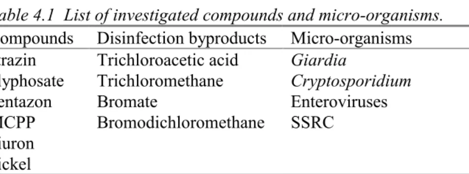
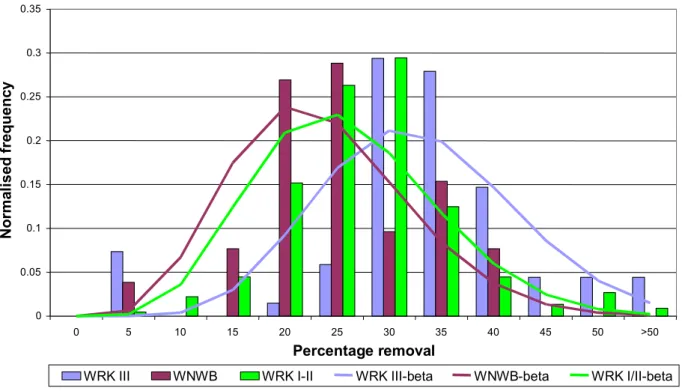
(21) RIVM rapport 734301 019. pag. 21 van 65. 4 Determination of removal percentages 4.1 Introduction In this chapter the so called percentages approach of the model is described. For each treatment step or combination of steps, data present in databases at RIVM, water companies and in the literature were collected to calculate removal percentages for micro-organisms and substances. This work resulted in percentage modules for treatment steps or combination of treatment steps based on ranges presented at the end of this chapter. The ranges make it possibel to use Monte Carlo simulation. A statistical appoach of the data of the production plants resulted in the use of a beta-distribution.. 4.2 Removal percentages based on data from databases and literature On the basis of information available at RIVM and in literature, single percentages and percentage ranges have been determined for the removal of substances and micro-organisms. The following information has been taken into account: • The so-called REWAB-module in ISDIV (the information system for drinking water and industrial water at the RIVM). This module contains information, delivered by the Dutch drinking-water companies, concerning the quality of water before, during and after drinking-water production. Unlike the company data mentioned above, this concerns figures aggregated over a year. • Literature relating to drinking-water treatment in the Netherlands. • Literature relating to drinking-water treatment outside the Netherlands. The aim was to find the minimum and maximum removal percentage for every combination of treatment step and substance. Based on expert judgement, improbable extremes have been skipped. In case of a choice of figures from several sources, priority has been given to company data over literature; literature concerning Dutch production plants has been given priority over literature concerning foreign plants. The results of this inventory are incorporated in the concluding table as shown in 4.2.. 4.3 Removal percentages based on data of drinking-water production plants The main part of the data that were used initially in the TAPWAT-project comprise of foreign, laboratory and pilot-scale data. Only a minor part of the data was based on full scale data of Dutch drinking-water production plants, whereas this type of data was considered to be the most important. For this reason, and also in order to obtain process, design and water quality parameters for modelling, additional data were obtained from a number of Dutch drinking-water production plants. Table 4.1 gives the list of compounds and micro-organisms that was investigated..

(22) pag. 22 van 65. RIVM rapport 734301 019. Table 4.1 List of investigated compounds and micro-organisms. Compounds Disinfection byproducts Micro-organisms atrazin Trichloroacetic acid Giardia glyphosate Trichloromethane Cryptosporidium bentazon Bromate Enteroviruses MCPP Bromodichloromethane SSRC diuron nickel Three calibration methods were applied. The first method is linear regression. The available measurement pairs are analyzed with the model Y = aX, with X and Y measurement values, and in the purification process the sampling point for X preceeds the sampling point for Y. The resulting point estimate for the parameter a has to be transformed to a removal percentage p by the formula p = 100 x (1 - a). The 95% confidence limits, that also have to be transformed by the same formula, will be taken as minimum and maximum borders for a removal percentage range, that can be used for Monte Carlo simulations, for instance. Values lower than 0% and higher than 100% will have to be corrected to 0% and 100%, respectively, to obtain realistic values that can be used e.g. for calculations of a complete purification process. The second method uses a (cumulative) distribution of removal percentages. First, the removal percentage p of each (X,Y)-pair is calculated (see also above). The removal percentage is set at -1E99 for measurement pairs where the inflow measurement equals zero. From the resulting set of removal percentages, the median or 50% percentile value is taken as a point estimate. For the minimum and maximum borders for a removal percentage range, the 2.5% and 97.5% percentile values are taken. The third method is applied when only one measurement pair is available. It comprises simply of calculation of the removal percentage for this measurement pair. Pathogenic micro-organisms For pathogenic micro-organisms the calculations were done with three data sets: • The original data set; • A set in which the inflow measurements that equal zero are set to 1; • A set in which the outflow measurements that equal zero are set to 1. Organic micropollutants and heavy metals If one or more measurements are below the detection limit, the calculations are performed with two data sets: • A set in which the inflow and outflow measurements that are below the detection limit are set to zero and the detection limit, respectively; • A set in which the inflow and outflow measurements that are below the detection limit are set to the detection limit and zero, respectively. Disinfection by-products For the chlorination step, a specific linear regression model has to be applied, since in this case there is no percentage removal, but formation of compounds. The general model applied is Y = a + X, where X and Y are the concentrations before and after chlorination,.

(23) RIVM rapport 734301 019. pag. 23 van 65. respectively. The parameter a represents the increase in disinfection byproduct concentration due to chlorination. For bromodichloromethane, the model is Y = a, since there is no information available on X. Also for the chlorination step, the cumulative distribution method is performed in analogy with the general description above, but using the set of concentration increases instead of removal percentages. In general, if one or more measurements are below the detection limit, the analysis is performed as described for organic micropollutants and nickel. Ranges The results of the present study are now used to obtain a table with ranges that can be used in a Monte Carlo analysis. For the lower and upper border of the range, the 2.5 and 97.5% percentile values are used or if necessary the values of the one pair method. For pathogenic micro-organisms, the point estimates of the percentiles are used, and for compounds the average is taken of the range for a percentile value. If values for two flows are available, then the average of these values is taken. Negative values are set to zero.. 4.4 Determination of removal percentages based on results of treatment plants The removal of compounds and micro-organisms and the formation of disinfection byproducts is summarized for different treatment steps of the following treatment plants: • WRK III-Water production location Prinses Juliana • WRK I/II-Water production location ir. Cornelis Biemond • WNWB-Zevenbergen • WBE-Kralingen • PWN-Andijk The complete set of results of the treatment plants are presented elswhere. The ranges are determined by the 2.5 and the 97.5 percentiles, for the lower and upper border of the range. The following basic principles have been applied in establishing the table: • Priority has been given to the ranges based on detailed company data (as described in 4.3), provided that the number of measurements used was sufficiently large to enable reasonably reliable results. • For turbidity and micro-organisms ranges have been compiled on the basis of detailed company data using the minimum and maximum removal as encountered in the individual treatment systems examined. In this way justice is done to the importance of peak amounts of micro-organisms for determining health effects. • For all other substances, ranges have been determined on the basis of detailed company data by taking the average median of the individual treatment systems and the average distance between the minimum and maximum removal with regard to the median. This method is based on the idea that for most substances the long term health effects are what matter and not incidental peaks. • Where no information based on detailed company data was available, use has been made of the ranges determined as described in 4.2..

(24) pag. 24 van 65. RIVM rapport 734301 019. The results used for the percentage modules of TAPWAT are presented in tabel 4.2 in the bold font. Ranges in regular font are based on literature and RIVM/TUD-data (i.e. the activities described in 4.2); ranges in bold font are based on detailed company data (i.e. the activities described in 4.3). Blanks indicate combinations of treatment step and substance/micro-organism for which no range could be determined.. 4.5 General conclusions from the data analysis Data availability • Due to the limited number of sampling points, not all purification steps can be analysed seperately. Coagulation/flocculation/sludge blanket separation + rapid filters is the most important example. • Of the five micro-organisms of interest, only data for spores of sulphite-reducing clostridia (SSRC) are available. • For the “organic micro-pollutants and heavy metals (six compounds) data availability is very limited and absent for two compounds. • Data availability is reasonable for disinfection by-products. Statistical analysis The non-normal nature of microbial counts and the high number of zero measurements makes linear regression and the percentile method, respectively, less useful. Application of an alternative statistical analysis, using e.g. the betabinomial approach (Teunis et al., 1997), could be useful. For organic micropollutants and heavy metals, a picture of broad ranges or zero emerges. This is caused by the very limited number of data pairs (1-2) in combination with measurements below the detection limit. The data for disinfection by-products are characterized by a reasonable number of measurement pairs and a limited number of measurements below the detection limit. This results in realistic estimates for the ranges of removal percentages and produced concentrations in the purification steps. Point estimates and ranges Useful point estimates and ranges of removal percentages (and produced concentrations) are only available for disinfection by-products. For organic micropollutants and nickel determination of point estimates and ranges is hampered by data availability and measurements below the detection limit. For SSRC, zero measurements is the main problem. Comparison with data from literature • • • .. The amount of overlap in the data of the present study and those collected from literature. The present study gives generally equal or lower values for removal percentages for corresponding cases, leading to a lowering of the percentages used for TAPWAT calculations for these cases. The comparison indicates that literature data (main part of previously collected data) might overestimate in general the removal that is realised in full scale drinking-water production plants..

(25) RIVM rapport 734301 019. pag. 25 van 65. Usefulness of full scale data for model calibration The usefulness of full scale data for model calibration is limited, due to limited data availability. These data are important, however, and should be used as much as possible for model calibration. Pilot-scale and laboratory data will have to fill in the (many) blanks..

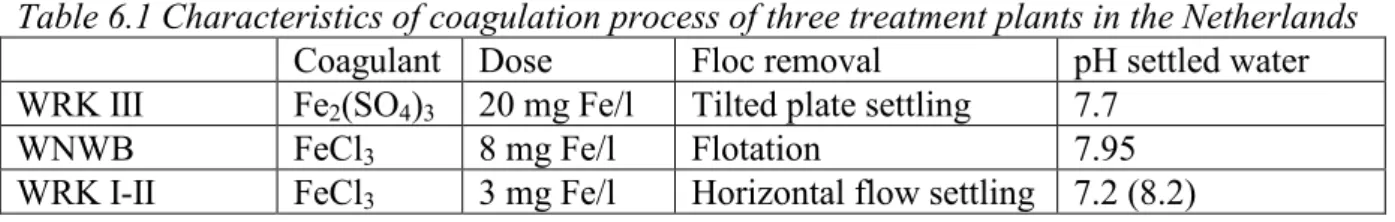
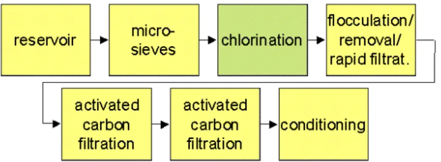
(26) RIVM rapport 734301 019. Conditioning. Chlorination. Safety chlorination ClO2 0-0 0-0 0-0 0-0 0-0 90-99.9 0-0 0-90 0-0. Microsieves. Coagulation/ Flocculation/ flocculation/ filtration* rapid filtration 0-20 0-20 20-20 20-20 20-82 20-82 60-93 60-93 20-60 -3.7-2.5 90-99 90-99 99-99.7 68.4-99.7 99-99.7 68.4-99.9 0-0 0-0 0-0 0-0 0-0 0-0. Atrazin 0-20 0-0 0-12.5 0-0 Diuron 0-25 0-0 0-0 0-0 Cadmium 60-80 0-0 0-0 0-0 Chromium 75-80 0-0 0-0 0-0 Nickel 0-0 0-0 0-0 0-0 Enteroviruses 99-99.9999 0-0 99-99.99 0-0 Cryptosporidium 68.4-99 0-0 0.76-5.8 0-0 Giardia 68.4-99 0-0 27-99 0-0 Bromate 0-0 0-0 0-0 0-0 Trichloromethane 40-85 0-0 0-0 Bromodichloro35-80 0-0 0-0 methane Simazin 0-0 0-0 0-0 0-0 0-0 0-20 0-20 Dimethoate 0-0 0-0 0-0 0-0 0-0 20-60 20-60 MCPA 0-0 0-0 0-0 0-0 0-0 60-60 60-60 MCPP 0-0 0-0 0-0 0-0 0-0 60-60 60-60 DOC 7.7-9.8 0-0 0-0 0-0 0-0 10-45 10.6-45.3 Tubidity 64-99.6 Trichloroacetic acid SSRC 0-100 96-99.9 *If applicable, the combination of treatment steps Coagulation/flocculation/rapid filtration should be used instead of the individual steps bold font: data are based on detailed company data regular font: data are based on RIVM/TUD data available.. Reservoir. Table 4.2 Removal percentages of compounds and micro-organisms and the formation of disinfection by-products expressed as ranges as used in TAPWAT 1.0.. pag. 26 van 65.

(27) Flocculation/ Sludge blanket Rapid filtration Slow sand flotation/ separation/ filtration rapid filtration* rapid filtration* 0-0 0-0 0-0 0-15 0-0 0-0 0-0 0-0 0-0 97-100 0-0 94-100 0-0 94-100 0-0 0-0 0-0. Infiltration / extraction. pag. 27 van 65. Ozonation. Atrazin 45-66 25-35 Diuron 73-73 Cadmium 15-50 0-0 Chromium 23-60 0-0 Nickel 25-60 0-0 Enteroviruses 99.9999-100 99-99.9 Cryptosporidium 94-100 45-79 Giardia 94-100 79-99 Bromate 0-0 0-0 Trichloromethane 75-99 0-0 Bromodichloro65-98 0-0 methane Simazin 0-35 0-0 45-68 20-27 Dimethoate 0-0 58-60 50-94 MCPA 0-3 90-99 90-99 50-75 MCPP 90-99 90-99 6.7-91 DOC 0-0 0-0 0-0 5.4-41.4 10.6-45.3 9.8-34.5 Tubidity 0-0 -169-98.2 64-99.6 46.8-97.4 Trichloroacetic acid SSRC 6-89.7 96-99.9 98-100 88.9-99.4 *If applicable, the combination of treatment steps Coagulation/flocculation/rapid filtration should be used instead of the individual steps bold font: data are based on detailed company data regular font: data are based on RIVM/TUD data available.. Flocculation /settling *. Table 4.2 continued.. RIVM rapport 734301 019.

(28) RIVM rapport 734301 019. Activated Aeration Hyperfiltration Nanofiltration Ultrafiltration Microfiltration carbon filtration Atrazin 20-90 0-0 90-99 65-98 0-0 0-0 Diuron 90-99 0-0 60-99 45-90 0-0 0-0 Cadmium 45-60 0-0 75-98 98-99 20-82 20-82 Chromium 40-70 0-0 72-96 96-99 60-93 60-93 Nickel 0-0 0-0 85-85 96-99 20-60 20-60 Enteroviruses 0-0 0-0 99.9-99.9999 99.99-99.99997 99-99.99997 90-99.9 Cryptosporidium 0-0 0-0 99.9-99.9997 99.99-99.9997 99.9-99.9997 99.99-99.999 Giardia 0-0 0-0 99.9-99.9997 99.99-99.9997 99.9-99.9997 99.99-99.999 Bromate 0-3.3 0-0 75-96 0-0 0-0 0-0 Trichloromethane 44-80 70-95 70-95 0-0 0-0 -239.4-33.0 Bromodichloro42-90 70-95 70-95 0-0 0-0 0-7.2 methane Simazin 35-90 0-0 78-95 65-95 0-20 0-20 Dimethoate 0-0 20-60 20-60 MCPA 50-99 0-0 75-99 75-98 60-60 60-60 MCPP 50-99 0-0 73-99 76-98 60-60 60-60 DOC 0-0 90-99 0-0 0-0 16.4-45.8 pH Tubidity Trichloroacetic acid SSRC bold font: data are based on detailed company data regular font: data are based on RIVM/TUD data available.. Tabel 4.2 continued. pag. 28 van 65.

(29) RIVM rapport 734301019. pag. 29 van 65. 5 Process or semi-empirical modelling 5.1 Introduction For the empirical modelling of the removal of pathogenic micro-organisms and the formation of disinfection by-products by chlorination and ozonation, a literature study has been done. The purpose of this literature study was to find models, which describes the relation between the design and process parameters of a certain treatment process and the removal (or formation) of a certain water quality parameter. In addition, several environmental parameters are considered which are directly or indirectly related to the removal or formation of the above mentioned parameters. The following treatment processes are considered: • Disinfection by chlorine • Disinfection by ozone The following parameters are considered: • Giardia • Cryptosporidium • Enteroviruses • Bromodichloromethane • Trichloroacetic acid • Temperature • Dissolved organic carbon • Acidity (pH) • Bromide. 5.2 Chlorination 5.2.1 Modelling the HOCl/OCl--equilibrium. The HOCl/OCL--equilibrium plays an important role in disinfection with chlorine. This is due to the fact that the disinfecting power of HOCl is much larger than that of OCl-. The pH is an important factor in the location of the equilibrium. Modelling the effect of the HOCl/OCL-equilibrium is derived from the classical Chick-Watson approach: ln(N/N0) = -k.CL2n.ContTime. In the case of a HOCl/OCl--solution the final formulae is 10 log(N/N0) = -k.loge.ContTime.(CL2/((H+)+Ka))n.((H+)n+a.Kan), in which Ka is a function of temperature (Haas, 1990): lnKa = 23.184-0.0583(Temp+273.15)-6908/(Temp+273.15) (H+) (HOCl) (OCl-) a Cl2 ContTime k Ka. H+-concentration (mol.l-1) HOCl-concentration (mg/l free chlorine) OCl--concentration (mg/l free chlorine) relative disinfection efficiency total free chlorine concentration (mg/l) contact time (min) disinfection rate constant (mg-n.ln.min-1) association constant (mol/l).

(30) pag. 30 van 65. N n N0 Temp. RIVM rapport 734301019. concentration micro-organisms (number/l) dilution coefficient concentration micro-organisms on time 0 (number/l) temperature (°C). 5.2.2 Giardia In modelling Giardia, a choice can be made from a number of articles of good quality. In Leahy et al. (1987), experimentally determined Ct99-values (Ct-values giving 99 % inactivation) for G. muris for 3 pH’s en two temperatures are presented; Further a Ct99analysis is made of G. lamblia-data of other researchers. In the complex of articles of Clark (1990), Clark and Regli (1993), Clark et al. (1989, 1990) and Smith et al. (1995) an empirical model is presented, incorporating the model of Chick-Watson and the variables temperature, pH, chlorine concentration and contact time. The parameters were determined using various articles with data on the influence of these variables. In Haas and Heller (1990) the models of Chick-Watson, Selleck and Hom were compared using experimental data on G. lamblia, for three pH’s and three temperatures, concluding that the model of Hom describes the data best. The parameters of the model of Hom at different pH’s and temperatures are given. It was decided to base the modelling in first instance on the complex of articles of Clark (1990), Clark and Regli (1993), Clark et al. (1989, 1990) and Smith et al. (1995), as in these articles the largest number of variables (temperature, pH, chlorine concentration and contact time) is taken into consideration. Leahy et al. (1987) restricted themselves to Ct-modelling. Haas and Heller (1990) did use the more flexible model of Hom, but they did not model pH and temperature. Within the complex of articles mentioned above the most recent article, that of Smith et al. (1995) was chosen. From Smith et al. (1995) it is not clear what C exactly is: the dose, the rest concentration or something different. A conservative approach is to assume that it is the restconcentration: Cl2 = Cl2-Rest. In the equation depends the removal of Giardia on the initial and the rest concentration of chlorine, the contact time, the temperatue and the pH. There is an equation for temperatures below and one for temperatures above 12.5 °C.. 5.2.3 Cryptosporidium The module for Cryptosporidium is based on Korich et al. (1990) who use the Ct-concept. In chlorine free water (which implies in principle a constant chlorine concentration) a Ct99value was measured of 7200 mg.min.l-1 which leads to a value for k of 6.396.10-4 l.mg-1.min-1. This concept can be extended to a temperature correction and a correction can be applied for the HOCl/OCl- equation. If in the experiments of Korich et al. (1990) the chlorine concentration is indeed constant, in principle the above value for k can be used in a model formulation in which the concentration chlorine decreases exponentially. This leads to replacing the factor Cl2 with the expression Cl2 Dose(e-v.Time-1). The considerations above lead to an equation in which the course of the Cl2 concentration, contact time, temperature and pH play a role..

(31) RIVM rapport 734301019. pag. 31 van 65. 5.2.4 Enterovirus In Medema and Theunissen (1996), Sobsey et al. (1991) is used. Their Ct99.99-values are given for 3 pH’s. pH Ct (mg.l-1.min) (free available chlorine) 6 2.3 8 2.0 10 19.3 On the basis of these data the inactivation was modelled according to the Ct-approach, extended with the Q10-approach for temperature. In the literature it was concluded that the model of Chick-Watson satisfies the best. log(EntvirOut/EntvirIn) = -k.Cl2.ContTime.2(Temp-5)/10loge The Chick-Watson-parameters (k, n) are given for 2 pH’s and four temperatures. For the effect of pH, the equation which uses the HOCl/OCl--equilibrium, is used. For viruses n=1 en a=0.004 in this equation (Chang, 1971). For experimental data Sobsey et al. (1991) is used. A conservative approach is used which implies that from the three Ct-values at different pH’s given there the most conservative value is chosen as starting value for the calculations, with which the value of k is calculated. It can be reasoned that the Ct-waarde at pH=6 is the most conservative one and this one was used in first instance for modelling. The value of k was calculated using the HOCL/OCL--equations and equals 4.0735 mg-1.l.min. During validation in a later stage it appeared that this value could not be maintained and it was calibrated for the situation in practice to 0.212 mg-1.l.min-1. In summary, the model is extended with a factor ((H+)+a.Ka)/((H+)+Ka), in which k = 0.212 mg-1.l.min-1, a=0.004 and lnKa = 23.184-0.0583(Temp+273.15)-6908/(Temp+273.15) In the experiments of Sobsey et al. (1991) the mean of the initial and final concentration is used for the concentration of chlorine. We must choose here for incorporation in a model in which the rest concentration is used or a model in which the decrease in concentration is incorporated. The mean as a measure for concentration implies that translation to rest concentration gives a larger underestimation for the disinfecting action than translation to a “decrease model”. This is why the last option is chosen. The final formulae then becomes analogous to the equation for Cryptosporidium.. 5.2.5 Trichloromethane Three relevant articles were found on the formation of tricholoromethane (TCM or chloroform) is subject namely of Alekseeva et al. (1987), Clark et al. (1996) and Singer (1993). Alekseeva et al. (1987) presented an empirical model with variables COD, pH, chlorine concentration and contact time, using also the interaction terms between these variables. In Clark et al. (1996) the variables pH, time, chlorine- and bromide concentration were considered. Singer (1993) presents a model in which all variables are risen to a power and subsequently multiplied with each other. The variables are TOC (total organic carbon) and UV-254 (absorption of ultraviolet light at 254 nm) (both as surrogate parameters for disinfection by-products (DBP- precursors), pH, chlorine dosis, contact time, temperature and bromide concentration..

(32) pag. 32 van 65. RIVM rapport 734301019. In summary, all these authors incorporated pH, chlorine concentration and contact time in their modelling. Only Singer (1993) used in addition temperature and therefore this model will be applied here. The model of Singer (1993) contains three variables (TOC, UV-254 and bromide) that were in first instance not incorporated in the first fase of TAPWAT. Assuming that there is hardly a difference DOC is substituted for TOC in the model of Singer (1993). For the values of UV-254 and bromide, an estimation was made on the basis of REWAB-data (mean values) for the years 1992 up to and including 1995 for Andijk, RotterdamBeerenplaat, Rotterdam-Kralingen and Amsterdam-Leiduin. The mean of intake and finished water should be considered as an estimation of the water quality of the oxidation process, which is situated somewhere between intake and finished water. The resulting values are: • UV-254 = 0.0655 cm-1 • bromide = 0.1635 mg/l Not incorporating bromide was in addition justified by an analysis of the minimum- and maximum values in the years and for the purification plants mentioned above. Substitution of the lowest and highest values found (0.050 en 0.52 mg/l) in the model of Singer (1993) gives a ratio between extreme TCMout-values of 2.3. This can be compared with an a priori acceptable ratio of 5 (pers.comm. Versteegh), which justifies not incorporating bromide in the model equation. This leads to the following equation: TCMOut = k1 ⋅ DOC k2 CL2_ Dose k3ContTime k4 Temp k5 (PH − k6) k7 with k1 = 0.037 (complexe dimensie), k2 = 0.616, k3 = 0.391, k4 = 0.265, k5 = 1.15, k6 = 2.6, k7 = 0.800 and TCMOut = Trichloromethane concentration in outflow (µg/l) DOC = Dissolved Organic Carbon (mg/l) CL2 dose = Dose chlorine concentration (mg/l) ContTime = Contact time (hours) Temp = Temperature (°C) PH = pH. 5.2.6 Bromodichloromethane For chlorination and the formation of bromodichloromethane (BDCM) the situation is analogous to chlorination and the formation of trichloromethane, the only difference being that Alekseeva et al. (1987) did not work on bromodichloromethane. In the model of Singer (1993) is substituted UV-254 = 0.0655 cm-1, Bromide = 0.1635 mg/l and DOC for TOC. Not incorporating bromide is justified by an analysis analogous to trichloromethane which gives a ratio between extreme BDCMout-values of 1.3 which in turn justifies not incorporating bromide in the model equation. The equation is analogous to that for trichloro methane with TCMOut replaced by BDCMOut (Bromodichloromethane in outflow (µg/l)). The parameter values are: k1 = 0.594 (complex dimension), k2 = 0.177, k3 = 0.309, k4 = 0.271, k5 = 0.720, k6 = 2.6, k7 = 0.925..

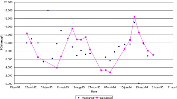
(33) RIVM rapport 734301019. pag. 33 van 65. 5.2.7 Trichloroacetic acid For chlorination and the formation of trichloroacetic acid (TCA) the situation is analogous to chlorination and the formation of trichloromethane, the difference being that Alekseeva et al. (1987) did not work on TCA and that the model of Singer (1993) does not incorporate temperature for this compound. Further, TOC and UV-254 are not in the formula for TCA as a product, but as separate variables. In the model of Singer (1993) is substituted UV-254 = 0.0655 cm-1, Bromide = 0.1635 mg/l and DOC for TOC. Not incorporating bromide was justified by an analysis analogous to trichloromethane which results in a ratio between extreme TCAout-values of 1.3 which in turn justifies not incorporating bromide in the model equation. This leads to the following equation: TCAOut = k1 ⋅ DOC k2 CL2_Dose k3ContTime k4 pH k5. TCAOut = Trichloroacetic acid in outflow(µg/l) For a description of the other variables one is referred to trichloromethane. k1 = 73.4 (complex dimension), k2 = 0.355, k3 = 0.881, k4 = 0.264, k5 = -1.732. As a result of calibration, it proved necessary to replace the original value of k1 (based on the work of Singer) with the value above.. 5.2.8 Verification of formation of trichloromethane by chlorination In paragraph 5.2.5 the formulae for the prediction of the formation of trichloromethane are summarised. For the prediction of trichloromethane formation by chlorination the adapted model of Singer (1993) is used:. TCM out = 0.037 * (TOC ) 0.616 * Cl 2 dose 0.391 * ContTime 0.265 * Temp 1.15 K * ( pH − 2.6) 0.8 where, TCMOut TOC CL2 dose ContTime Temp pH. = Trichloromethane concentration in outflow (µg/l) = Total Organic Carbon (mg/l) = Chlorine dose (mg/l) = Contact time (hours) = Temperature (°C) = pH. Data from WNWB-Zevenbergen and PWN-Andijk are used for the validation of this formula. At these plants chlorination takes place for disinfection purposes. The results are shown in the figures 5.1 and 5.2. Visual interpretation of the graph leads to the conclusion that the prediction of the formation of trichloromethanes at Zevenbergen is rather good, in accordance to the prediction of the first year at Andijk. The results of the second year at that pumping station give a high overestimation of practice. This is mainly due to the fact that in this period sodiumbisulfite is.

(34) pag. 34 van 65. RIVM rapport 734301019. dosed at the end of the contact tanks, which takes out the chlorine and thus reduces the contact time and consequently the formation of trichloromethanes. Trichloromethane formation at Zevenbergen 20.000 18.000 16.000. TCM (mug/l). 14.000 12.000 10.000 8.000 6.000 4.000 2.000 0.000 15-jul-92. 23-okt-92. 31-jan-93. 11-mei-93. 19-aug-93. 27-nov-93. 07-mrt-94. 15-jun-94. 23-sep-94. 01-jan-95. 11-apr-95. Date measured. calculated. Figure 5.1 Example 1 of a validation of the module chlorination. Trichloromethane formation at PWN-Andijk 35.00. 30.00. TCm (mug/l). 25.00. 20.00. 15.00. 10.00. 5.00. 0.00 09/23/94. 01/01/95. 04/11/95. 07/20/95. 10/28/95. 02/05/96. 05/15/96. 08/23/96. 12/01/96. 03/11/97. date caluculated. measured kad. measured za10. Figure 5.2 Example 2 of a validation of the module chlorination Further it can be concluded from the data of PWN-Andijk (and Zevenbergen) that there is a retardation in the prediction. It is uncertain which is the cause of it, but for the model TAPWAT this is not relevant. It is mainly of importance that a certain concentration peak is predicted and the exact time of the occurrence not..

(35) RIVM rapport 734301019. pag. 35 van 65. 5.3 Ozonation 5.3.1 Giardia In Medema and Theunissen (1996), the data of Finch et al. (1993a) are used. In there the inactivation was determined for a range of five Ct values. Based on these data, the inactivation was modelled according to the Ct-concept, extended with the Q10 approach for temperature. Finch et al. (1993a) calculated parameters of the model of Hom. This application of the model of Hom was coupled to the assumption of an exponential decrease of the ozone concentration with time. This is a somewhat curious approach, as a very empirical equation is combined with a process description approach. Therefore it was decided to perform an analogous calculation of the parameters of the model of Hom as in Finch et al. (1993b) in order to apply this model in the first phase of TAPWAT. Finch et al. (1993a) used the ozone residual for the ozone concentration for an analysis of the data according to the Ct-concept; For this reason this will be done also in this model formulation (OZ = OZ-rest). At least squares fitting was done with the model of Hom and the data of Finch et al. (1993a). For TAPWAT the model of Hom, extended with a temperature correction, can be reformulated into the following equation.. Temp − k4 k5 − k1 ⋅ OZ - Rest k2 ContTime k3 + 1 2 loge GiardiaOut = GiardiaIn ⋅ 10 met k1 k2 k3 k4 k5 GiardiaOut GiardiaIn OZ-Rest ContTime Temp. k3 + 1. = Disinfection rate constant k = 2.229 mg-k2.lk2.min-(k3+1) = Dilution coefficient n = 0.138(-) = Homcoefficient m = -0.560 (-) = base temperature for temperature effect = 22 °C = temperature rise for doubling the disinfection rate = 10 °C = Concentration Giardia in outflow (number/l) = Concentration Giardia in inflow (number/l) = Rest concentration ozone (mg/l) = Contact time (min) = Temperature (°C). 5.3.2 Cryptosporidium Medema and Theunissen (1996) used the data of Finch et al. (1993b). In there a large dataset on ozone inactivation of Cryptosporidium is presented. Based on these data the inactivation was modelled according to the Ct-concept, extended with the Q10 approach for temperature. Finch et al. (1993b) calculated the parameters of the model of Hom for two temperatures. Finch et al. (1993b) used the so-called ‘integrated ozone residual’ as a measure for the ozone concentration. This is a geometric mean of initial and final concentration. The parameter.

(36) pag. 36 van 65. RIVM rapport 734301019. values calculated by Finch et al. (1993b) can be used for application of the model of Hom combined with exponentially decreasing disinfectant concentration. This model is not analytically solvable. Application of this model is possible using numerical integration. This modelling approach is somewhat curious however, as a very empirical formula is combined with a process description approach. Therefore now the model of Hom is applied with a constant disinfectant concentration. For OZ the rest concentration is substituted (OZ = OZ-rest) and the formula is extended with a temperature correction. The parameters of Hom at 7 °C were used. The resulting equation is analogous to the equation for Giardia, with GiardiaOut en GiardiaIn replaced by CryptoOut and CryptoIn, respectively, the concentration Cryptosporidium in outflow and inflow (number/ml). The parameter values are: k1 k2 k3 k4 k5. = Disinfection rate constant k = Dilution coefficient n = Hom coefficient m = base temperature for temperature effect = temperature rise for doubling the disinfection rate. = 0.634 mg-k2.lk2.min-(k3+1) = 0.68(-) = -0.05 (-) = 7 °C = 15 °C. 5.3.3 Enterovirus Medema and Theunissen (1996) used the data of Roy et al. (1980). In this article data are presented on well performed experiments on the effects of concentration, contact time, pH and temperature on the inactivation of poliovirus 1. Modelling was performed based on these data, using the Ct and the Q10 approach. Herbold et al. (1989) determined the parameters of an exponential inactivation model at different ozone concentrations and temperatures for hepatitis A virus and poliovirus 1. As the model information in this article does not lead to improvement or extension of the model formulation, it was decided in first instance to apply the approach of Medema and Theunissen (1996). In the experiments of Roy et al. (1980) the ozone concentration was kept constant during the exposure time using a continuous flow reactor. In this situation the value of k (see parameter list) can be determined. It equals 20.93 mg-1.l.min-1.. In principle this same value of k can be applied in a model formulation in which the concentration of ozone declines exponentially. However, from a validation procedure it appeared that this value had to be changed for the situation in practice to 0.799 l.mg-1.min-1. The above leads to the following model: æ k1 ö logeç ÷OZ - Doseæç e − k4 ⋅ ContTime − 1ö÷2 è ø è k4 ø EntvirOut = EntvirIn ⋅ 10. Temp − k2 k3. k4 follows from the dose, rest concentration and the contact time, according to OZ_Rest = OZ-Dose.e-k4.ContTime, so that.

(37) RIVM rapport 734301019. pag. 37 van 65. æ OZ - Rest ö − lnç ÷ OZ - Dose ø è k4 = ContTime k1 = Disinfection rate constant k = 0.799 l.mg-1.min-1 k2 = base temperature for temperature effect = 5 °C k3 = temperature rise for doubling the disinfection rate = 10 °C -1 k4 = Disappearing rate constant v (min ) EntvirOut = Concentration virus in outflow (number/l) EntvirIn = Concentration virus in inflow (number/l) OZ_Dose = Dose concentration ozone (mg/l) OZ_Rest = Rest concentration ozone (mg/l) ContTime = Contact time (min) Temp = Temperature (°C). 5.3.4 Bromate On modelling bromate formation during ozonation two relevant articles were found. Schmidt et al. (1995) give a model with variables ozone, DOC and bromide. Song et al. (1996) modelled the variables bromide, DOC, ammonia-nitrogen, ozone, pH, alkalinity and reaction time. Because of the modelling of pH and reaction time, the model of Song et al. (1996) was chosen. The model of Song et al. (1996) contains three variables (bromide, ammonia-nitrogen and alkalinity) that were in first instance not modelled in the first phase of TAPWAT. Therefore an estimation was made for the values of bromide, ammonia-nitrogen and alkalinity, using the same data and approach as for trichloromethane. For the calculation of alkalinity the formule in Schock (1990) was used: • Total alkalinity = (HCO3-) + 2(CO32-) + (OH-) - (H+) • The resulting values are: • bromide = 0.1635 mg/l • NH4-N = 6.5528 mg/l • alkalinity = 215.5631 mg CaCO3/l The incorporation of bromide was further investigated by an analysis analogous to trichloromethane, which gives a ratio between extreme bromate concentrations of 7.9, which in turn implies that bromide has to be incorporated into the model formulation. This results in the following equation. Bromate = k1 ⋅ DOC k2 OZ - Dose k3PH k4 ContTime k5 Bromide k6. with k1 = 1.46.10-6 (complex dimension), k2 = -1.18, k3 = 1.42, k4 = 5.11, k5 = 0.27, k6 = 0.88 and Bromate = Bromate (µg/l) DOC = Dissolved Organic Carbon (mg C/l) OZ_Dose = Dose ozone concentration (mg/l) PH = pH (-) Alkalinity = alkalinity (mg CaCO3/l) ContTime = Contact time (min) Bromide = bromide (µg/l) = ammonia-nitrogen (mg N/l) NH3-N.

(38) pag. 38 van 65. RIVM rapport 734301019. 5.4 Conclusions The formulae, presented in this chapter, are based on many observations. The validation for Dutch circumstances only is tested. As can be seen in paragraph 5.2.8, this is done for the formation of trichloromethane after chlorination. In TAPWAT the modules chlorination and ozonation are incorporated for the prediction of disinfection by-products. The result of the empirical models is a point estimate for the formation of disinfection byproducts and the distribution in the input data will therefore directly be transferred to the output. No extra uncertainty is introduced in this module..

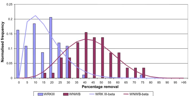
(39) RIVM rapport 734301019. pag. 39 van 65. 6 Stochastic modelling of the removal of natural organic compounds in drinking-water processes 6.1 Introduction In the preceding chapters, the removal and formation of compounds and the removal of organisms is determined by empirically determined removal percentages (and ranges) and by point estimates based on regression analyses of the performance of treatment plant in the USA. The disadvantage of point estimates is that it is not clear what is the confidence interval of the calculated value. In design and operation of modern drinking-water production processes it is necessary to perform probabilistic modelling. As formulated by Haarhoff (Haarhoff, 2000): ”For models that will be increasingly used for optimization, it is essential that predictions are formulated in probabilistic terms. Designers and operators need not only know the average performance of a process, but are specifically interested in the tails of the performance distribution, as good performance has to be maintained under extreme conditions. This requirement becomes quite evident when the performance of a system has to be predicted, given the performance of the individual processes making up the system”. With test data statistical techniques are used to construct an appropriate model and to estimate its parameters. Once a model is obtained, it may, of course, be used to predict future performance (Hahn, 1967). For the determination of the statistical distribution of removal percentages by a specific process, different models can be used. For the removal or organic compounds the ”beta-distribution” is chosen, because of its continuous character and its flexibility in shape in the range between 0 and 1 (0-100%).. 6.2 Removal of organic compounds in conventional drinkingwater treatment processes In conventional treatment plants natural organic compounds are only removed by floc formation/removal and by activated carbon (filtration). NOM may cause colour, is a precursor for disinfection by-products, can compete with adsorption sites for pesticides and VOC’s (Kruithof 1994; Sorial, 1994; Summers, 1993, Hopman, 1991) and can promote microbial growth and fouling of membranes. Floc formation and removal. Dennet (Dennet, 1996) reviewed several articles and did some research (jar-tests) on concentrated river and lake water. The effectiveness of coagulation for removing NOM depends on charge, solubility and molecular-size characteristics. The efficiency of removing organic carbon is proportional to molecular size, with larger-molecular-weight components more effectively removed than smaller ones. Sinsabaugh (Sinsabaugh, 1986) determined that acidic and basic components of the NOM in natural waters were twice as likely to be removed by coagulation as non polar neutral compounds. The removal of neutral compounds depended on their polarity and the availability of low-polarity sorption sites on the floc. (Phylic and phobic compounds were precipitated more readily than mesics)..

No results found