Manual of FOCUS PEARL version 1.1.1 | RIVM

Hele tekst

(1)research for man and environment. RIJKSINSTITUUT VOOR VOLKSGEZONDHEID EN MILIEU NATIONAL INSTITUTE OF PUBLIC HEALTH AND THE ENVIRONMENT. RIVM report 711401 008, Alterra report 28 Manual of FOCUS PEARL version 1.1.1 A. Tiktak, F. van den Berga, J.J.T.I. Boestena, D. van Kraalingena, M. Leistraa and A.M.A. van der Linden November 2000. a) Co-authors from Alterra Green World Research. This investigation has been performed by order and for the account of: − The Directorate-General of the RIVM, within the framework of RIVM project 711401, Soil and Groundwater Models. − Ministry of Agriculture, Nature Management and Fisheries, within the framework of Research programme 359, Pesticides and the Environment RIVM, P.O. Box 1, 3720 BA Bilthoven, telephone: +31 30 2749111; telefax: +31 30 2742971 ALTERRA Green World Research, Wageningen University and Research Center, PO BOX 47, 6700 AA Wageningen, The Netherlands, telephone +31 317 474202; telefax: +31 317 424812.

(2) page 2 of 144. RIVM report 711401 008. © 2000 RIVM, Alterra No part of this publication may be reproduced in any form or any means, or stored in a database or retrieval system, without the written permission of RIVM and Alterra RIVM and Alterra assume no liability for any losses resulting from the use of this document and from the use of the software documented in this report..

(3) RIVM report 711401 008. page 3 of 144. Abstract The PEARL model is used to evaluate the leaching of pesticide to the groundwater in support to the Dutch and European pesticide registration procedures. PEARL is an acrononym for Pesticide Emmission Assessment at Regional and Local scales. The model is a joint product of Alterra Green World research and the National Institute of Public Health and the Environment, and it has replaced the models PESTLA and PESTRAS since June 1st, 2000. Model and data can be accessed through a user-friendly Graphical User Interface for Windows 95/98/NT. All data are stored in a relational database. Both the Dutch standard scenario and the European standard scenario’s as suggested by the FOCUS modeling working group can be accessed through the User Interface. This report gives a description of the processes and parameters included in PEARL version 1.1. It also contains a description of the Pearl User Interface and the input and output files. The Dutch standard scenario is described briefly. Keywords: Pesticides; leaching; groundwater; soil; risk-assessment; interface. PEARL; FOCUS;. graphical user.

(4) page 4 of 144. RIVM report 711401 008.

(5) RIVM report 711401 008. page 5 of 144. Preface Pesticide leaching models have been developed and used in The Netherlands since the early seventies, but their use in pesticide registration was limited until 1989. In that year the PESTLA (PESTicide Leaching and Accumulation) model was launched and officially incorporated in the evaluation process. Initially, its use was limited to estimate leaching under standard soil and weather conditions in the first tier of the evaluation process, but within a few years its use was extended to higher tier assessments and evaluations outside the registration process. The broader use stimulated the release of new versions of PESTLA, but also the development of the PESTRAS (PESTicide TRansport ASsessment) model; the latter especially developed for regional-scale applications. Although the description of pesticide behavior in both models was based on PESTLA, the two models produced different results. Although the differences were small, they were significant at the leaching level of 0.1 g ha-1, which is relevant in the registration process. As this was considered unacceptable, the Ministry of Agriculture, Fisheries and Nature Preservation (LNV) and the Ministry of Housing, Spatial Planning and the Environment (VROM) charged Alterra Green World Research and the National Institute of Public Health and the Environment (RIVM) with the development of a consensus leaching model. In 1997, a project team was formed to develop the new model. The team consisted of the authors of this report. The project team decided that PEARL (Pesticide Emission Assessment at the Regional and Local scale) should be more than a simple merger of the two precursors. The opportunity was taken to: − include recent scientific developments − upgrade the computer language to FORTRAN 95 and make use of object oriented techniques − develop an object oriented database to assist in generating input and archiving − develop a graphical user interface, called PUI (Pearl User Interface), consistent with the database, for easy use of the software. Francisco Leus and Klaas Groen (RIZA) commented in the early stages on the concepts to be included in PEARL. Bernd Gottesbüren (BASF) and Helmut Schäfer (Bayer) reviewed the draft manuscripts and tested the software package. Their contributions are gratefully acknowledged. The software package contains an e-mail address for communication with the developers. Users of PEARL are encouraged to report difficulties and errors they experience as well as suggestions for improvement..


(7) RIVM report 711401 008. page 7 of 144. Contents List of Symbols and Units. 11. Samenvatting. 15. Summary. 17. 1. Introduction. 19. 1.1. General introduction. 19. 1.2. Accompanying reports. 20. 1.3. Reporting of errors. 21. 1.4. Structure of report. 21. 2. Model description. 23. 2.1. Overview. 23. 2.2. Vertical discretization. 24. Hydrology. 25. 2.3.1 2.3.2 2.3.3 2.3.4 2.3.5 2.3.6 2.3.7 2.3.8. 25 26 27 27 28 28 28 29. 2.3. 3. Soil water flow Potential evapotranspiration Potential transpiration and potential evaporation Uptake of water by plant roots Evaporation of water from the soil surface Interception of rainfall Bottom boundary conditions Lateral discharge of soil water. 2.4. Heat flow. 30. 2.5. Pesticide fate. 31. 2.5.1 2.5.2 2.5.3 2.5.4 2.5.5 2.5.6 2.5.7 2.5.8 2.5.9 2.5.10. 31 31 32 32 34 34 35 37 39 39. Pesticide application Canopy processes Mass balance equations Transport in the liquid phase Transport in the gas phase Initial and boundary conditions Partitioning over the three soil phases Transformation of pesticide in soil Pesticide uptake Lateral discharge of pesticides. Model parameterization. 41. 3.1. Hydrology. 41. 3.1.1 3.1.2 3.1.3 3.1.4. 41 44 44 45. Soil water flow Potential evapotranspiration Uptake of water by plant roots Evaporation of water from the soil surface.

(8) page 8 of 144. RIVM report 711401 008. 3.1.5 3.1.6. 3.2. 4. 45 45. Pesticide fate. 45. 3.2.1 3.2.2 3.2.3 3.2.4 3.2.5 3.2.6 3.2.7 3.2.8 3.2.9 3.2.10 3.2.11. 45 47 47 47 48 48 50 50 51 51 54. Compounds and transformation scheme Pesticide application Initial and boundary conditions Transport in the liquid phase Transport in the gas phase Freundlich equilibrium sorption Freundlich non-equilibrium sorption Gas-liquid phase partitioning Transformation of the compound Transformation of the compound in case of sorption/desorption kinetics Compound uptake. User’s guide for the command line version of PEARL. 55. 4.1. Running the model. 55. 4.2. Description of the PEARL file. 56. 4.2.1 4.2.2 4.2.3 4.2.4 4.2.5 4.2.6 4.2.7 4.2.8 4.2.9 4.2.10 4.2.11 4.2.12 4.2.13 4.2.14. 56 58 59 60 60 61 63 64 65 68 68 69 70 71. Structure of records in the PEARL input file General rules for variable names Getting started with the command-line version Overview of sections in the PEARL files Section 1: Simulation control Section 2: Soil properties and soil profile Section 3: Weather and irrigation data Section 4: Boundary and initial conditions of the hydrological model Section 5: Compound properties Section 6: Management Section 7: Initial and boundary conditions Section 8: Crop properties Section 9: Control of daily output Description of the weather data file. 4.3. Description of the irrigation data file. 72. 4.4. Description of the comprehensive output file. 73. 4.4.1 4.4.2 4.4.3. 73 74 74. 4.5. 5. Interception of rainfall Bottom boundary conditions. Output as a function of time Vertical profiles of some selected variables Importing data in Excel. Description of the summary output file. 75. 4.5.1 4.5.2 4.5.3. 75 77 77. Annual balances FOCUS output Summary variables for the Dutch pesticide registration procedure. User’s guide for the PEARL user interface. 79. 5.1. Overview of the PEARL database. 80. 5.2. Getting started. 82. Generating FOCUS runs. 82. 5.3.1 5.3.2 5.3.3 5.3.4 5.3.5. 83 83 84 84 84. 5.3. Create or edit a substance Create or edit one or more application scheme(s) Run the FOCUS wizard Refinement Running PEARL.

(9) RIVM report 711401 008. 5.3.6. page 9 of 144. Viewing the Results. 5.4. General properties of the PEARL user interface. 85. 5.5. The projects form. 86. 5.6. The main form. 86. 5.6.1 5.6.2. 87 87. 5.7. 5.8. 5.9. The main menu The tabs of the main form. Editing locations. 88. 5.7.1 5.7.2 5.7.3 5.7.4 5.7.5. 88 90 91 92 93. The locations form The soil form The soil building blocks form The meteo form Boundary conditions of the hydrological model. Editing crop calendars. 95. 5.8.1 5.8.2. 95 96. The crop calendar form The crop and development stage form. Editing substances 5.9.1 5.9.2. Editing individual compounds The transformation scheme form. 5.10 Editing application schemes 5.10.1 5.10.2. Application schemes Applications. 98 98 101. 102 102 102. 5.11 Editing irrigation schemes. 103. 5.12 Defining the output of the model. 104. 5.12.1 5.12.2. The output control tab of the main form The detailed output options form. 104 104. 5.13 Running the model. 106. 5.14 Creating graphs. 106. 5.14.1 5.14.2 5.14.3. 6. 84. Working with predefined graphs Working with user-defined graphs The XYWIN program. 107 109 109. 5.15 The FOCUS wizard. 110. 5.16 Installation, support and registration. 113. The Dutch standard scenario. 115. 6.1. Parameterization. 115. 6.1.1 6.1.2 6.1.3 6.1.4. 115 116 116 116. Soil properties Meteorological conditions Crop properties Compound properties. 6.2. Running the Dutch standard scenario. 117. 6.3. Results. 117. References Appendix 1. 123 Mailing list. 127.

(10) page 10 of 144. RIVM report 711401 008. Appendix 2. The PEARL input file – Expert users. 131. Appendix 3. Manual of PEARLNEQ. 141.

(11) RIVM report 711401 008. page 11 of 144. List of Symbols and Units Symbol a aC,g aC,L ag aM,g aM,L aT,L aT,g Ap Ad,p Ad,f Ad,s bg B bC,g bC,L bM,g bM,L bT,g bT,L ca Ca Cclay c*eq c*ne C(h) Ch cg cg,0 cg,1 cL cL,r Com Csand Cw da ds Da Da,r Ddif,g Ddif,L Ddis,L DT50,r Dw Dw,r Ea Emax. Description interception coefficient coefficient in Currie diffusion equation for the gas phase coefficient in Currie diffusion equation for the liquid phase parameter in bottom flux-phreatic head relationship exponent in numerator of Millington equation for gas phase exponent in numerator of Millington equation for liquid phase coefficient in Troeh diffusion equation for the liquid phase coefficient in Troeh diffusion equation for the gas phase Areic mass of pesticide at the crop canopy Areic mass deposited on the plants Areic mass deposited on the field Areic mass deposited on the soil surface parameter in bottom flux-phreatic head relationship exponent for the effect of soil moisture on transformation exponent in Currie diffusion equation for the gas phase exponent in Currie diffusion equation for the liquid phase exponent in denumerator of Millington equation for gas phase exponent in denumerator of Millington equation for liquid phase exponent in Troeh diffusion equation for the gas phase exponent in Troeh diffusion equation for the liquid phase concentration in air volumic heat capacity of water volumic heat capacity of clay pesticide concentration in the equilibrium domain of the soil pesticide concentration in the non-equilibrium domain of the soil differential water capacity volumic heat capacity concentration in the gas phase concentration in the gas phase at the soil surface concentration in the gas phase in center of top layer concentration in the liquid phase reference concentration in the liquid phase volumic heat capacity of organic matter volumic heat capacity of sand volumic heat capacity of water thickness of air boundary layer thickness of soil boundary layer pesticide diffusion coefficient in air pesticide diffusion coefficient in air at reference temperature coefficient of pesticide diffusion in the gas phase coefficient of pesticide diffusion in the liquid phase coefficient of pesticide dispersion in the liquid phase half-life in equilibrium domain at reference temperature pesticide diffusion coefficient in pure water pesticide diffusion coefficient in water at reference temperature molar enthalpy of transformation maximum soil evaporation flux based on Darcy equation. Unit m m d-1 m3 m-3 m3 m-3 m d-1 kg m-2 kg m-2 kg m-2 m-1 kg m-3 J m-3 K-1 J m-3 K-1 kg m-3 kg m-3 m-1 J m-3 K-1 kg m-3 kg m-3 kg m-3 kg m-3 kg m-3 J m-3 K-1 J m-3 K-1. Acronym CofIntCrp CofDifGasCur CofDifLiqCur CofFncGrwLev ExpDifGasMilNom ExpDifLiqMilNom CofDifLiqTro CofDifGasTro AmaCrp AmaAppCrp AmaApp AmaAppSol ExpFncGrwLev ExpLiqTra ExpDifGasCur ExpDifLiqCur ExpDifGasMilNom ExpDifLiqMilNom ExpDifGasTro ExpDifLiqTro ConAir NR NR ConSysEql ConSysNeq NR NR ConGas ConGasUbo ConGas(1) ConLiq ConLiqRef NR NR. m m m2 d-1 m2 d-1 m2 d-1 m2 d-1 m2 d-1 d m2 d-1 m2 d-1 J mol-1 m3 m-2 d-1. ThiAirBouLay ThiLay(1)/2 CofDifAir CofDifAirRef CofDifGas CofDifLiq CofDisLiq DT50Ref CofDifWat CofDifWatRef MolEntTra NR.

(12) page 12 of 144. Symbol ETr Es Ep ETp ETp0 ETw0 fc fd fd,p fd,s fm fK,ne ft fu fw h H h1..h4 Jp,g Jp,L Jp,v Jv,a Jv,s Jw,p Ka kd kdsp KF,eq KF,eq,r KF,ne KH K(h) Kom,eq Ks kt kt,par kt,p kvol LAI Ldis,L Lk Lroot M N n m mom P Pi Pmin. Description reference evapotranspiration according to Makkink actual flux of evaporation from the soil potential flux of evaporation from the soil potential evapotranspiration flux idem, of a dry canopy, completely covering the soil idem, of a wet canopy, completely covering the soil empirical crop factor for transpiration factor for the effect of depth on transformation fraction of dosage deposited on the plants factor for the effect of depth on sorption factor for the effect of soil moisture on transformation factor describing the ratio KF,ne/KF,eq factor for the effect of temperature on transformation transpiration concentration stream factor fraction of the day with wet canopy soil water pressure head hydraulic head critical soil water pressure heads in water uptake relationship mass flux of pesticide in the gas phase mass flux of pesticide in the liquid phase mass flux of pesticide volatilization volatilization flux through the air boundary layer volatilization flux through the soil boundary layer water flux from the crop canopy (canopy drip) dissociation constant for weak acids desorption rate coefficient lumped rate coefficient for dissipation at the crop canopy Freundlich sorption coefficient for the equilibrium domain Freundlich sorption coefficient at reference conditions Freundlich sorption coefficient for the non-equilibrium domain Henry coefficient for gas/liquid partitioning unsaturated hydraulic conductivity coefficient of equilibrium sorption on organic matter saturated hydraulic conductivity rate coefficient for transformation in soil rate coefficient for transformation of parent in soil rate coefficient for transformation at the crop canopy rate coefficient for volatilization from the canopy Leaf Area Index dispersion length in the liquid phase distance between drainage conduits of system k root length density molar mass Freundlich exponent empirical parameter in Van Genuchten equation empirical parameter in Van Genuchten equation mass content of organic matter in soil volume flux of gross precipitation precipitation intercepted by plant roots Minimum precipitation to reset a soil surface drying cycle. RIVM report 711401 008. Unit m3 m-2 d-1 m3 m-2 d-1 m3 m-2 d-1 m3 m-2 d-1 m3 m-2 d-1 m3 m-2 d-1 m m m kg m-2 d-1 kg m-2 d-1 kg m-2 d-1 kg m-2 d-1 kg m-2 d-1 m3 m-2 d-1 mol m-3 d-1 d-1 m3 kg-1 m3 kg-1 m3 kg-1 m3 m-3 m d-1 m3 kg-1 m d-1 d-1 d-1 d-1 d-1 m2 m-2 m m m m-3 kg mol-1 kg kg-1 m3 m-2 d-1 m m. Acronym NR FlvLiqEvpSol FlvLiqEvpSolPot NR NR NR FacCrpEvp FacZTra FraAppCrp FacZSor FacLiqTra FacSorNeqEql FacTemTra FacUpt NR PreHea NR HLim1..HLim4 FlmGas FlmLiq FlmGasVol NR NR NR Ka CofRatDes CofRatDisCrp CofFreEql CofFreEql CofFreNeq CofHenry NR KomEql KSat CofRatTra CofRatTraPrt CofRatTraCrp CofRatVolCrp LAI LenDisLiq DstDra NR MolMas ExpFre ParVgn ParVgm CntOm FlvLiqPrc FlvLiqEvpInt NR.

(13) RIVM report 711401 008. Symbol Pn pv,s pv,s,r q qb qd,k R ra,v Rdsp Rd Rd,L Rd,L,k Rf Rf,par,dau Rv,p Rs rs,v Rt Rt,p Rt,par Rv,p Ru Ru,L(z) Ru,L,p(z) Rw,p SC Se Sw Sw,r t T Tair Ta Tr T0 TL Tp wp Xeq Xne z zroot ztil α αw(h) β βgwl γaqt γdr,k ∆Hd. Description volume flux of net-precipitation (throughfall) saturated vapor pressure saturated vapor pressure at reference temperature soil water flux soil water flux at the lower boundary flux of water to drainage system k molar gas constant resistance for volatilization through the air boundary layer areic mass rate of pesticide dissipation at the crop canopy volumic mass rate of lateral pesticide discharge by drainage volumic volume rate of lateral water discharge rate of lateral water discharge to drainage system k volumic mass rate of formation volumic mass rate of transformation from parent to daughter areic mass rate of penetration into the plants volumic mass rate of sorption in non-equilibrium domain resistance for volatilization through the soil boundary layer volumic mass rate of transformation areic mass rate of transformation on the plants areic mass rate of transformation of parent areic mass rate of volatilisation from the plants volumic mass rate of pesticide uptake actual rate of water uptake by plant roots potential rate of water uptake by plant roots areic mass rate of wash-off from the crop canopy fraction of the soil covered by crop relative water saturation solubility in water solubility in water at reference temperature time temperature daily average air temperature actual plant transpiration flux reference temperature freezing point thickness of soil layer potential plant transpiration flux washability factor mass content sorbed in the equilibrium domain mass content sorbed in the non-equilibrium domain position or depth in soil rooting depth depth of tillage layer reciprocal of air entry value (Van Genuchten parameter) factor for root water uptake as a function of pressure head parameter for reduction of soil evaporation due to drying shape factor for groundwater surface vertical resistance of semi-confining aquifer resistance of drainage system k molar enthalpy of dissolution. page 13 of 144. Unit m3 m-2 d-1 Pa Pa m3 m-2 d-1 m3 m-2 d-1 m3 m-3 d-1 J mol-1 K-1 d m-1 kg m-2 d-1 kg m-3 d-1 m3 m-3 d-1 m3 m-3 d-1 kg m-3 d-1 kg m-3 d-1 kg m-2 d-1 kg m-3 d-1 d m-1 kg m-3 d-1 kg m-2 d-1 kg m-2 d-1 kg m-2 d-1 kg m-3 d-1 m3 m-3 d-1 m3 m-3 d-1 kg m-2 d-1 m2 m-2 kg m-3 kg m-3 d K K m3 m-2 d-1 K K m m3 m-2 d-1 m-1 kg kg-1 kg kg-1 m m m m-1 m1/2 d d J mol-1. Acronym NR PreVap PreVapRef FlvLiq FlvLiq(NumLay) NR RGas RstAirLay AmrDspCrp VmrDra VvrDraLiq NR VmrFor VmrTraParDau AmrPenCrp VmrSorNeq RstSolLay VmrTra AmrVolCrp AmrTraPrt AmrVolCrp VmrUpt VvrUptLiq VVrUptLiqPot AmrWasCrp FraCovCrp NR SlbWat SlbWatRef Tim Tem TemAir FlvLiqTrp TemRef TemFrozen ThiLay FlvLiqTrpPot FacWasCrp CntSorEql CntSorNeq Z ZRoot ZTil ParVgAlpha NR CofRedEvp FacShapeGrwLev RstAqt RstDra MolEntVap.

(14) page 14 of 144. Symbol ∆Hv ∆zi ε θ θfc θclay θom θr θs θsand κ ξg ξL λ λh ρb Φavg Φaqf Φd Φgwl χp,d. Description molar enthalpy of vaporisation distance between nodal point i and i+1 volume fraction of air in the soil system volume fraction of water in the soil system volume fraction of water at field-capacity volume fraction of clay in the soil system volume fraction of organic matter in the soil system residual volume fraction of water in the soil system saturated volume fraction of water in the soil system volume fraction of sand in the soil system extinction coefficient for global solar radiation relative diffusion coefficient for the gas phase relative diffusion coefficient for the liquid phase empirical parameter in hydraulic conductivity function effective heat conductivity of soil dry bulk density of the soil average hydraulic head of phreatic groundwater average hydraulic head in semi-confining aquifer hydraulic head of drainage base hydraulic head of phreatic groundwater molar fraction of parent transformed to daughter. RIVM report 711401 008. Unit J mol-1 m m3 m-3 m3 m-3 m3 m-3 m3 m-3 m3 m-3 m3 m-3 m3 m-3 m3 m-3 m2 m-2 m2 m-2 J m-1 d-1 K-1 kg m-3 m m m m -. Acronym MolEntVap DelZ Eps Theta ThetaRef NR NR ThetaRes ThetaSat NR CofExtRad CofDifGasRel CofDifLiqRel ParVgl NR Rho NR HeaAqfAvg HeaDraBase GrwLev FraPrtDau.

(15) RIVM report 711401 008. page 15 of 144. Samenvatting In 1989 werd het PESTLA (PESTicide Leaching and Accumulation) model door de Nederlandse overheid geïntroduceerd als standaardinstrument voor de beoordeling van de uitspoeling van bestrijdingsmiddelen naar het ondiepe grondwater. Dit model werd aanvankelijk uitsluitend gebruikt om de uitspoeling onder standaard weer- en bodemcondities te berekenen. Al snel ontstond er ook interesse in evaluaties buiten de officiële beoordeling. Dit heeft niet alleen geleid tot de ontwikkeling van nieuwe versies van PESTLA, maar ook tot de ontwikkeling van het (regionale) PESTRAS (PESticide TRansport ASsessment) model. Hoewel beide modellen nagenoeg dezelfde modelconcepten hanteerden, waren er kleine verschillen in de resultaten van beide modellen. Alhoewel de verschillen gering waren, werd de afwijking op het voor de toelating van belang zijnde niveau van 0.1 g ha-1 niet acceptabel gevonden. Om deze reden werd door de Ministeries van LNV en VROM een opdracht verleend aan het toenmalige SCDLO (tegenwoordig Alterra) en RIVM om een op consensus gebaseerd nieuw uitspoelingmodel te ontwikkelen. Het nieuwe model kreeg de naam PEARL (Pesticide Emission Assessment at Regional and Local scales). Eigenschappen van het model zijn o.a. (i) het model is object georiënteerd geprogrammeerd, waardoor onderhoud van de broncode vereenvoudigd wordt, (ii) model en data zijn toegankelijk via een Graphical User Interface voor Windows 95/98/NT, (iii) data en scenario’s zijn opgeslagen in een relationele database, (iv) het is eenvoudig het model te koppelen aan andere programma’s, zoals Geografische Informatie Systemen en programmatuur voor inverse modellering en (v) door bundeling van krachten is een ‘state-of-the-art’ model ontstaan, zowel wat betreft de ontwikkeling van procesformuleringen als wat betreft de validatiestatus van het model. Het model zal gebruikt worden als nieuw standaardinstrument voor de beoordeling de uitspoeling van bestrijdingsmiddelen. Het model is geschikt voor de Nederlandse en de Europese beoordeling. Het model ondersteunt n.l. de scenario’s die opgezet zijn door het Forum voor Internationale Coördinatie van modellen van het gedrag van bestrijdingsmiddelen (FOCUS). Een metamodel van PEARL is opgenomen in USES 3.0. Het model is tevens geschikt voor evaluatie van gevoerd beleid. Op korte termijn is toepassing voorzien in het kader van het Meerjaren Plan Gewasbescherming (MJP-G), MB/MV en het Gewasbeschermingsplan 2000+. Dit rapport geeft een beschrijving van de processen en parameters in PEARL 1.1-sr3. Tevens wordt een beschrijving gegeven van de PEARL user interface en de in- en uitvoerbestanden. Het Nederlands standaardscenario wordt kort beschreven..


(17) RIVM report 711401 008. page 17 of 144. Summary In 1989, the PESTLA (PESTicide Leaching and Accumulation) model was launched and officially incorporated in the pesticide registration process. Initially, its use was limited to estimate leaching under standard soil and weather conditions, but within a few years its use was extended to evaluations outside the registration process. The broader use stimulated the release of new versions of PESTLA, but also the development of the PESTRAS (PESTicide TRansport ASsessment) model; the latter especially developed for regional-scale applications. Although the description of pesticide behavior in both models was based on PESTLA, the two models produced different results. Although the differences were small, they were significant at the leaching level of 0.1 g ha-1, which is relevant in the registration process. As this was considered unacceptable, the Ministry of Agriculture, Fisheries and Nature Preservation (LNV) and the Ministry of Housing, Spatial Planning and the Environment (VROM) charged Alterra Green World Research and the National Institute of Public Health and the Environment (RIVM) with the development of a consensus leaching model. This new model, PEARL, is presented in this report. PEARL is an acronym of Pesticide Emission Assessment at Regional and Local scales. Important features of the model are: (i) object oriented design guaranteeing easy maintenance of the source code, (ii) model and data can be accessed through a user-friendly Graphical User Interface for Windows 95/98/NT, (iii) data and scenarios are stored in a relational database, (iv) easy link with external programs, such as Geographical Information Systems and inverse modeling tools, and (v) maximum benefit is taken from the experience of both modeling groups, both with respect to the development of new process descriptions, and with respect to the validation status of the model. The model is the new official tool in Dutch pesticide registration procedures. It is also suitable for European applications, as the model supports the target quantities and scenarios set by the Forum for International Co-ordination of pesticide fate models and their Use (FOCUS). A metamodel of PEARL has been incorporated into USES 3.0 (Uniform System for the Evaluation of Substances). The model is also suitable for policy evaluation. Model use is foreseen in the context of the Multi Year Crop Protection Plan (MJP-G), the project ‘State of the Environment’ and the Crop Protection Plan 2000+. This report gives a description of the processes and parameters included in PEARL version 1.1. It also contains a description of the Pearl User Interface and the input and output files. The Dutch standard scenario is described briefly..


(19) RIVM report 711401 008. 1. page 19 of 144. Introduction. 1.1 General introduction The potential threat of pesticides to the environment has been recognized for decades. Approximately 50 pesticides have been detected in the groundwater in western Europe and the USA (Leistra and Boesten, 1989; Hallberg, 1989). Today, the usage of hazardous products is prevented by legislation that is based on quantitative and objective criteria. The modeling of the fate of pesticides in soil has contributed to the development of these legislation procedures (Van der Linden and Boesten, 1989; Boesten and van der Linden, 1991; Brouwer et al., 1994). Using pesticide properties measured in the laboratory as input data, the fate of pesticides in the soil can be simulated under various environmental scenarios (Tiktak et al., 1996ab). In the Netherlands, PESTLA 1.1 (Pesticide Leaching and Accumulation; Van der Linden and Boesten, 1989) has been used on a regular basis for assessing the accumulation and leaching of pesticides in soil. As early as 1976, precursors of the PESTLA model were operational as tools for Dutch legislation purposes (Leistra and Dekkers, 1976). Versions 1.x of the PESTLA model were written in CSMP. The most important limitation of this model version was its inflexibility: Pesticide properties, hydrological conditions and weather data were introduced into the source code. This inflexibility stimulated the development of new models and model versions. The PESTLA model was further developed by Van den Berg and Boesten (1998). This model was loosely coupled with the hydrological model SWAP (Soil Water Atmosphere Plant model), which also provided the heat flow algorithm (Van Dam et al., 1999). Processes like adsorption-desorption kinetics, the formation and behavior of reaction products, and vapor diffusion in the gas phase were included. In the mid-nineties, the PESTRAS (Pesticide Transport Assessment) model was developed by Tiktak et al. (1994) and Freijer et al. (1996). PESTRAS was developed primarily for regional-scale applications (Tiktak et al., 1996ab). The description of pesticide behavior in soil was similar to that in PESTLA. However, PESTRAS was coupled to a different model for soil water flow (i.e. the SWIF model developed by Tiktak et al., 1992) and heat transport. The description of vapor transport (both convective and diffusive) was taken from Freijer (1994). Concepts were developed on the volatilization of pesticide from a film residing at the soil surface. The model further included a comprehensive description of the formation of reaction products. Although the description of pesticide behavior in both models was based on PESTLA 1.1, the two models predicted slightly different leaching rates into the groundwater (see e.g. Boesten, 2000). This has lead to confusion in the pesticide registration procedure, particularly if both models were used for one pesticide. For this reason, the authorities asked for a consensus model simulating the behavior of pesticides in soil and their emissions from soil systems. This new model was given the name PEARL, which is an acronym for Pesticide Emission Assessment at Regional and Local scales). Important features of the model are: (i) object.

(20) page 20 of 144. RIVM report 711401 008. oriented design guaranteeing easy maintenance of the source code, (ii) model and data can be accessed through a user-friendly Graphical User Interface for Windows 95/98/NT, (iii) data and scenarios are stored in a relational database, (iv) easy link with external programs, such as Geographical Information Systems and inverse modeling tools, and (v) maximum benefit is taken from the experience of both modeling groups, both with respect to the development of new process descriptions, and with respect to the validation status of the model. is a joint product of Alterra Green World Research and the National Institute of Public Health and the Environment, and it has replaced PESTLA and PESTRAS since January 1, 2000. The model is the new official tool in Dutch pesticide registration procedures. It is also suitable for European applications, as the model supports the target quantities and scenarios set by the Forum for International Co-ordination of pesticide fate models and their Use (FOCUS). A metamodel of PEARL was incorporated into USES 3.0 (Uniform System for the Evaluation of Substances). The model is also suitable for policy evaluation. Model use is foreseen in the context of the Multi Year Crop Protection Plan (MJP-G), the project ‘State of the Environment’ and the Crop Protection Plan 2000+. PEARL. 1.2 Accompanying reports The primary aim of this document is to provide a guidance to the use of PEARL 1.1. Both the command-line version, the Graphical User Interface, and the database structure are described. This document contains a chapter on process descriptions. However, the reader is referred to the accompanying report by Leistra et al. (2000) for a comprehensive overview of the theory, including references and background information. They also describe the code verification and the comparison of PEARL with previous models. The hydrological model SWAP, which is partly embedded in PEARL, is briefly described. A full description of this model can be found in Van Dam et al. (1997) and Kroes et al. (1999). A full description of the PEARL implemetation of the nine FOCUS scenarios for European pesticide registration can be found in FOCUS (2000). It should be noted that the model has not yet been applied to field studies. The model has, however, been compared with the previous models. These models have been applied to a number of field studies. Results from these model applications were published in a series of reports and in the scientific literature (Boekhold et al., 1993; Van den Bosch and Boesten, 1994; Tiktak et al., 1998; Boesten, 2000; Boesten and Gottesbüren, 2000; Tiktak, 2000; Vanclooster and Boesten, 2000; Vanclooster et al., 2000). In short term, the model will be further tested. This work will be carried out within the framework of the EU project APECOP, which is an acronym for ‘effective approaches for Assessing the Predicted Environmental COncentrations of Pesticides’..

(21) RIVM report 711401 008. page 21 of 144. 1.3 Reporting of errors The software package contains an e-mail address for communication with the developers. Users of PEARL are encouraged to report difficulties and errors they experience as well as suggestions for improvement. The e-mail address for PEARL is: lbg-pearl@rivm.nl This central PEARL e-mail adress is configured for archiving and automatic forwarding to the PEARL developers, so do not use one of the e-mail addresses of the authors.. 1.4 Structure of report Chapter 2 gives an overview of the theory and the mathematical formulations included in the model. This chapter is subdivided into sections on hydrology, heat flow and pesticide behavior in soil and on the canopy. Chapter 3 gives details on model parameterization. Chapter 4 describes the so-called command-line version of PEARL. The core of this chapter consists of a comprehensive description of the model-inputs. Chapter 5 describes the Graphical User Interface. After a description of the database structure and the data model, the individual screens are described. It will be shown that there is a close relationship between the screens in the GUI and the database structure. Chapter 6 gives some examples, including the Dutch standard scenario..


(23) RIVM report 711401 008. 2. page 23 of 144. Model description. This chapter gives a brief overview of PEARL 1.1. PEARL 1.1 is linked with the SWAP model (version 2.0.7c). A comprehensive description of SWAP is given by Van Dam et al. (1997), a comprehensive description of the processes in PEARL is given by Leistra et al. (2000).. 2.1 Overview (Pesticide Emission Assessment at Regional and Local scales) is a one-dimensional, dynamic, multi-layer model that describes the fate of a pesticide and relevant transformation products in the soil-plant system. The model is linked with the Soil Water Atmosphere Plant (SWAP) model (figure 1). Pesticides can enter the system by direct application or by atmospheric deposition. The application methods described in PEARL are spraying of pesticide on the soil surface, spraying on the crop canopy, incorporation of pesticide into the topsoil (e.g. by rototillage), and injection of pesticide into the topsoil. PEARL and SWAP describe the following processes: Transient state soil water flow, potential evapotranspiration, interception of water, water uptake by plant roots, evaporation of water from the soil surface, lateral disPEARL. SWAP precipitation and (hydrology) irrigation transpiration. evaporation of intercepted water. crop calendar soil evaporation. PEARL (pesticides) dissipation at the crop canopy. volatilization. throughfall ponding. saturated zone. unsaturated zone. tillage heat flow water uptake by plant roots. deposition, irrigation and application. washoff. injection. pesticide uptake convection transformation dispersion diffusion solid-liquid gas partitioning. soil water fluxes. lateral discharge to ditches and field-drains. fluctuating groundwater level seepage. leaching. Figure 1 Overview of processes included in the PEARL model.. charge, heat flow, pesticide application, dissipation of pesticide from the crop canopy, convective and dispersive transport of pesticide in the liquid phase, diffusion of pesticide through.

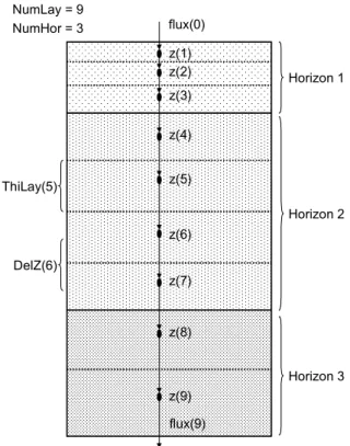
(24) page 24 of 144. RIVM report 711401 008. the gas and liquid phases, equilibrium sorption and non-equilibrium sorption, first-order transformation kinetics, uptake of pesticide by plant roots, and volatilization of pesticide at the soil surface. The core of the model is driven by a Graphical User Interface (the PEARL user interface), which is available for Windows 95/98/NT. Figure 2 shows the linkage between the individual components of PEARL. The actual linkage between the individual components is established through text and binary files (i.e. the components are loosely coupled). The basic data are stored in a relational database. The Graphical User Interface generates the input files for PEARL. SWAP input files are created by PEARL, so it is always guaranteed that both models use the same data. This is particularly important if the model is used independently from the GUI, which is the case when performing Monte Carlo simulations or inverse modeling exercises. Relevant outputs of SWAP are transferred to PEARL through a binary datafile. Summary model-outputs of PEARL are transferred to the database, where they can be retrieved and viewed by the user. Comprehensive model-outputs (e.g. vertical profiles and daily values) can be viewed with the graphical program XY, which is also driven by the PEARL user interface.. Swap core. swap.log swap.key. RunId.irr. RunID.cal. Pearl GUI. database. MeteoID.met. CropID.crp SoilID.swa. RunId.prl. Pearl core. HorID.sol RunID.hea. XY viewer. RunId.err RunId.sum. GWID.bbc MeteoId.yyy RunId.irg. RunId.out RunId.apo RunId.log. Figure 2 Dataflow diagram (DFD) for the PEARL model. Text files are double underlined.. 2.2 Vertical discretization In PEARL, soil properties are specified as a function of soil horizons. A soil horizon is assumed to have uniform chemical and physical properties. The current system allows for the definition of up to 10 soil horizons. Soil horizons are divided into numerical soil layers. Soil.

(25) RIVM report 711401 008. page 25 of 144. layers are represented by nodal points, which are situated in the center of these layers (See Figure 3, which gives an example for 9 soil layers and 3 soil horizons). The maximum number of nodal points is currently set at 500. Nodal points are characterized by a nodal height, z (m), which is negative downwards. The distance between two nodal points, ∆z (m) is calculated from: ∆z i = z i +1 − z i. (1). The maximum distance between two nodal points is given by: ∆z < 2 Ldis , L. (2). where Ldis,L (m) is the dispersion length (see section 2.5). NumLay = 9 NumHor = 3. flux(0) z(1) z(2). Horizon 1. z(3) z(4). ThiLay(5). z(5) Horizon 2 z(6). DelZ(6) z(7). z(8) Horizon 3 z(9) flux(9). Figure 3 Vertical discretization of the soil in the PEARL model.. 2.3 Hydrology 2.3.1 Soil water flow The SWAP model (Van Dam et al., 1997) uses a finite-difference method to solve the Richards equation: C ( h). ∂h ∂ é æ ∂h ö ù = ê K (h)ç + 1÷ ú − Ru , L − R d , L ∂t ∂z ë è ∂z øû. (3). where C(h) (m-1) is differential water capacity, t (d) is time, z (m) is vertical position, h (m) is soil water pressure head, K(h) (m d-1) is unsaturated hydraulic conductivity, Ru,L (m3 m-3 d-1) is volumic volume rate of root water uptake, and Rd,L (m3 m-3 d-1) is volumic volume rate of lateral discharge by drainage. SWAP can handle tabular data and analytical functions to de-.

(26) page 26 of 144. RIVM report 711401 008. scribe the soil hydraulic properties. In the PEARL context, only the analytical equations proposed by Van Genuchten (1980) are supported: θ( h ) = θ r +. θs − θr [1 + (α | h |) n ] m. and λ. [. (. K ( h) = K s S e 1 − 1 − S e. (4). ). ]. 2 1/ m m. (5). where θs (m3 m-3) is the saturated volume fraction of water, θr (m3 m-3) is the residual volume fraction of water, α (m-1) reciprocal of the air entry value, Ks (m d-1) saturated hydraulic conductivity, n (-) and λ (-) are parameters, m = 1-1/n, and Se (-) is the relative saturation, which is given by: Se =. θ − θr θs − θr. (6). 2.3.2 Potential evapotranspiration The potential evapotranspiration, ETp (m d-1) is the key variable affecting the uptake of water by plant roots and soil evaporation. SWAP uses a slightly modified version of the PenmanMonteith equation (Monteith, 1965; Van Dam et al., 1997) to calculate the potential evapotranspiration. Recent comparative studies have shown a good performance of the PenmanMonteith approach under varying climatic conditions (Jensen et al.,1990). Potential and even actual evapotranspiration calculations are possible with the Penman-Monteith equation, through the introduction of canopy and air resistance’s to water vapor diffusion. However, canopy and air resistance’s may not be available. For this reason, SWAP follows a classical two step approach, i.e. (i) the calculation of the potential evapotranspiration, using the minimum value of the canopy resistance and the actual air resistance, and (ii) the calculation of the actual evapotranspiration using a reduction function (section 2.3.4). Application of the Penman-Monteith equation requires values of the air temperature, solar radiation, wind speed and air humidity. Feddes and Lenselink (1994) proposed a methodology to use daily values of these parameters. This approach is used in SWAP. See Van Dam et al. (1997) for details. SWAP calculates three quantities with the Penman-Monteith equation: − ETw0 (m d-1) potential evapotranspiration of a wet canopy, completely covering the soil − ETp0 (m d-1) potential evapotranspiration of a dry canopy, completely covering the soil − Ep0 (m d-1) potential evaporation of a wet, bare soil. As wind speed and air humidity are not always available, PEARL can alternatively calculate the reference evapotranspiration according to Makkink (1957), which requires daily values of temperature and solar radiation only. This equation, however, has some limitations: (i) it is developed for Dutch climatological conditions, and (ii) due to the lack of a ventilation term its performance in winter conditions is relatively poor. In this case, the potential evapotranspiration rate of a dry canopy, ETp0 (m d-1) is calculated by: ET p 0 = f c ETr. (7).

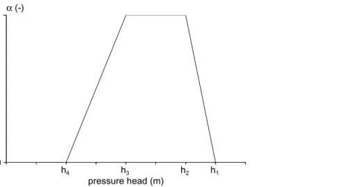
(27) RIVM report 711401 008. page 27 of 144. where fc (-) is an empirical crop factor, which depends on the crop type, and ETr (m d-1) is the reference evapotranspiration. Notice that this approach does not allow differentiation between a dry crop, a wet crop and wet soil. SWAP therefore assumes that these quantities are equal. 2.3.3 Potential transpiration and potential evaporation The potential evapotranspiration is partitioned into the potential transpiration and the potential soil evaporation (Belmans, 1983). The potential evaporation rate from a partly covered soil, Ep (m d-1) is given by E p = e − κLAI E p 0. (8). where LAI (m2 m-2) is the Leaf Area Index, κ (-) is the extinction coefficient for global solar radiation, and Ep0 (m d-1) is the potential evaporation rate of a wet bare soil. As mentioned above, Ep0 is equal to ETp0 if the Makkink equation has been used. assumes that the evaporation rate of the water intercepted by the canopy is equal to ETw0, independent of the soil cover fraction. The ratio of the daily amount of intercepted precipitation (see eqn. 14), Pi and ETw0 indicates the fraction of the day that the canopy is wet, fw (-): SWAP. fw =. Pi ETw0. (9). calculates a daily average of the potential transpiration rate, taking into account the fraction of the day that the canopy is wet (cf. Bouten, 1992): SWAP. T p = (1 − f w ) ET p 0 − E p. with T p ≥ 0. (10). where Tp (m d-1) is the potential transpiration rate in the case of a partly soil cover. 2.3.4 Uptake of water by plant roots The maximum possible root water extraction rate, integrated over the rooting depth, is equal to the potential transpiration rate, Tp (m d-1). The potential root water extraction rate at a given depth, Ru,L,p (z) (m3 m-3 d-1), is calculated from the volumic root length, Lroot (z) (m m-3) at that depth as a fraction of the integrated volumic root length (Tiktak and Bouten, 1992): Ru , L , p ( z ) =. Lroot ( z ) 0. ò Lroot ( z )dz. Tp. (11). z root. Notice that SWAP does not account for preferential uptake from layers with high relative water saturation (Herkelrath et al., 1977; Tiktak and Bouten, 1992). The actual root water extraction rate, Ru,L, is calculated using a reduction function (Figure 4, Feddes et al., 1978): Ru , L ( z ) = α w Ru , L , p ( z ). (12).

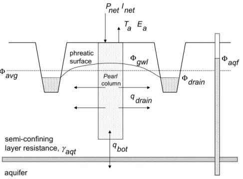
(28) page 28 of 144. 1. 0. RIVM report 711401 008. α (-). h4. h3 pressure head (m). h2. h1. Figure 4 Reduction coefficient for root water uptake, α, as a function of soil water pressure head.. 2.3.5 Evaporation of water from the soil surface To calculate the actual soil evaporation rate, the potential soil evaporation rate is first limited to the maximum flux calculated from the Darcy equation for the top nodal point, Emax. The soil evaporation flux is additionally reduced according to the method proposed by Boesten and Stroosnijder (1986), who calculated the maximum actual soil evaporation, Ea (m) during a drying cycle: å Ea = å E p. if. 2 å Ep ≤ β. å Ea = β å E p. if. 2 å Ep > β. (13). where β (m1/2) is an empirical parameter. 2.3.6 Interception of rainfall Interception of rainfall by the crop canopy is calculated from the empirical equation (Braden, 1985): é ù 1 Pi = a LAI ê1 − ú ë 1 + ( SC P ) /( aLAI ) û. (14). where Pi (m3 m-2 d-1) is intercepted precipitation, P (m3 m-2 d-1) is precipitation, SC (-) is the fraction of the soil covered by the crop, and a is an empirical parameter. In SWAP, the fraction of the soil covered by the crop is approximated by LAI/3 (Van Dam et al., 1997). 2.3.7 Bottom boundary conditions SWAP makes a distinction between the local drainage flux to ditches and drains and the seepage flux due to regional groundwater flow. The seepage flux due to regional groundwater flow is the lower boundary flux (qb), the local drainage flux is treated as a sink term (Rd,L). The following lower boundary conditions of SWAP can be used via the PEARL model: 1. Groundwater level, Φgwl (m), specified as a function of time. 2. Regional bottom flux qb (m3 m-2 d-1) specified as a function of time (Neumann condition). 3. Regional bottom flux is calculated using the hydraulic head difference between the phreatic groundwater and the groundwater in the semi-confined aquifer (pseudo two-dimensional Cauchy condition; Figure 5):.

(29) RIVM report 711401 008. qb =. page 29 of 144. Φ aqf − Φ avg. (15). γ aqt. where Фaqf (m) is hydraulic head of the semi-confined aquifer, Фavg (m) is average phreatic head, and γaqt (d) is vertical resistance of the aquitard. The average phreatic head is determined by the shape of the groundwater level in a field. The average phreatic head is calculated using the drainage base, Фd (m) and a shape-factor, βgwl: Φ avg = Φ d + β gwl (Φ gwl − Φ d ) (16) Possible values for the shape factor are 0.64 (sinusoidal), 066 (parabolic), 0.79 (elliptic) and 1.00 (no drains present). Seasonal variation of the bottom flux can be induced through a sine-wave of the hydraulic head in the semi-confined aquifer. 4. qb is calculated from an exponential flux-groundwater level relationship (Cauchy condition): qb = a g e. bg Φ avg. (17). -1. 5. 6. 7. 8.. -1. with ag (m d ) and bg (m ) as empirical coefficients. Pressure head of the bottom soil layer specified as a function of time (Dirichlet condition). Zero flux at bottom of soil profile: qb = 0 (special case of Neumann condition). Free drainage of soil profile, in which case unit gradient is assumed at the lower boundary: qb = -KNumLay (special case of Neumann condition). Lysimeter boundary condition: Outflow only occurs if the pressure head of the bottom soil layer is above zero (special case of Neumann condition).. 2.3.8 Lateral discharge of soil water Lateral discharge rates can be calculated for a maximum number of five local drainage systems (e.g. drainage tiles and field-ditches). PEARL uses the following equation to calculate the flux to drainage system k: qd ,k =. Φ avg − Φ d ,k γ d ,k. (18). where qd,k (m3 m-2 d-1) is the flux of water to local drainage system k, Φd,k (m) is hydraulic head of drainage system k, and γd,k (d) is drainage resistance. In order to distribute the discharge rates over the soil layers, first a discharge layer is determined by considering a traveltime distribution. The most important assumption in this computational procedure is that lateral discharge occurs to parallel, equidistant water courses (distance Lk (m)). See chapter 10.1 in Van Dam et al. (1997) for details. Within this discharge layer, the lateral drainage from soil layer i to local drainage system k, Rd,L,k,i, is calculated with the equation: R d , L , k ,i =. qd ,k. K s ,i ∆z i. ∆z i å ( K s ,i ∆z i ). (19). The total lateral drainage is calculated by summing the lateral drainage for all local drainage systems..

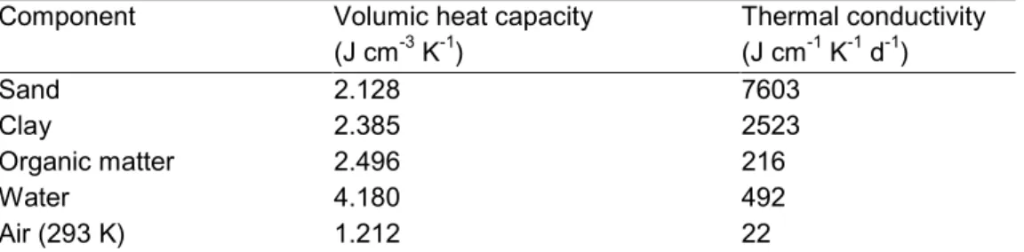
(30) page 30 of 144. RIVM report 711401 008. P I net net T E a a phreatic surface. Φ. avg. Φ Pearl column. Φ q. semi-confining layer resistance, γ aqt. q. Φ. gwl. aqf. drain. drain. bot. aquifer. Figure 5 Pseudo two-dimensional Cauchy lower boundary condition, in case of drainage to ditches (Van Dam et al., 1997).. 2.4 Heat flow The model SWAP (Van Dam et al., 1997) calculates conductive transport of heat in soil: ∂ChT ∂ é ∂T ù = êλ ú ∂t ∂z ë ∂z û. (20). where Ch (J m-3 K-1) is the volumic heat capacity, T (K) is temperature, and λ (J m-1 d-1 K-1) is the effective heat conductivity. The volumic heat capacity is calculated as the weighted mean of the heat capacities of the individual soil components (De Vries, 1963): C h = θ sand C sand + θ clay C clay + θ om C om + θC w + εC a. (21). where θsand, θclay, θom and θ (m3 m-3) are the volume fractions of sand, clay, organic matter and water, ε (m3 m-3) is the air-filled porosity, and Csand, Cclay, Com, Cw and Ca (J m-3 K-1) are the volumic heat capacities of the individual components. Table 1 gives an overview of the volumic heat capacity for the individual soil components. The volume fractions of sand, clay and organic matter are calculated from the mass percentages of sand, clay and organic matter, which are input to the model. The thermal conductivity is calculated according to the procedure described by Ashby et al. (1996), which accounts for both soil composition and soil geometry..

(31) RIVM report 711401 008. page 31 of 144. Table 1 Volumic heat capacity and thermal conductivity of the individual soil components (after Van Dam et al., 1997). Component Sand Clay Organic matter Water Air (293 K). Volumic heat capacity -3 -1 (J cm K ) 2.128 2.385 2.496 4.180 1.212. Thermal conductivity -1 -1 -1 (J cm K d ) 7603 2523 216 492 22. The upper boundary condition for the soil heat-flow model is the daily average air temperature, Tair (K); the lower boundary condition is a zero-flux boundary condition. The heat flow equation is solved using a numerical method.. 2.5 Pesticide fate 2.5.1 Pesticide application Various factors affect the fraction of the dosage that is introduced into the soil system. During spraying, a fraction of the nominal dosage may be intercepted by the crop canopy. A part of the nominal dosage may drift from the field to adjacent ditches and fields. Another part may dissipate at the soil surface by processes like film volatilization and photochemical transformation. In PEARL, the user can choose from two general methods to describe the dosage introduced into the system: 1. Pesticide losses above the soil system are estimated beforehand, and the net load is introduced directly into the soil system. 2. The processes at the soil surface and plant surface are simulated in a simplified way. 2.5.2 Canopy processes When a pesticide is sprayed on a field grown with plants, the nominal dosage has to be distributed over the plant canopy and the soil surface: Ad , p = SC Ad , f. (22). Ad ,s = (1 − SC ) Ad , f. (23). and where Ad,f (kg m-2) is the areic mass of pesticide applied to the field, Ad,p (kg m-2) is the areic mass of pesticide applied to the crop canopy, Ad,s (kg m-2) is the areic mass of pesticide deposited on the soil, and SC (-) is the fraction of the soil surface covered by the crop. All areic masses are expressed per m2 field surface. Methods are being developed for more targeted spraying on plants or on the soil surface, so the soil cover fraction may not be appropriate. In this particular case, the fraction of the dosage that is deposited onto the crop canopy can be introduced by the user. The following processes are described at the plant surface: (i) volatilization into the air, (ii) penetration into the plant, (iii) transformation at the plant surface, and (iv) wash-off via rainfall. The first three processes are described by first-order kinetics:.

(32) page 32 of 144. RIVM report 711401 008. Rdsp = k v , p Ap + k p , p Ap + k t , p Ap. (24). where Rdsp (kg m-2 d-1) is the areic mass rate of dissipation of pesticide at the plant surface, kv,p (d-1) is rate coefficient for volatilization, kp,p (d-1) is rate coefficient for penetration, kt,p (d-1) is rate coefficient for transformation at the plant surface, and Ap (kg m-2) is areic mass of pesticide at the crop canopy. Alternatively, the user can introduce an overall dissipation rate coefficient, kdsp (d-1) for the three processes. The areic mass rate of pesticide wash-off is taken proportional to the canopy drip flux: R w, p = w p ( SC P − Pi ) A p. (25). where Rw,p (kg m-2 d-1) is the areic mass rate of pesticide wash-off from the crop canopy, wp (m-1) is an empirical wash-off factor, P (m d-1) is precipitation, and Pi (m d-1) is intercepted water. The following mass balance applies for the crop canopy: ∂A p ∂t. = − Rw, p − Rdsp. (26). 2.5.3 Mass balance equations Pesticide can be found in the equilibrium domain and in the non-equilibrium domain of the soil system (Figure 6), so two mass balances apply: ∂ceq* ∂t. = − Rs −. ∂J p , L ∂z. −. ∂J p , g ∂z. − Rt + R f − Ru − Rd. (27). and ∂cne* = Rs ∂t. (28). Here, c*eq (kg m-3) is the pesticide concentration in the equilibrium domain of the soil system, c*ne (kg m-3) is the pesticide concentration in the non-equilibrium domain of the soil system, Rs (kg m-3 d-1) is the volumic mass rate of pesticide sorption, Jp,L (kg m-2 d-1) is the mass flux of pesticide in the liquid phase, Jp,g (kg m-2 d-1) is the mass flux of pesticide in the gas phase, Rt (kg m-3 d-1) is the transformation rate, Rf (kg m-3 d-1) is the formation rate, Ru (kg m-3 d-1) is the rate of pesticide uptake by plant roots, and Rd (kg m-3 d-1) is the lateral discharge rate of pesticides. 2.5.4 Transport in the liquid phase Transport of the pesticide in the liquid phase of the soil is described by an equation including convection, dispersion and diffusion: J p , L = qc L − Ddis , L. ∂c L ∂c − Ddif , L L ∂z ∂z. (29). where Jp,L (kg m-2 d-1) is the mass flux of pesticide in the liquid phase, q (m3 m-2 d-1) is the soil water flux, Ddis,L (m2 d-1) is coefficient of pesticide dispersion in the liquid phase, z (m) is vertical position, and Ddif,L (m2 d-1) is the coefficient of pesticide diffusion in the liquid phase. The dispersion coefficient is taken to be proportional to the soil water flux: Ddis , L = Ldis , L q. (30).

(33) RIVM report 711401 008. page 33 of 144. with Ldis,L (m) as the dispersion length. The diffusion of pesticide in the liquid phase is described by Fick’s law. The coefficient for diffusion of pesticide in the liquid phase is calculated by: Ddif , L = ζ L Dw. (31). where ζL (-) is the relative diffusion coefficient in the liquid phase, and Dw (m2 d-1) is the coefficient of pesticide diffusion in pure water.. Equilibrium domain of the soil system Liquid phase c L. Solid phase X eq. fast processes Gas phase c g. slow processes. X* ne. c* eq. Non-equilibrium domain of the soil system. Figure 6 Diagram of equilibrium and non-equilibrium domains of the soil system.. The relative diffusion coefficient is a function of the volume fraction of liquid. PEARL offers three methods do describe this function. By default, the function proposed by Millington and Quirk (1960) is used: ζL = θ 3. a M ,L. b. (32). θ s M ,L. -3. 3. -3. where θ (m m ) is the volume fraction of liquid, θs (m m ) is the volume fraction of liquid at saturation, and aM,L (-) and bM,L (-) are empirical parameters. The second type of equation is the one used by Currie (1960): ζ L = aC , L θ. bC , L. (33). where aC,L (-) and bC,L (-) are empirical coefficients. The third equation is suggested by Troeh et al. (1982). In this approach, diffusion in the liquid phase is taken to be zero in a range of (low) volume fractions of water. In this range, the water-filled pores are assumed to be discontinuous: æ θ − aT , L ö ÷ ì ç ζ L = í ç 1 − aT , L ÷ è ø î 0. bT , L. if. θ > aT , L. if. θ ≤ aT , L. (34).

(34) page 34 of 144. RIVM report 711401 008. where aT,L (m3 m-3) is the volume fraction of water at the air-entry point, and bT,L (-) is an empirical parameter. The value of the diffusion coefficient in water is temperature dependent, mainly because the viscosity of water depends on the temperature. In PEARL, the theoretically derived StokesEinstein equation (Tucker and Nelken, 1982) is approximated by: Dw = 1 + 0.02571(T − Tr )Dw,r. (35). where T (K) is temperature, Tr (K) is reference temperature, and Dw,r (m2 d-1) is the diffusion coefficient in water at reference temperature. See Leistra et al. (2000) for details. 2.5.5 Transport in the gas phase Transport of pesticide in the gas phase is described by Fick’s law: J p , g = − Ddif , g. ∂c g ∂z. (36). where Jp,g (kg m-2 d-1) is mass flux of pesticide in the gas phase, and Ddif,g (m2 d-1) is coefficient of pesticide diffusion in the gas phase. The coefficient for diffusion of pesticide in the gas phase is calculated by: Ddif , g = ζ g Da. (37). where ζg (-) is the relative diffusion coefficient in the gas phase, and Da (m2 d-1) is the coefficient of pesticide diffusion in air. The relation between Da and temperature is described by: æT D a = çç è Tr. ö ÷÷ ø. 1.75. Da , r. (38). where Da,r (m2 d-1) is the diffusion coefficient in air at reference temperature. The relative diffusion coefficient is a function of the volume fraction of the gas phase. It is calculated analogous to the relative diffusion coefficient in the liquid phase (eqn. 32-34). 2.5.6 Initial and boundary conditions The initial condition for the model is defined by profiles of the concentration of pesticide in the equilibrium domain of the soil system, c*eq (kg m-3), and in the non-equilibrium domain of the soil system, c*ne (kg m-3). It is further assumed that at the start of the simulation the areic mass of pesticide at the plant surface, Ap, is zero. The boundary condition at the soil surface is a flux boundary condition. The user can enter deposition fluxes of pesticide as a function of time. Pesticides entering the system by deposition are subject to canopy processes. The user can also specify the concentration of pesticide in irrigation water, in which case the user has to choose between surface irrigation (i.e. application of irrigation water directly to the soil system) and sprinkler irrigation (application to the crop canopy). At the lower boundary of the soil system, dispersive and diffusive fluxes of pesticide are assumed to be zero. In the case of infiltration of water from a deep aquifer, the pesticide concentration is set to zero..

(35) RIVM report 711401 008. page 35 of 144. Diffusion of pesticide vapor in the gas phase of the soil is included in the model, which implies that a description of pesticide volatilization at the soil surface is required. In the current model version, the diffusion of vapor through the soil and a laminar air-boundary layer are the limiting factors for volatilization (cf. Jury et al., 1990): J p ,v =. cg. (39). rs ,v + ra ,v. where Jp,v (kg m-2 d-1) is the mass flux of pesticide volatilization, cg (kg m-3) is concentration of pesticide in the gas phase of the top layer, rs,v (d m-1) is resistance of the soil boundary layer, and ra,v (d m-1) is resistance of the air boundary layer. The resistance’s of the boundary layers are calculated by: rs ,v =. ds Ddif , g. and. ra ,v =. da Da. (40). where ds (m) is thickness of soil boundary layer, Ddif,g (m2 d-1) is the coefficient for diffusion of pesticide in the gas phase of the soil system, da (m) is the thickness of the laminar airboundary layer, and Da (m2 d-1) is coefficient for diffusion of pesticide in air. It should be noted that the current description of pesticide volatilization is subject to considerable uncertainty, particularly for surface-applied pesticides where initial volatilization is hardly limited by the soil boundary layer. For this reason, at present research aimed at improving the submodel for pesticide volatilization is being carried out. See Leistra et al. (2000) for further considerations. 2.5.7 Partitioning over the three soil phases The sorption of pesticide on the soil solid phase is described with a Freundlich equation. Both equilibrium and non-equilibrium (kinetic) sorption are considered. Equilibrium sorption is described by the equation: X eq. æ c = K F ,eq c L ,r ç L çc è L,r. ö ÷ ÷ ø. N. (41). in which Xeq (kg kg-1) is pesticide content in the equilibrium sorption phase, KF,eq (m3 kg-1) is Freundlich coefficient for the equilibrium-sorption phase, cL (kg m-3) is concentration in the liquid phase, cL,r (kg m-3) is reference concentration in the liquid phase and N is the Freundlich exponent. Notice that a particular type of Freundlich equation is used in the model, by introducing the reference concentration. The advantage of this type of equation is that the unit of the Freundlich coefficient becomes independent of the exponent. The Freundlich coefficient may depend on various soil properties, such as organic matter content, oxide content and pH. For most pesticides, the following equation is appropriate: K F ,eq = mom K om ,eq. (42). where mom (kg kg-1) is mass content of organic matter in soil and Kom,eq (m3 kg-1) is the coefficient of equilibrium sorption on organic matter..

(36) page 36 of 144. PEARL. RIVM report 711401 008. contains a description of the sorption of weak acids, which is pH dependent: K om.eq,ac + K om ,eq ,ba K F,eq = mom. 1+. M ba pH- pKa-∆pH 10 M ac. M ba pH - pKa -∆pH 10 M ac. (43). where Kom,eq,ac (m3 kg-1) is the coefficient for sorption on organic matter under acidic conditions, Kom,eq,ba (m3 kg-1) is the coefficient for sorption on organic matter under basic conditions, M (kg mol-1) is molar mass, pKa is the negative logarithm of the dissociation constant, and ∆pH is a pH correction factor. See Leistra et al. (2000) for the derivation of this equation. The sorption of some specific pesticides cannot be described with the organic matter equilibrium constant. This is particularly true for those pesticides that sorb preferentially on clay and oxides. In this case, the user should specify the Freundlich coefficient of the topsoil and a depth-effect factor: K F ,eq = f d , s K F ,eq ,r. (44). where KF,eq,r (m3 kg-1) is the Freundlich coefficient in the topsoil, and fd,s (-) is an empirical depth-effect factor. Pesticide sorption to the non-equilibrium phase is described by a first-order rate equation: é æc Rs = ρ b k d ê f K ,ne K F ,eq c L ,r ç L çc ê è L,r ë. N ù ö ÷ − X ne ú ÷ ú ø û. (45). where Rs (kg m-3 d-1) is rate of sorption in the non-equilibrium domain of the soil system, ρb (kg m-3) is the dry bulk density of the soil, Xne (kg kg-1) is pesticide content at non-equilibrium sorption sites, kd (d-1) is desorption rate coefficient, and fK,ne (-) is factor describing the ratio KF,ne/KF,eq, with KF,ne (m3 kg-1) as the Freundlich coefficient for the non-equilibrium sorption phase. See Leistra et al. (2000) for a discussion of the theoretical background of this equation. The partitioning of the pesticide between the gas phase and the liquid phase is described by Henry’s law: c g = K H cL. (46). in which cg (kg m-3) is the concentration of pesticide in the gas phase and KH (m3 m-3) is the Henry coefficient, which is calculated by: KH =. pv ,s M S w RT. (47). where pv,s (Pa) is the saturated vapor pressure, M (kg mol-1) is molar mass, Sw (kg m-3) is solubility in water, R (J mol-1 K-1) is the molar gas constant, and T (K) is the temperature. PEARL describes the temperature dependence of both pv,s, which requires the molar enthalpy of vaporization, ∆Hv (J mol-1), and Sw, which requires the molar enthalpy of dissolution, ∆Hd (J mol-1):.

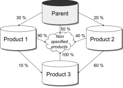
(37) RIVM report 711401 008. page 37 of 144. é − ∆H v pv , s = pv , s ,r exp ê êë R. æ 1 1 öù çç − ÷÷ú è T Tr øúû. (48). and é − ∆H d S w = S w,r exp ê êë R. æ 1 1 öù çç − ÷÷ú è T Tr øúû. (49). Here, pv,s,r (Pa) is the saturated vapor pressure at reference temperature Tr (K) and Sw,r (kg m-3) is the pesticide solubility in water at reference temperature. The total concentration of pesticide in the equilibrium domain of the soil system (kg m-3) is given by: ceq* = εc g + θc L + ρ b X eq. (50). where ε (m3 m-3) is volume fraction of the gas phase, cg (kg m-3) is concentration of pesticide in the gas phase, θ (m3 m-3) is volume fraction of the liquid phase, cL (kg m-3) is concentration of pesticide in the liquid phase, ρb (kg m-3) dry bulk density of the soil, and Xeq (kg kg-1) is pesticide mass content in the equilibrium phase. The total concentration of pesticide in the non-equilibrium phase (kg m-3) is given by: cne* = ρ b X ne. (51). with Xne (kg kg-1) as the pesticide mass content in the non-equilibrium phase. 2.5.8 Transformation of pesticide in soil Transformation of pesticides may lead to reaction products (daughters) that may show a certain degree of persistence and mobility in soils. For this reason, the formation and behavior of the most important daughters is included in PEARL. The first step in the definition of the reaction scheme is to set up the list of compounds that will be considered. The second step is the definition of the pathways of pesticide transformation. Consider the example shown in Figure 7. The reaction scheme presented in Figure 7 can be represented in matrix notation as shown in Table 2. This example shows that a compound may transform into various products and that they may be formed from more than one precursor compound..

(38) page 38 of 144. RIVM report 711401 008. Parent. 30 %. 20 %. 50 %. Product 1. 90 %. Non specified products. 40 %. Product 2. 100 % 10 %. 60 %. Product 3. Figure 7 Example of a reaction scheme of a pesticide. Table 2 Example of a matrix, which represents the reactions between one parent and three reaction products. A value of zero indicates no interaction.. Parent Product 1 Product 2 Product 3. Parent 0.0 0.0 0.0 0.0. Product 1 0.3 0.0 0.0 0.0. Product 2 0.2 0.0 0.0 0.0. Product 3 0.0 0.1 0.6 0.0. In PEARL 1.1, the rate of transformation of a precursor (parent) is described by a first-order rate equation: Rt , par = k t , par ceq* , par. (52). in which Rt,par (kg m-3 d-1) is the rate of transformation of the parent pesticide, kt,par (d-1) is the transformation rate coefficient, and c*eq,par (kg m-3) is the concentration of the parent pesticide in the equilibrium domain of the soil. Notice that pesticide residing in the non-equilibrium domain is not transformed. The rate of formation of a daughter from a parent, Rf,par,dau (kg m-3 d-1), is subsequently calculated by: R f , par ,dau = χ par ,dau. M dau Rt , par M par. (53). where χ par,daugher (-) is the molar fraction of parent transformed to daughter, and M (kg mol-1) is the molar mass. The rate of pesticide transformation in soil depends on the temperature, soil moisture content and the depth in soil: k t = f t f m f d k t ,r. (54).

(39) RIVM report 711401 008. page 39 of 144. where ft (-) is the factor for the effect of temperature, fm (-) is the factor for the effect of soil moisture, fd (-) is the factor for the effect of depth in soil, and kt,r (d-1) is the rate coefficient at reference conditions, which is calculated from: k t ,r =. ln(2) DT50 ,r. (55). where DT50,r (d) is the half-life of the pesticide in the well-moistened plough layer at reference temperature. The effect of temperature on the pesticide transformation rate is described by the Arrhenius equation: é − Ea f t = exp ê êë R. æ 1 1 öù çç − ÷÷ ú è T Tr ø úû. (56). where Ea (J mol-1) is molar activation energy, R (J mol-1 K-1) is the molar gas constant, and T (K) is temperature. The Arrhenius equation is assumed to be valid from 5 to 35 oC. Above 35 oC, the factor for the effect of temperature is kept constant. At temperatures below zero, the factor for the effect of temperature is set to zero (Jarvis, 1994). This implies that no pesticide transformation is simulated in frozen soil. The equation for the effect of soil water on transformation reads (Walker, 1974): é æ θ f m = min ê1, ç ê çè θ fc ë. ö ÷ ÷ ø. B. ù ú ú û. (57). where θ (m3 m-3) is volume fraction of soil water, B (-) is empirical factor for the effect of soil moisture, and the suffix fc refers to field capacity. The effect of depth on the rate of transformation in soil is described by a tabular relationship. 2.5.9 Pesticide uptake The uptake of pesticide by plant roots is described by the equation: Ru = Ru , L f u c L -3. -1. (58) 3. -3. -1. where Ru (kg m d ) is volumic mass rate of pesticide uptake, Ru,L (m m d ) is volumic volume rate of water uptake, and fu (-) is an empirical transpiration stream concentration factor. 2.5.10 Lateral discharge of pesticides The rate of water discharged by the tile-drainage system is calculated by the hydrological submodel (eqn. (19)). The lateral discharge of pesticides is taken proportional to the water fluxes discharged by the tile-drainage system: R d = Rd , L c L. (59). where Rd (kg m-3 d-1) is volumic mass rate of pesticide discharge, and Rd,L (m3 m-3 d-1) is volumic volume rate of water discharge. Equation 59 implies that it is assumed that concentration gradients in the lateral direction are negligible (i.e. no diffusion/dispersion)..


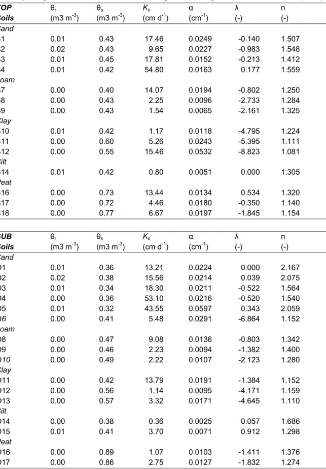
(41) RIVM report 711401 008. 3. page 41 of 144. Model parameterization. In a ring-test of 9 European pesticide leaching models (Vanclooster et al.¸ 2000), subjectivity in the derivation of model inputs was the major source of differences between model results (Tiktak, 2000; Boesten, 2000). An important recommendation was to provide to model-users with strict guidelines and additional tools for deriving model inputs. We therefore included this chapter, which gives an overview of methods to derive the most important model inputs. In the pesticide registration procedure (e.g. Linders et al., 1994), several stages can be distinguished. In first-tier assessments, the model is used to get a first indication of the leaching potential of a pesticide. To minimize user subjectivity during this stage, the model is used in combination with standardized scenario’s (FOCUS, 2000). These scenario’s are supported by PEARL (chapter 5). The following steps should be followed: 1. Specification of pesticide properties, including the half-life at reference temperature (DT50,r, see section 3.2.9), the coefficient for sorption on organic matter (Kom,eq, see section 3.2.6), the saturated vapor pressure at reference temperature (pv,s,r, see section 3.2.8), and the solubility in water (Sw,r, see section 3.2.8). 2. Selection of crop type. 3. Selection of one or more locations. 4. Selection of application schedule (annual, biennial, triennial) and the actual application dates. By selecting a combination of location, crop type and application schedule most model-inputs are fixed. During the second and higher tiers of the registration procedure, field studies and lysimeter experiments may become important. During this stage, the model should preferably be used in combination with on-site measured data. Guidelines for model parameterization follow below.. 3.1 Hydrology 3.1.1 Soil water flow Soil water transport is described with the Richards equation (eqn. 3). The soil hydraulic properties are described with analytical functions (eqn. 4 and 5). Parameter values can be obtained by fitting experimentally derived retention data to eqn. 4 and 5, using the RETC program (Van Genuchten et al., 1991). See Van Dam et al. (1997) for an overview of experimental procedures to obtain the soil hydraulic characteristics. Parameter values for the Van Genuchten (1980) analytical functions can be found in a number of international and.

(42) page 42 of 144. RIVM report 711401 008. Table 3 Dataset of soil hydraulic functions (Wösten et al., 1994), based on Dutch texture classes (Table 4). The function are described with the analytical model of Mualem-Van Genuchten (1980). TOP Soils Sand B1 B2 B3 B4 Loam B7 B8 B9 Clay B10 B11 B12 Silt B14 Peat B16 B17 B18 SUB Soils Sand O1 O2 O3 O4 O5 O6 Loam O8 O9 O10 Clay O11 O12 O13 Silt O14 O15 Peat O16 O17. θr -3 (m3 m ). θs -3 (m3 m ). Ks -1 (cm d ). α -1 (cm ). λ (-). n (-). 0.01 0.02 0.01 0.01. 0.43 0.43 0.45 0.42. 17.46 9.65 17.81 54.80. 0.0249 0.0227 0.0152 0.0163. -0.140 -0.983 -0.213 0.177. 1.507 1.548 1.412 1.559. 0.00 0.00 0.00. 0.40 0.43 0.43. 14.07 2.25 1.54. 0.0194 0.0096 0.0065. -0.802 -2.733 -2.161. 1.250 1.284 1.325. 0.01 0.00 0.00. 0.42 0.60 0.55. 1.17 5.26 15.46. 0.0118 0.0243 0.0532. -4.795 -5.395 -8.823. 1.224 1.111 1.081. 0.01. 0.42. 0.80. 0.0051. 0.000. 1.305. 0.00 0.00 0.00. 0.73 0.72 0.77. 13.44 4.46 6.67. 0.0134 0.0180 0.0197. 0.534 -0.350 -1.845. 1.320 1.140 1.154. Ks -1 (cm d ). α -1 (cm ). θr -3 (m3 m ). θs -3 (m3 m ). λ (-). n (-). 0.01 0.02 0.01 0.00 0.01 0.00. 0.36 0.38 0.34 0.36 0.32 0.41. 13.21 15.56 18.30 53.10 43.55 5.48. 0.0224 0.0214 0.0211 0.0216 0.0597 0.0291. 0.000 0.039 -0.522 -0.520 0.343 -6.864. 2.167 2.075 1.564 1.540 2.059 1.152. 0.00 0.00 0.00. 0.47 0.46 0.49. 9.08 2.23 2.22. 0.0136 0.0094 0.0107. -0.803 -1.382 -2.123. 1.342 1.400 1.280. 0.00 0.00 0.00. 0.42 0.56 0.57. 13.79 1.14 3.32. 0.0191 0.0095 0.0171. -1.384 -4.171 -4.645. 1.152 1.159 1.110. 0.00 0.01. 0.38 0.41. 0.36 3.70. 0.0025 0.0071. 0.057 0.912. 1.686 1.298. 0.00 0.00. 0.89 0.86. 1.07 2.75. 0.0103 0.0127. -1.411 -1.832. 1.376 1.274.

No results found