Indirecte baten van klimaatbeleid

(1)

Netherlands Environmental Assessment Agency, February 2009

Co-benefits of

climate policy

Global climate policy will reduce outdoor air

pollution

A stringent global climate policy will lead to considerable improvements in local air quality and consequently improves human health. Measures to reduce emissions of greenhouse gases to 50% of 2005 levels, by 2050, can reduce the number of premature deaths from the chronic exposure to air pollution by 20 to 40%. Climate policy will already generate air quality improvements in the OECD countries (particularly in the USA) in the mid-term, whereas in developing countries these benefits will only in the longer run show to be significant. This is the main message of this report that was carried out for the OECD.

Background Studies

C

(2)

(3)

(4)

(5)

PBL Report no. 500116005

Co-benefits of climate policy

(6)

PBL Report no. 500116005, Februari, 2009

J.C. Bollen, C.J. Brink, H.C. Eerens, A.J.G. Manders Contact:

Johannes Bollen PBL/MNP/KMD johannes.bollen@pbl.nl

Parts of this publication may be reproduced, on condition of acknowledgement: ‘Netherlands Environmental Assessment Agency, the title of the publication and year of publication.’

Netherlands Environmental Assessment Agency (PBL) PO Box 303 3720 AH Bilthoven The Netherlands T: +31 (0)30 274 2745 F: +31 (0)30 274 4479 E: info@pbl.nl www.pbl.nl/en

(7)

About this report

About this report

Global climate policy will reduce outdoor air pollution

A stringent global climate policy will lead to considerable improvements in local air quality and consequently improves health. Measures to reduce emissions of greenhouse gases to 50% of 2005 levels, by 2050, can reduce the number of premature deaths from the chronic exposure to air pollution by 20 to 40%. Climate policy will already generate air quality improvements in the oecd countries (particularly in the us) in the mid-term, whereas in developing countries these benefits will only in the longer run show to be significant. This is the main message of a report published by the Netherlands Environmental Assessment Agency (pbl), titled ‘Co-benefits of climate policy’ that was carried out for the oecd.

Synergy between air pollution and climate policies

Combustion of fossil energy leads to climate change and air pollution. The oecd, therefore, posed the question if a global climate policy could bring additional benefits by reducing outdoor air pollution, with the associated positive effects on public health. The potential additional benefits can be an extra incentive for countries to participate in a future climate agreement. The study by the Netherlands Environmental Assessment Agency (pbl) indicates that there is indeed a synergy between these policy areas. An integrated strategy tackling climate change and air pollution will reduce the policy costs and generate a net welfare benefit at the global level. The co-benefits of uniform carbon prices around the world will in the medium term become visible in the rich oecd countries, and in the longer run in non-oecd countries. In these latter countries, however, the costs of such a uniform global climate policy would initially outweigh the benefits of better air quality. Moreover, the pbl report reveals that in developing countries these air quality improvements can be achieved more cheaply by pursuing a directed air quality policy.

Insufficient incentive

Although the indirect benefits of climate policy – improved air quality and public health – could be an additional incentive for countries to participate in a future climate convention, they are too small to outweigh the costs of climate policy. For example, in 2050, the costs of such a climate policy in China – under which greenhouse gas emissions are 80% lower than the baseline trend without that policy – will amount to 6.5% of the country’s gdp. Meanwhile, the benefits will be equivalent to 4.5% of gdp. However, these benefits could also be achieved through a more targeted air quality policy. In China, such a targeted air quality policy could achieve the same air quality improvements by 2050, at a cost of 1.8% of gdp.

Stringent air pollution policy This study also shows that a stringent air quality policy can lead to a reduction in emissions of greenhouse gases. For example, if China pursues a stringent air policy to reduce the number of premature deaths from chronic exposure to outdoor air pollution by 70%, by 2050 (compared with a baseline trend without policy), this policy will lower gdp in 2050 by 7%. The air quality benefits would be equivalent to 7.5% of gdp, while greenhouse gas emissions would be 40% lower.

(8)

(9)

1 Typografie

Rapport in het kort

Mondiaal klimaatbeleid leidt tot verbetering van luchtkwaliteit

Streng mondiaal klimaatbeleid leidt tot een forse verbetering van de lokale luchtkwaliteit en daarmee tot minder gezondheidsverlies. Maatregelen om in 2050 de wereldwijde uitstoot van broeikasgassen te verlagen tot 50% van het niveau in 2005 kunnen de vroegtijdige sterfte door chronische blootstelling aan luchtvervuiling verminderen met 20-40%. De verbetering van de luchtkwaliteit als gevolg van klimaatbeleid zal sneller zichtbaar zijn in de OESO-landen (vooral in de VS) en pas later in ontwikkelingslanden. Dat blijkt uit deze studie, die is uitgevoerd in opdracht van de OESO.

Synergie tussen luchtvervuiling en klimaatverandering

De verbranding van fossiele energie leidt tot klimaatverandering én luchtvervuiling. De OESO veronderstelt daarom dat een mondiaal klimaatbeleid bijkomende voordelen zou kunnen hebben voor de vermindering van luchtvervuiling en de daarmee gepaard gaande positieve gevolgen voor de gezondheid. Die mogelijke bijkomende voordelen kunnen landen een extra prikkel geven om mee te doen aan een toekomstig klimaatverdrag. Uit de studie van het Planbureau voor de Leefomgeving blijkt dat er inderdaad synergie bestaat tussen de beleidsterreinen. Een geïntegreerde aanpak van klimaatverandering en luchtvervuiling vermindert de kosten van beleid, en leidt tot een netto welvaartswinst op mondiaal niveau.

De voordelen van wereldwijde uniforme klimaatbeprijzing zullen op de middellange termijn al zichtbaar zijn in de rijke, OESO-landen en op de wat langere termijn ook buiten de OESO. In ontwikkelingslanden echter wegen de kosten van zo’n wereldwijd uniform klimaatbeleid vooralsnog niet op tegen de baten van luchtkwaliteit. Dit rapport laat bovendien zien dat in deze landen de luchtkwaliteit goedkoper verbeterd kan worden door gericht streng luchtbeleid. Prikkel onvoldoende

Ofschoon de indirecte baten van klimaatbeleid – namelijk een verbetering van de luchtkwali-teit en gezondheid – een extra prikkel zouden kunnen zijn voor landen om mee te doen aan een toekomstig klimaatverdrag, zijn deze te klein om de kosten van het klimaatbeleid te overtreffen. In China zullen bijvoorbeeld de kosten van het klimaatbeleid in 2050 – leidend tot een 80% vermindering van broeikasgassen ten opzichte van het basispad zonder beleid - gelijk zijn aan 6,5% van het BBP. Terwijl de luchtbaten dan gelijk zullen zijn aan 4,5% van het BBP. Wel moet aangetekend worden dat deze baten via een meer gericht luchtbeleid ook gerealiseerd kunnen worden. In China kan in 2050 met 1,8% van het BBP dezelfde luchtbaten worden behaald door gericht luchtbeleid.

Streng luchtbeleid

Deze studie laat ook zien dat streng luchtbeleid op zijn beurt kan leiden tot vermindering van de uitstoot broeikasgassen. Als in China bijvoorbeeld zo’n streng luchtbeleid erop gericht is om in 2050 70% van de vroegtijdige sterfgevallen door luchtvervuiling te vermijden (ten opzichte van een basispad zonder beleid), dan zal dit beleid het BBP in 2050 met 7% verlagen. De luchtbaten zijn in dat geval gelijk aan 7,5% van het BBP, terwijl de uitstoot van broeikasgassen in dat geval 40% lager uitvallen.

Trefwoorden: klimaatverandering, luchtvervuiling, integratie, schadekosten, kosten-baten analyse

(10)

(11)

Contents

Summary

Policy perspectives on Climate Change and Air Pollution

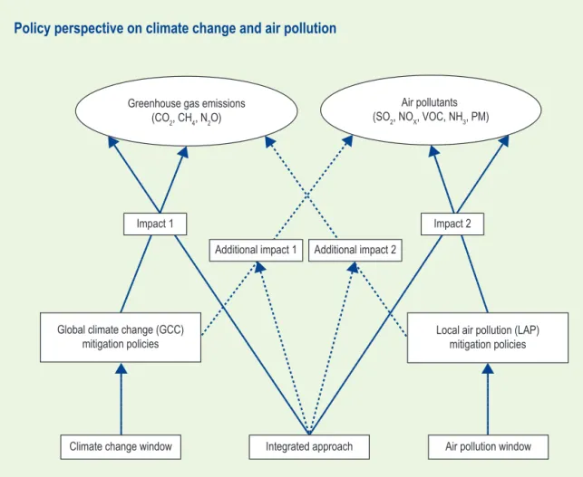
This report investigates the consequences of the interrelationship between global climate change (GCC) and local air pollution (LAP). The major connection between these environmental prob-lems is the combustion of fossil fuels. As a consequence, policies aiming to mitigate one of these environmental problems potentially have large effects on the other. For example, climate policy may reduce the demand for coal in the electricity sector, which lowers emissions that contribute to local air pollution. 1)_{From an efficiency point of view, it is important to take into} account these co-effects when deciding on appropriate policy actions in response to one of these problems. Also for a country’s decision to participate in an international environmental agree-ment (for example on climate change), the incentive not only depends on the direct costs and benefits of this policy strategy, but also on the co-effects of the policy under consideration. The present study investigates the interrelations between policies for climate change and poli-cies for local air pollution from three different perspectives or windows (see Figure 1, based on Bollen et al., 2009):

i. Climate change window: policies primarily aiming at the mitigation of global climate change not only reduce emissions of greenhouse gases (Impact 1), but also reduce emissions of air pollutants (Additional impact 1), which yields co-benefits in terms of reduced local air pollution;

ii. Air pollution window: policies primarily aiming at the mitigation of local air pollution not only reduce emissions of air pollutants (Impact 2), but also reduce emissions of greenhouse gases (Additional impact 2), yielding co-benefits in terms of reduced global climate change; iii. Integrated approach: policies are simultaneously aiming at the mitigation of global climate

change (Impact 1 + Additional impact 2) and local air pollution (Impact 2 + Additional impact 1), yielding an optimised combination of reductions in emissions of greenhouse gases and air pollutants.

In this report, the costs and benefits (including the co-benefits) are estimated for different environmental policies. In the climate change window and the air pollution window, co-benefits are calculated in two alternative ways. First, co-benefits are calculated as the monetary value of the avoided disutility (compared with the Business-As-Usual (BAU) scenario) associated with the damage from local air pollution (premature deaths) and global climate change (tempera-ture rise), respectively. Second, co-benefits are calculated as the avoided costs and benefits of alternative policy packages that would yield the same co-benefit (i.e. reduction in premature deaths and greenhouse gas emissions, respectively) at minimum cost. The reason to do so is that, although co-benefits calculated in the first way may be substantial, if these benefits can be achieved at lower cost by an alternative policy package (i.e. co-benefits calculated in the second way are lower than calculated in the first way), this is a more appropriate figure to evaluate whether co-benefits form an incentive to participate in an international agreement. Indeed, for example in the climate window, the number of premature deaths prevented through the climate policy can also be achieved through more cost-effective options to mitigate the impacts of local air pollution (mostly end-of-pipe control measures).

1 In this study LAP represents outdoor air pollution and focuses on the impacts related to the mortality from long-term outdoor exposure to particulate matter (with a diameter no larger than 2.5 μm, further referred to as PM2.5).

(14)

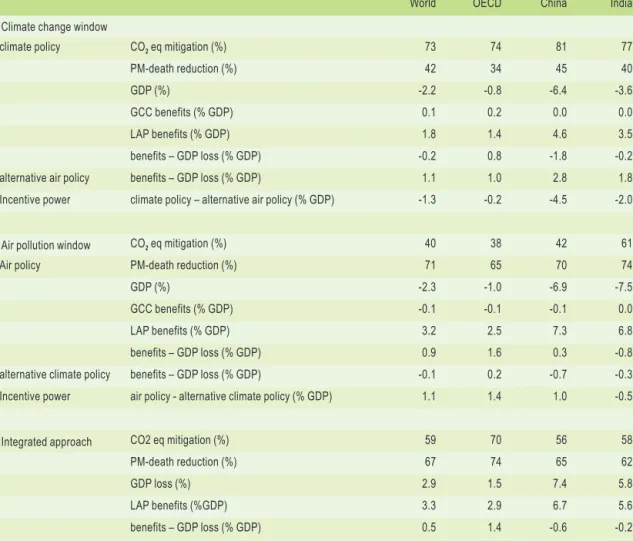
Table 1 summarizes the impacts of different variants of mitigation policies representing the three perspectives in Figure 1. All numbers refer to percentage deviations from the Business-As-Usual (BAU) scenario in the year 2050 for the OECD, China and India and also for the world as a whole. The assumptions of the BAU scenario are described in OECD (2008). Table 1 presents both the number of premature deaths and CO2 eq. emissions and the monetized impacts (GDP losses from

abatement, benefits of prevented damage from global climate change and local air pollution). In the climate change window, the policy package provides a cost-effective way of reducing global CO2 eq. emissions in 2050 to 50% below the 2005 level (equal to a 73% reduction of the

BAU emission level in 2050). In the air pollution window, the policy package aims to reduce the global number of premature deaths caused by chronic exposure to outdoor PM2.5 concentrations

in rural and urban areas by 25% of the 2005 level. 2)_{In the integrated approach the model is used} to determine the policy package that maximizes global welfare, given the cost of mitigation and the disutility associated with global climate change and local air pollution (and hence the benefits of mitigation).

2 This global figure is based on the aggregation of regional figures derived as uniform percentage deviation from a time profile of the integrated approach (see Appendix II).

Policy perspective on climate change and air pollution

Global climate change (GCC)

mitigation policies Local air pollution (LAP)mitigation policies Impact 1

Additional impact 2

Impact 2

Climate change window Air pollution window

Additional impact 1

Integrated approach

Air pollutants (SO₂, NO_X, VOC, NH₃, PM) Greenhouse gas emissions

(CO₂, CH₄, N₂O)

(15)

Summary

Co-benefits are calculated as the monetary value of the disutility it causes (as % GDP), and also as the avoided costs of an alternative policy achieving the same co-benefit at the lowest possible cost. Within the climate change window and the air pollution window, net benefits are calculated for both types of policies. The difference between these two figures, referred to as the ‘incen-tive power’, represents the net benefits of climate or air policies when considering co-benefits as avoided cost instead of monetized disutility. If the incentive power is a positive number, the benefits and co-benefits (avoided costs) together are large enough to compensate the cost of the policy.

In the integrated approach, no distinction is made between primary benefits and co-benefits. All effects are included and weighed against each other in order to determine an optimal policy, maximizing global welfare.

Scope of the study

There have been several assessments focusing on the interactions between policies for global climate change and local air pollution. As the notion of co-benefits originated in climate policy discussions, most of these assessments have focused on the co-benefits in terms of a reduction in local air pollution that stem from GHG mitigation policies (like in the climate change window). A key conclusion is that GHG mitigation could yield large near-term co-benefits in terms of reduced risks to human health (OECD, 2008). Moreover, in developing countries, the number of

Table 1 Main results in 2050 of different windows of policies (% change compared with BAU)

World OECD China India

Climate change window

climate policy CO2 eq mitigation (%) 73 74 81 77

PM-death reduction (%) 42 34 45 40

GDP (%) -2.2 -0.8 -6.4 -3.6

GCC benefits (% GDP) 0.1 0.2 0.0 0.0

LAP benefits (% GDP) 1.8 1.4 4.6 3.5

benefits – GDP loss (% GDP) -0.2 0.8 -1.8 -0.2

alternative air policy benefits – GDP loss (% GDP) 1.1 1.0 2.8 1.8

Incentive power climate policy – alternative air policy (% GDP) -1.3 -0.2 -4.5 -2.0

Air pollution window CO2 eq mitigation (%) 40 38 42 61

Air policy PM-death reduction (%) 71 65 70 74

GDP (%) -2.3 -1.0 -6.9 -7.5

GCC benefits (% GDP) -0.1 -0.1 -0.1 0.0

LAP benefits (% GDP) 3.2 2.5 7.3 6.8

benefits – GDP loss (% GDP) 0.9 1.6 0.3 -0.8

alternative climate policy benefits – GDP loss (% GDP) -0.1 0.2 -0.7 -0.3

Incentive power air policy - alternative climate policy (% GDP) 1.1 1.4 1.0 -0.5

Integrated approach CO2 eq mitigation (%) 59 70 56 58

PM-death reduction (%) 67 74 65 62

GDP loss (%) 2.9 1.5 7.4 5.8

LAP benefits (%GDP) 3.3 2.9 6.7 5.6

(16)

premature deaths will increase over time because of urbanization and the increasing share of the elderly in the population, despite that local air pollutant control measures will come into effect. Furthermore, the ratio between co-benefits related to local air pollution and the marginal costs of GHG mitigation are greater in developing than in developed countries, partly due to higher increase in air pollution in the former group of countries.

There are only a few analyses that investigate the co-benefits of climate policies from the point of view of avoided cost of air pollution policies. Moreover, there are not many studies that look at the interrelations between global climate change and local air pollution through the air pollu-tion window or in an integrated approach. In this report, these issues are explicitly addressed through simulations that were made with an extension to the Model for Evaluating the Regional and Global Effects of GHG Reduction Policies (MERGE) to include outdoor local air pollution. The model takes into account the main pollutants that have an impact on human health, except for the impact of ozone. The extended model was used to simulate the costs and benefits of miti-gating global climate change and local air pollution in a general equilibrium, dynamic, multi-regional and multi-sectoral framework.

The climate window

Co-benefits of climate policies are significant and increase over time

Simulations in the climate window show that GHG mitigation policies result in a reduction in the number of premature deaths due to air pollution compared with the BAU scenario by around 40% globally in 2050 (Table 1). In the OECD this percentage is smaller than in India and China. This is partly because local air pollution in the OECD countries is mainly driven by the demand for transport services, whereas outside the OECD a major driving force is coal burning by house-holds. This analysis includes the impact of emissions from household energy consumption on outdoor pollution, but not from indoor pollution. In the next 20 years, cheap GHG abatement opportunities in developing countries are more in the electricity than in transport sector, at least compared with OECD countries. Thus, the resulting emission reductions have less impact on local air pollution in the former than in the latter.

Furthermore, exposure to local air pollution is usually higher when pollution results from many small sources in transport and domestic sources than from large-scale power plants. However, as illustrated in Table 1, the co-benefits are higher in non-OECD than in OECD countries for more stringent emission reductions or over longer time scale. This is the case when relatively cheap CO2 abatement opportunities in the electricity sector in non-OECD countries are exhausted, and

OECD countries run out of options to reduce local air pollution through GHG mitigation policies. Beyond 2050, however, co-benefits tend to stabilise and even decline slightly in terms of number of deaths as well as in monetary terms. The main reason is that the non-energy related local air pollution substances such as NH3 become a more dominant source of pollution than energy

combustion so that climate policy can no longer significantly reduce emissions responsible for local air pollution. Hence, the co-benefits do not increase further and may even decrease. Co-benefits of climate policies will increase in the longer term only in non-OECD countries Aging and strong urbanisation result in a more vulnerable population in non-OECD regions. Therefore, the co-benefits in terms of prevented deaths increase over time. To compare co-bene-fits with the cost of mitigation policies, the number of prevented premature deaths is multiplied

(17)

Summary

by the value of a statistical life. The value of a statistical life is assumed to be proportional to GDP per capita in a region. High economic growth and a resulting high value of a statistical life will therefore boost the co-benefits in non-OECD countries further. Finally, with the assumed uniform CO2 eq. price, emission reductions would be higher in non-OECD than in OECD

coun-tries. When expressed as percentage of GDP, co-benefits are also larger in non-OECD than in OECD countries.

Up until 2050, the co-benefits of climate policies alone will probably not provide sufficient incentive to participate in climate mitigation strategies.

It appears that co-benefits can cover a significant part of the costs. The extent to which co-bene-fits of climate mitigation policies offer economic incentive for countries to participate in climate policies depends on two factors. First, the extent and the value of the co-benefits is important. In 2050, in the OECD the benefits of air pollution are large enough to totally compensate for the GDP loss of the GHG mitigation policies. In India and China and also for the world as a whole, this is not the case, although the benefits to a large extent compensate for the mitigation cost. Second, it is also important to consider the cost of achieving the same level reduction of local air tion through direct policies. If these costs of direct policies are less than the monetized air pollu-tion benefits, these should be considered as the co-benefits achieved. For all regions this implies that indeed the co-benefits increase the incentive to participate in a climate agreement up to 2050, but they are not enough to fully compensate for the cost of mitigation policies. After 2050, the gains from GHG mitigation are expected to become large and to outpace the mitigation costs. Air pollution window

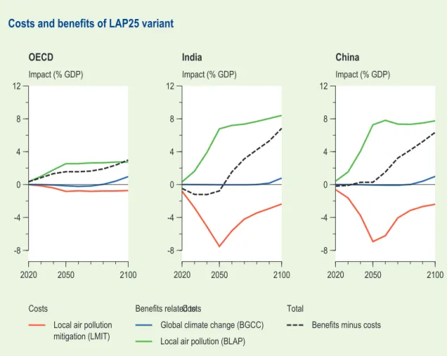
The co-benefits of stringent air pollution policies are significant, and provide an incentive for many regions to pursue this air pollution strategy.

In many regions, there are large incentives for countries to directly control local air pollution (or to go through the air pollution window). Local air pollution could be effectively reduced by add-on cadd-ontrol technologies, which would not reduce GHG emissiadd-ons. Significant reductiadd-ons in the level of local air pollution, as shown in Table 1, however result in substantial reductions in GHG emissions, indicating that structural energy adjustments are pursued.

In all three regions, total benefits of reduced air pollution outweigh total cost in the long run. In the short-term, net benefits are only found in the OECD, whereas in China, local air pollu-tion policies are profitable from 2030 and in India this is not the case until 2050. Because of the relatively high reduction in emissions of air pollutants and a high energy intensity in India, the country is confronted with high GDP losses offsetting air pollution benefits. As a result, the reduction in emissions of CO2 is also relatively high in India.

Although GHG emissions are substantially reduced as a co-benefit of air pollution policies, until 2080 this does not result in a reduction in global average temperature rise. In the long run (2100-2150), global temperature stabilizes at a level well below the long term global temperature level in the baseline. The counterintuitive development in global temperature is the result of the cooling effect of SO2. Due to the reduction target for air pollution, SO2 emissions are reduced

significantly (worldwide over 80%). As a result, the cooling effect of sulphate aerosols, which in total is estimated to reduce global average temperature by about 0.7 degrees, disappears rapidly. In 2050 the global climate change co-benefits are negative.

(18)

Integrated approach

The integrated long-term cost-benefit approach balances the means to lower simultaneously the adverse impacts of climate change and air pollution and shows significant climate benefits only after 2050.

In summary, these simulations and results from the literature review suggest that for coun-tries giving priority to GHG mitigation, the local air pollution co-benefits provide an additional incentive by off-setting a proportion of the GHG mitigation costs. These co-benefits could be larger than currently estimated since most estimates omit the possible co-effects of GHG mitiga-tion on indoor air pollumitiga-tion, which is expected to be large in countries such as India and China (IPCC, 2007). Still, it remains to be seen whether these indoor induced co-benefits are large. As already stated, the GHG mitigation strategy reduces CO2 emissions from households only in the

more stringent cases, and in the longer term. In addition, the carbon price will likely yield only small co-benefits in terms of reduced indoor air-pollution as there may be a switch from coal to biomass. Keep in mind that the burning of biomass also generates emissions of particulate matter.

Moreover, the outdoor air pollution benefits could also be higher, if the baseline PM10 emissions

were higher. If so, the reductions in CO2 eq. emission would go hand in hand with higher

reduc-tions in PM_2.5 emissions. 3) However, the co-benefits could also be lower if the attributive risk parameter - linking average concentrations of PM2.5 to the number of deaths – is lower. 4) The

literature is not conclusive on this issue. With lower attributive risk parameters, the damage of local air pollution in the baseline and the co-benefits of the GHG mitigation strategy will also be lower.

However, for countries that give priority to air pollution control over climate change policy, co-benefits of climate policies are still positive but unlikely to provide sufficient incentive to participate in a climate agreement. Local air pollution control policies give a higher return on investment. This result is independent of any assumption on the value of a statistical life, because the co-benefit of climate policy is offset by the direct benefit of the much cheaper air pollution policy.

Nonetheless, countries that plan to significantly control local air pollution would de facto reduce GHG emissions. Finally, as local air pollution and global climate change are both driven by fossil fuel combustion, there are synergies and higher returns on controlling both GHG and local air pollution (integrated approach). Hence for countries that give priority to mitigate the adverse impacts of local air pollution, there is an incentive to also invest in mitigation policies and to maximise benefits across these areas. The synergies can be seen to especially depend on the

3 In this sense, the co-benefits are relatively low because of the relatively low emissions in the BAU scenario. This is consistent with the recent dynamics in the regulation of LAP substances in China. In 2007, the annual rise in CO2emissions was 8%, whereas SO2emissions fell by 10% (MNP, 2008).

4 More deaths are estimated in this analysis than in the OECD environmental outlook. The main reasons are firstly, the anthropogenic contribution to pollution is higher, and hence the number of premature deaths are based on concentrations larger than 0 μg/m3_{, instead of the} approach based on WHO (2004) for urban areas to measure only the number of deaths above 7 ug/m3. Secondly, the number of diseases assumed to be relevant not only concerns mortality from cardiopulmonary disease and lung cancer, but is includes all mortality impacts from exposure to local air pollutants.

(19)

Summary

level of value of a statistical life, but even the climate sensitivity parameter. If the value of a statistical life is high, then the co-benefits are also high, and vice versa.

Finally, this report demonstrates that the benefits of local air pollution reduction significantly outweigh those of global climate change mitigation in the integrated approach. The benefits of prevented climate damages only show to be significant beyond 2070. Hence, the discounted benefits of local air pollution certainly outweigh those of global climate change. Still, it is not argued to only restrict energy policy making today to what should be the first priority, local air pollution control, and wait with the reduction of greenhouse gas emissions, but instead to design policies that simultaneously address both these issues, as their combination also creates an additional climate change bonus. It seems from the analysis of this report that climate change mitigation proves to be an ancillary benefit of air pollution reduction, rather than the other way around.

(20)

(21)

Introduction 1

1 Introduction

There are strong linkages between global climate change (GCC) and local air pollution (LAP). Emissions from the combustion of fossil fuels contribute significantly to both GCC and LAP. These key environmental issues are discussed extensively in the international political arena: the first notably in the United Nations Framework Convention on Climate Change (UNFCCC) and the second in, for instance, the United Nations Economic Commission for Europe’s task-force on Long-Range Transboundary Air Pollution (UNECE-LRTAP).

Options to mitigate GCC may show strong co-benefits in terms of less LAP and vice versa. For example, policies to limit transport emissions and congestion will both improve air quality and simultaneously have positive consequences on GHG emissions. However, this is not always the case. Greenhouse gas (GHG) emissions can be cut by equipping fossil fuel power plants with CO2 Capture and Storage (CCS) technology only addresses greenhouse gases and usually not

emissions of air pollutants. CCS equipment installed in isolation therefore alleviates GCC but not LAP. End-of-pipe abatement techniques reduce emissions of local air pollutants (SO2, NOx, NH3,

or particulates) Their application thus contributes to diminishing LAP but not to GCC.

Policies neglecting these co-benefits may be sub-optimal. An integrated analysis of GCC and LAP was carried out to determine the extent to which the co-benefits of climate mitigation policies offer economic incentive for countries to participate in a global agreement to mitigate GHG emissions. The analysis also provides insight into the co-benefits of air pollution policies to offer economic incentive to further reduce on the emissions of air pollutants.

The main issue analysed was the extent to which GHG mitigation costs are covered by the co-benefits in terms of less local air pollution. It seems that climate mitigation costs would be partially covered by the co-benefits if the world community could agree a uniform carbon price. Further, GHG mitigation policies will only increase co-benefits outside the OECD region in the longer term or by means of stringent policies. A related question is the impact of policy design (such as CO2 eq. emissions trading) on these co-benefits.

For this analysis of the dual GCC-LAP problem, the global top-down model MERGE was used. MERGE (Model for Evaluating the Regional and Global Effects of greenhouse gas reduction policies) has been developed by Manne and Richels (1995). This climate change model includes sufficient bottom-up technology features. For the purpose of this study, the model was expanded with a module dedicated to local air pollution including mathematical expressions for:

Emissions of local air pollutants (SO

• x, NOx, NH3 and primary PM) in all sectors,

Chronic exposure of the population to increased lAP (concentration of pollutants), •

Premature deaths from chronic

• LAP-exposure in urban and rural areas,

Monetary estimates for damage resulting from premature

• LAP deaths.

The LAP module was calibrated to estimates from studies by the World Health Organization (WHO, 2002; 2004) and the RAINS consortium (Amman et al., 2004), as well as several other sources (Pope et al., 2002; Holland et al., 2004). Since cost estimates of GCC and LAP damage as well as most of our other modelling assumptions are subject to uncertainties, a sensitivity analysis was performed on key modelling assumptions. These include discounting assumptions, the number of premature LAP-related deaths, and monetary valuation of these deaths.

(22)

The welfare benefits from preventing LAP-related damage are important in the modified version of MERGE used in this study. Benefits can be realized by reducing emissions of SO2, NOx, NH3,

or particulates. Emission reductions involve end-of-pipe abatement measures, or a switch from fossil fuels to cleaner forms of energy. When benefits exceed costs, an incentive is created for reducing emissions of local air pollutants. A similar and synchronous balancing between costs and benefits occurs for CO2 emission reductions. At the same time, a balancing occurs between

the incentive to act on LAP respectively GCC, while interactions and spillovers between these two add to the overall optimisation process.

The analysis employed a stylised version of LAP which is restricted to outdoor health impacts of air pollutants and excludes acidification and indoor air pollution. There are also several abstrac-tions in this analysis:

The focus is on emissions from fossil fuel combustion in the electricity and non-electricity •

sectors, and process emissions for all substances as these impact exposure to PM2.5 but are

also the main source of GHG emissions, and thus the principal driver of both GCC and LAP. The focus is on fine PMs with a diameter of less than 2.5 μm (referred to as PM

• _2.5) which are

responsible for deaths from particulates in the ambient air.

The transboundary aspects of secondary aerosol formations are disregarded because inter-•

regional transport of these pollutants would need to be addressed, and thus require a more in-depth version of an air-transport model. This is beyond the scope of this analysis. Whereas theoretically

• PM can travel thousands of kilometres, the major contribution to local PM concentrations is from emissions close to the source. The high concentrations of primary PM in cities and densely populated urban areas mostly result from transport systems and power plants in the vicinity. Thus, the assumption can be made that reductions in regional PM emissions contribute to a decrease in PM concentrations within the region under consideration only, especially in the light of the very large area modelled.. 5)

There are also a set of significant approximations. We modelled

• LAP at a highly aggregated level because this enabled LAP and GCC to be inte-grated into a single modelling framework. The drawback is that modelling of local air pollut-ants is more rudimentary than for instance in RAINS. The detailed bottom-up abatement cost for EU countries has been reduced to only a few sectors and regions. This approach, however, has the advantage that the economic aspects are more realistic than in RAINS, because the simplification enables simulation of time-dependent abatement technology costs.

The impact on mortality is higher with PM

• 2.5 concentration than with PM10 concentration. As

very little PM2.5 data are available and PM10 data are readily available, these data were used as

proxy for PM2.5 data, as in WHO (2006).

There is probably only a linear relationship between

• PM emissions and concentrations at

intermediate emission levels. The PM concentration depends not only on regionally produced air pollution, but also on local factors such as meteorology. However, at low emission levels, the increase in LAP emissions alters the concentration of PM2.5 very little and thus is mainly

determined by regional PM background values. Nevertheless, this analysis was restricted to a linear dose-response relationship.

5 Regions in MERGE are USA, Western Europe, Japan, Canada/Australia/New Zealand, Eastern Europe and the former Soviet Union, China, India, MOPEC, and the rest of the world. The model employs a time horizon of 150 years (up to 2150) with time steps of ten years.

(23)

Introduction 1

The valuation of premature deaths from chronic exposure to

• PM concentrations is a

conten-tious issue because there are basically two approaches: Value of a Statistical Life (VSL) and Value of a Life Year (VOLY) multiplied by the number of Years of Life Lost’ (YOLL). For the CAFE program, the European Commission decided to adopt the precautionary principle, and used the VSL approach [REFERENCE]. It was also argued that VSL is more statistically reli-able than VOLY. This study used the VSL approach but also tested the robustness of the major conclusions on sensitivity/ uncertainty analysis.

Even though a stylised version of LAP, the model is a starting point for exploring and testing the potential significance of synergy between GCC- and LAP-policies. The study provides a cost-ben-efit framework that derives economically optimal pathways for CO2 and emissions of air

pollut-ants, given parameter values and specific modelling assumptions. These pathways are based on a trade-off between costs of mitigation efforts and benefits of preventing mid-term air pollution and long-term climate change damage.

An overview of the adapted version of MERGE is presented in Chapter 2. This chapter focuses on the adaptation of the original MERGE model with respect to air pollution, as far as it may give rise for a sensitivity analysis of the main findings of the report.

Chapter 3 discusses the perspective of the climate window by exploring the co-benefits of climate mitigation policies, and the perspective of the air pollution window is presented in Chapter 4 by analysing the co-benefits of mitigation policies of air pollution. The broader inte-grated perspective of addressing LAP and GCC simultaneously is taken in Chapter 5 which also addresses the spillovers of CO₂ emissions trading on air pollution policies. The robustness of the main findings is tested in Chapter 6 and main conclusions and recommendations are presented in Chapter 7.

(24)

(25)

Model approach 2

2 Model approach

Quantifying the co-benefits and the incentive power of participating in a global GCC mitigation strategy were analysed with model simulations using the extended peer-reviewed MERGE model. MERGE was originally developed and applied to simulate the impacts on the regional economy, to estimate global and regional effects of greenhouse gas (GHG) emissions and the costs of the emission reductions (Manne and Richels, 2004). The MERGE model was modified (Bollen et al,.2007) to simulate the impacts of outdoor local air pollution (LAP) and for this study LAP was refined to describe the emissions and impacts of primary PM emissions and to take accountof the health impacts of secondary aerosol formation by simulating regional patterns of SO2, NOx,

and NH3 emissions. The model can simulate the costs and benefits of GCC and LAP policies in a

dynamic and multi-regional context.

In MERGE, the domestic economy of each region is represented by a Ramsey-Solow model of optimal long-term economic growth, in which inter-temporal choices are made on the basis of a utility discount rate. Response behaviour to price changes is introduced through an overall economy-wide production function. The output of the generic consumption depends, as in other top-down models, on the inputs of capital, labour and energy. CO2 emissions are linked

to energy production in a bottom-up perspective, and separate technologies are defined for each main electric and non-electric energy option. The amount of CO2 emitted in each

simula-tion period is translated into an addisimula-tion to the global CO2 concentration and a matching global

temperature increment.

The analysis has global coverage and nine geopolitical regions are distinguished. In each region, production and consumption opportunities are negatively affected by damage (or disutility) generated by either GCC or LAP. The cases analysed by MERGE and the solutions obtained assume Pareto-efficiency. Abatement can be optimally allocated with respect to the dimensions of time (when), space (where) and pollutants (what). 6)

2.1 Cost-benefit mode

In Chapters 3 and 4 the cost effectiveness mode of the model is applied by having the model calculate the cheapest way to meet some imposed target, such as CO2 eq. emissions (at the

regional or global level) or the regional number of premature deaths. However in chapter 5 the cost-benefit (CB) mode of the model is applied. Here the equations are highlighted that are most relevant for the CB-mode. In each year and region an allocation of resources include those assigned to end-of-pipe abatement costs related to emissions of SO2, NOx, PM10,, and NH3 :

t,r t,r t,r t,r t,r t,r t,r

C

I

J

K

D

X

Y

=

+

(1)

with Y representing output or Gross Domestic Product (GDP) aggregated in a single good or numéraire, C consumption of this good, I the production reserved for new capital investments, J the costs of energy, K the end-of-pipe abatement costs as added with respect to the original

(26)

MERGE formulation, D the output required to compensate for GCC-related damages, and X the net-exports of the numéraire good. The subscripts t and r refer to time and region, respectively. Solving the cost-benefit problem implies a control system that leads to lower temperature increases and avoided premature deaths. Together they minimise the discounted present value of the sum of abatement and damage costs. 7)_{There is disutility associated with the damages from} GCC, and LAP. This is shown by the following relation expressing the objective function (maxi-mand) of the total problem, being the Negishi-weighted discounted sum of utility:

(

)

∑

t t,r t,r t,r t,r r r

C

F

E

u

n

log

(2)

with n representing the Negishi weights, u the utility discount factor, E the disutility factor associated with GCC, and F the disutility factor associated with LAP,. The loss factor E is:

h cat

T

E

₌

(

1 ₋

(

_∆

/

_∆

)

2

)

₍₃₎

in which ΔT is the temperature rise of its 2000 level, and ΔT_cat the catastrophic temperature at which the entire economic production would be wiped out. The t-dependence is thus reflected in the temperature increase reached at a particular point in time, while the r-dependence is covered by the ‘hockey stick’ parameter h, which is assumed to be 1 for high-income regions, and takes values below unity for low-income regions. The GCC part of MERGE is kept unchanged in its original form, but for the part of this theory section below the focus is on the expanded MERGE model to account for (A) the chain of emissions of SO2, NOx, NH3, and PM10 increasing

their contribution to the PM2.5 concentrations, (B) the increase of PM concentrations provoking

premature deaths, and (C) the meaning of these deaths in terms of their monetary valuation.

2.2 Valuing Air pollution: VSL

Starting at the end of the impact pathway chain, the question is how should premature deaths resulting from chronic PM exposure be monetised. Holland et al. (2004) recommend using both VSL and VOLY, respectively, to value the deaths incurred from PM exposure. The differences between these two approaches are smaller than the values shown in Table 2.1 suggest. Much of the difference disappears when the VOLY values are multiplied by the number of life years lost. Typically for Europe, an average of 10 life years lost under current PM exposure levels can be assumed. In this case, the VOLY approach at median estimates results in a valuation of death approximately 50% lower than in the VSL approach. In this study, the median estimate of the VSL approach in 2000 has been assumed as the benchmark case.

As shown in Table 2.1, VSL in Europe for the base year 2000 is about US$. 1.06 million (2000). The following equation holds for the monetised damage (F) from LAP:

´´µ ³ ¥¥¦ ¤ ,weur ,weur t,r t,r t,r t,r t,r _Y _P P Y C N . F 2000 2000 06 1 1 (4) 7 Y is ‘fixed’. It is equal to the sum of a production function of a new vintage and a fixed old vintage. With respect to the new vintage, there is a putty-clay CES formulation of substitution between new capital, labour, electric and non-electric energy in the production of the composite output good . With respect to the old vintage, it is assumed that there is no substitution between inputs. New capital is a distributed lag function of the investments of a certain year and a previous time step. K is equal to the costs of end-of-pipe abatement, and just one of the claimants of production, and therefore if K increases, then C reduces (which itself is part of the maximand).

(27)

in which N is the number of premature death from chronic exposure to PM, and P the exogenous number of people in a given population.

For non-European regions, VSL is determined by multiplying VSL for Western Europe (WEUR) with the ratio of these respective regions GDP per capita. For future years, VSL is assumed to rise with the growth rate of per capita GDP (income elasticity is one).

The European Commission decided to use the VSL approach instead of the VOLY method for the CAFE program. The VOLY approach latter can be argued to be less statistically reliable while the VSL also better reflects the precautionary principle. This study tested the robustness of the major conclusions through an uncertainty analysis by applying the 56000 of a VOLY times the average number of 10 life-years gained. The valuation of the mortality impacts decline by about 50%. Finally, a sensitivity analysis was conducted of the model simulations with an income elastic-ity of 0.5 as opposed to that employed in the benchmark case (see Viscusi and Aldy, 2003). The counter-intuitive result emerging from this alternative assumption is that low-income countries will have a larger VSL in the short to medium term, whereas in the long term the VSL will be lower that the base case for all countries.

2.3 From emissions to concentrations to deaths

The concentration in each region is derived from the substance-specific contribution of emis-sions to the ambient concentration. Both rural and urban concentrations are added to the regional average. Equation (2) summarizes the relationship between the average yearly PM2.5

concentration in μg/m3_{in year t and region r:}

∑

∈

=

S s str t,r

H

G

,, (5)

With s the index of substances SO2, NOx, PM10, and NH3, and H the substance-specific

contribution to the regional yearly PM2.5 concentration, which is based on the weighted mean of

urban and rural concentrations in the following equation (3):

(

) (

)(

)

(

tr srurb srrur

)

r t s rur r t s urb r t s r t rur r t s r t rur r t s urb r t s r t t,r s

u

E

C

u

C

u

C

u

H

, , , , , , , , , , , , , , , , , , , , , , , , , ,

1 α

α

+

∆

=

+

=

−

+

=

(6) Table 2.1 Valuation of PM deaths in million 2000 US$ . Source: Holland et al. (2004)

VSL VOLY

Median 1.061 0.056

(28)

With u the exogenous time series of the proportion of people living in urban areas in year t in region r,

∆

E

_s_,_t_,_r the growth of emissions of substance s at time t compared to the year 2000, and the substance-specific coefficient α in urban or rural areas to translate regional emission increases to the regional yearly average concentration of PM2.5.

Equations (2) and (3) convert regional emissions of the different substances into PM2.5

concen-trations. The model is linear in emission changes and does not take account of transboundary aspects of air pollution. This simplifies the complex interactions between substances in hetero-geneous areas. 8)

The number of deaths N is estimated from emissions of local air pollutants by assuming that the risk of death increases log-linearly with the ambient concentration of PM2.5 Here, the method

follows the approach used by the WHO to estimate total deaths, or years of life lost, from public PM exposure (WHO, 2002; 2004). One risk coefficient was applied, depending on the PM2.5

concentration, which was multiplied by the population of a given region at a given time. The coefficient was derived from a large cohort study of adults in the USA (Pope et al., 2002). By using this coefficient, the analysis basically relies on fine PM of a diameter<2.5 μm, or PM2.5.

Thus the equation added to MERGE is:

(

)

(

)

t,r t,r t,r t,r t,r

_.

.

_-

-

_G

G

P

c

N

1

059

1

059

1 +

=

(7)

in which G is the PM_2.5 concentration in units of 10 μg/m3_{, P the population of the region , and c}

the crude death rate.

Holland et al. (2005) were followed by estimating all deaths above the nil-effect bottom-line of 0 μg/m3_. 9)_{The values adopted for the regional crude death rates are based on Hilderink (2003)} and take account of relatively more deaths in aging societies and should thus be represented by higher values of c. As expressed in equation (1) with increasing levels for c, the phenomenon of ageing increased the number of premature deaths from PM at a fixed concentration level.

The population will increase over the coming 50 years (globally by +50% and in the OECD region by +20%). Also, regions will be confronted with the issues of an ageing population, and hence the crude death rate will increase (globally by +12% and in the OECD by +8% compared to 2000). This implies that at constant emissions, more people will die prematurely from long-term exposure to PM2.5 concentration driven by the population growth and composition. If

8 The model only relates annual regional emission changes to annual average concentrations. If the transboundary aspects are taken into account, impact would be small on the simulation results because discounted errors in the damage valuation of LAP are small (see Appendix 2). There are several reasons for this. Firstly, the discount rate is on average 3% on the mid-term, hence damage valuation errors will have little impact on the choice variables in the optimsation mode of MERGE. Secondly, the regions are quite large and hence impacts in border locations have a limited impact on the regional average concentration estimate. Thirdly, the regional reduction profiles of emissions are significant in all regions, and thus border location impacts will only affect regional averages if emission reductions differ between two neighbouring regions. Fourthly, although secondary aerosol formation is transboundary, this is not so for primary PM emissions which are one of the main sources for the concentration of PM2.5. Primary PM remains in the vicinity of its source.

9 As opposed to WHO (2004), which measured the number of deaths above a threshold concentration level (7.5 μg/m3_{), an upper boundary} was applied by calculating only the contribution to the number of premature deaths from PM2.5 concentrations.

(29)

emissions of LAP substances remain constant, then deaths will rise by 25% in 2050 in the OECD region (globally by +70%).

Moreover, sustained growth of income will result in an increased movement to urban areas. The urbanisation dynamics will also increase the number of people affected by LAP, see equa-tion (3). If emissions are constant from now onwards, then the number of deaths will increase by between 5 and 10% in the OECD, and by 30% outside the OECD. In summary, in the BAU scenario, besides growth in LAP substances, population growth, ageing population, and urbanisa-tion will increase the number of deaths in 2050 by at least 30% within the OECD, and outside the OECD this will be more than double.

2.4 Implementing the BAU

The mains characteristics of the BAU scenario are growth in population and regional econo-mies, evolution of emission levels of all greenhouse gases (GHGs), which is described in OECD (2008a). The regional time profiles of the LAP substances (SO2, NOx and NH3) follow the OECD

Environmental Outlook (OECD, 2008b), and the regional time profile of primary PM is based on emission intensities from Bollen et al. (2007). 10)

10 The results beyond 2050 are based on an extrapolation of trends of exogenous region and time-specific GDP per capita growth rate. For more details on the numbers, see Appendix I, Table I.1 and I.5.

(30)

(31)

Climate change window 3

3 Climate change window

The main question to be analyzed here will be how much of the of the GHG mitigations costs will be covered by the co-benefits.

This chapter focuses on the GCC50 variant. The main assumption is that global CO2 eq.

emis-sions are reduced in 2050 to 50% of the 2005 level. This GCC50 variant has policy relevance, given the discussion by the G8 and the European Climate strategies. Other variants considered in this study are GCC25 and GCC35 (for more information on the CO2 eq. emission profile,

see Appendix II, Table 1). Simulations have been done for the OECD region, India and China. Comparing the OECD region with two newly industrialising countries is of particular interest because of the tremendous differences in local air quality and the dramatic economic growth in these countries.

Firstly, the monetised impacts of climate action are presented in terms of mitigation cost of GHG emissions, benefits of less global warming and the health co-benefits of improving local air quality (Section 3.1). next, we take a step down and focus on the physical impacts of climate policy: the impacts on GHG emissions and the impacts on air pollutants are presented in Section 3.2 and Section 3.3, respectively. Section 3.4 links co-benefits in physical terms (emissions of air pollutants) to health impacts (deaths) and monetary aspects. Finally, co-benefits are presented as opportunity costs.

3.1 Co-benefits of climate policy

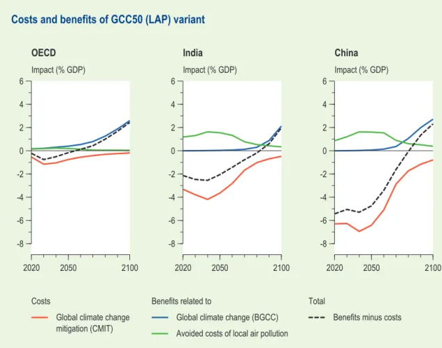
Costs and benefits of climate policy - GCC50 - are presented in Figure 3.1 These include mitigation costs of climate action, the benefits of less global warming and the co-benefits of improved local air quality in the GCC50 variant for the OECD, India and China. Also, the total costs and benefits are given as percentage deviations of GDP from the baseline (BAU).

There is a large time lag between mitigation costs and reaping the benefits from less global warming (“first the pain, then the gain”). Regions suffer an income loss (CMIT) in the first half of the century, and climate benefits (BGCC) only become apparent after 2050.

Co-benefits from better local air quality (BLAP) accrue much earlier but tend to flatten out over time. Air quality improves rapidly with increasing reduction efforts and stabilises in the second half of the century. Mitigation options with a high co-benefit for LAP are relatively cheap and are taken first, for instance, in transport. Only after some time, when greater reductions have to be achieved is attention given to measures with a small impact on air quality such as power generation.

In all three regions, the total of costs and benefits turn positive over time, with mitigation costs declining driven by the reducing cost of the currently expensive technologies of LBDN and LBDE as the global CO2 eq. restriction is greater than 65%. However, this can only be achieved

by 2050 with substantial penetration of the learning technologies. The cost decreases in the electricity sector from EUR 50 to 10 mills per kwH, whereas the more traditional options are relatively more expensive, EUR 40 to 45 mills per kwH.

(32)

There are striking differences between the regions. Mitigation costs (CMIT) and co-benefits (BLAP) are much higher in India and China than in the OECD (See Sections 3.2 and 3.4). Net benefits outweigh the mitigation cost after 2030 in the OECD countries, and after 2050 outside the OECD. CMIT is much higher because of the higher energy intensity in those countries (see Section 3.2). The high co-benefits in India and China are due to the high LAP in the baseline, urbanisation. OECD already has a LAP in place. An aging population (see Appendix I: population dynamics), urbanisation and increasing VSL values make India and China more vulnerable for local air pollution.

3.2 GHG-emission reductions by sector and region

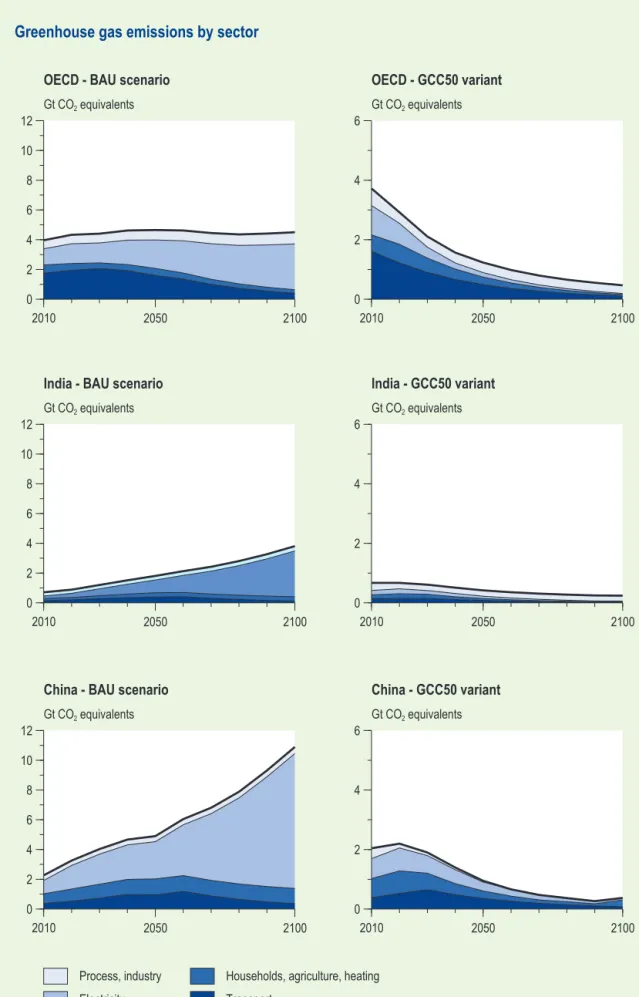
GHG emissions for the OECD region, India and China are presented in Figure 3.2. Four sources are distinguished: power generation (electricity); transport; household demand and heat genera-tion; and processes. Emission profiles are given for the business-as-usual (BAU) scenario and the GCC50 variant.

Currently, emissions from the OECD region are dominant but China will rapidly catch up in the next 20 years, and by the end of this century emissions will be more than three times that in the OECD. India is also growing rapidly but its increasing contribution to global emissions lags behind China and the OECD. Despite the high growth rate, emissions from India are less than China and by 2100 emissions are comparable with the OECD.

2050 2100 -8 -6 -4 -2 0 2 4 6 Impact (% GDP) Costs

Global climate change mitigation (CMIT)

Benefits related to

Global climate change (BGCC) Local air pollution (BLAP)

Total

Benefits minus costs

OECD

Costs and benefits of GCC50 variant

2020 2050 2100 -8 -6 -4 -2 0 2 4 6 Impact (% GDP) India 2020 2050 2100 -8 -6 -4 -2 0 2 4 6 Impact (% GDP) China 2020

(33)

Climate change window 3 2050 2100 0 2 4 6 8 10 12 Gt CO2 equivalents

OECD - BAU scenario

Greenhouse gas emissions by sector

2010 2050 2100 0 2 4 6 Gt CO2 equivalents China - GCC50 variant 2010 2050 2100 0 2 4 6 8 10 12 Gt CO2 equivalents Process, industry Electricity

Households, agriculture, heating Transport

China - BAU scenario

2010 2050 2100 0 2 4 6 Gt CO2 equivalents India - GCC50 variant 2010 2050 2100 0 2 4 6 8 10 12 Gt CO2 equivalents

India - BAU scenario

2010 2050 2100 0 2 4 6 Gt CO2 equivalents OECD - GCC50 variant 2010

(34)

In all regions, emissions from power generation dominate over time. In OECD, emissions from transport are still significant but will dwindle in the course of the century with oil depletion. In the GCC50 variant, GHG emissions reduce considerably. Global emissions in 2030 are 40% below baseline, in 2050 emissions are about 75 % below the BAU scenario and in 2100 there are virtually no GHG emissions (reduction is more than 90% below BAU). Reductions in China and India are higher than in the OECD region. In 2050, the emission reduction by the OECD is 74%, while reduction in India and China is 79% and 80%, respectively. In 2100, the OECD emis-sions in GCC50 are 14% of emisemis-sions in the BAU scenario, while in India, emisemis-sions are 9% of baseline values and in China only 4%. Differences across regions are driven by differences in marginal abatement costs. An efficient global climate regime is assumed. Reductions take place where abatement options are cheapest. Cheap options lie outside the OECD.

With the high energy intensity in India and China compared to the OECD, any reduction percent-age hits harder in these countries; mitigation costs as percentpercent-age of GDP (CMIT) are much higher (see Figure 3.1). In all regions, CMIT increases up to 2050 and thereafter declines because of learning-by-doing. Despite the higher reduction efforts, mitigation costs less because of a forced lock-in of LBDE and LBDN technologies. The reduction percentages are high throughout the century, because the emissions in the BAU scenario increase rapidly, which explains the small differences between regional reductions effort.

2050 2100 0 20 40 60 80 100 % GCC50 variant GCC35 variant GCC25 variant OECD

Reduction of greenhouse gas emissions

2010 2050 2100 0 20 40 60 80 100 % China 2010 2050 2100 0 20 40 60 80 100 % India 2010

(35)

Climate change window 3

In both absolute and relative terms, reductions are highest in power generation (electricity). Emission reduction from household heat generation and from processes and non-CO2 are

rela-tively low. But by the end of the century, emissions have to be reduced to such an extent that emissions from these sources are also considerable.

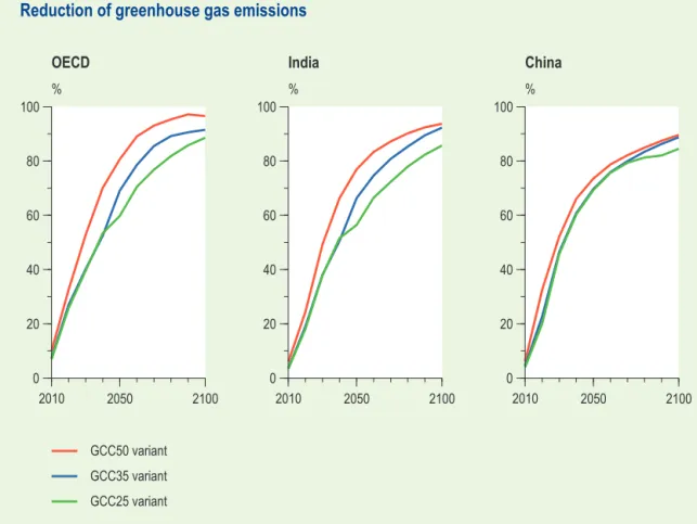
The situation is similar in the other variants GCC35 and GCC50, and reductions relative to the BAU are similar. Emission profiles in BAU, GCC25, GCC35 and GCC50 for the OECD, China, and India are presented in Figure 3.3.

As can be seen, the emission reductions compared to the BAU are large. Reduction by 2050 is 60 to 75%, and increasing to 85 to 98% by the end of this century.

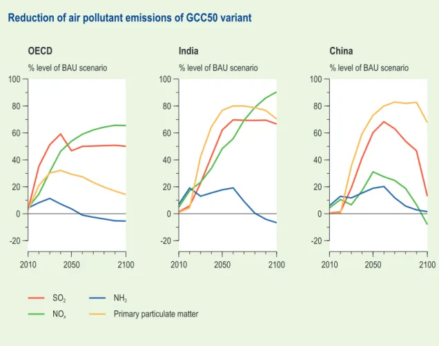
3.3 Emission reductions of LAP

Emissions reductions of SO₂, NO_x, NH₃ and particulate matter in relation to baseline for the three regions - the OECD, India and China – are presented in Figure 3.4. SO2 reductions are

relatively high in the OECD in the first 20 years. OECD relies heavily on measures that affect small point sources such as household heating and energy for transport services, which have a large impact on SO₂ emissions. Oil combustion is the only source of SO₂ emissions (see Table I.6 in Appendix I for emission coefficients of the various technologies).

2050 2100 -20 0 20 40 60 80

100 % level of BAU scenario

SO2 NOx

NH3

Primary particulate matter

OECD

Reduction of air pollutant emissions of GCC50 variant

2010 2050 2100 -20 0 20 40 60 80

China 2010 2050 2100 -20 0 20 40 60 80

India

2010

(36)

Reducing particulate matter (primary PM_2.5) is important in India and China in the latter half of the century when measures in transport are inevitable. PM reductions in the OECD are relatively small given the fact that in the baseline, PM emissions are low due to air quality policies in the past.

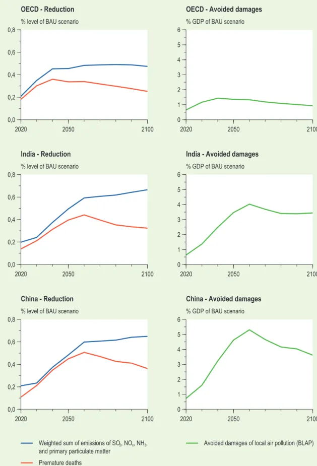
3.4 Reduction of LAP, health and income effects

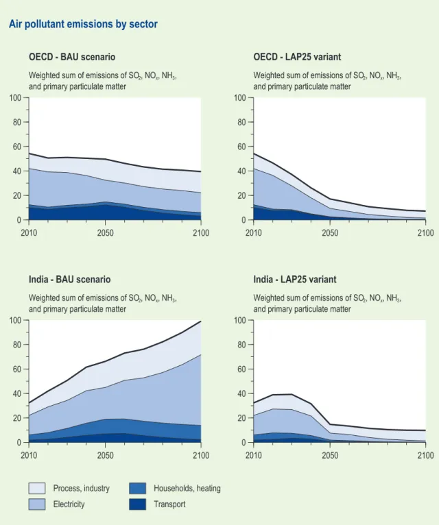
PM reductions (PM sum), reduction in deaths due to local air pollution and the associated income effects of a lower mortality (BLAP) are presented in Figure 3.4. Outcomes of the GCC50 variant are shown for the OECD, India and China. PMsum is a proxy for LAP and is the weighed sum of emissions of SO2, NOx, NH3 and primary Particulate Matter (de Leeuw, 2002).

Health impacts of climate action – fewer deaths due to a better local air quality (LAP deaths) - are closely linked to reductions in PM sum (reducing PM sum also reduces LAP deaths).

Compared to India and China, the population in the OECD is relatively old and more vulnerable. For any given reduction percentage, the impact on LAP deaths is thus higher in the OECD. For example, in 2030 the reduction in PM sum relative to BAU is 24% and the corresponding LAP deaths in 21% lower. In India, in 2030 PM sum is 20% lower but LAP deaths are only 13% lower. As their population ages, India and China become more vulnerable to LAP.

Reduction in PM sum and LAP deaths diverge over time. PM sum is not a perfect proxy of LAP deaths. Reductions in PM sum reflect a regional average. Improvement in urban air quality is better, due to a relative high reduction in PM10. This is not reflected in the regional average. This mismatch becomes more prominent with increasing urbanisation over time. The weighing in PM sum is based on regional average. The divergence is not due to a decline in population, which is assumed to be constant after 2050.

Co-benefits become apparent a little earlier in the OECD region. In these countries, LAP pollut-ants affect CO2 eq. emission reductions especially in the transport sector. In non-OECD countries,

measures in power generation are taken at first with somewhat lower LAP benefits. Only in the longer term in non-OECD countries do the CO2 eq. emission reductions concern the small point

sources such as transport.

Preventing LAP generates in the long run a much higher welfare gain in India and China than in the OECD. In India and China, the benefits in 2050 is 4 to 5% of GDP as a result of less LAP, while in the OECD the accrued benefits are about 1% of GDP. There are two reasons for this. Firstly, a much higher proportion of the population is exposed to LAP. In 2050, mortality due to LAP is higher than 0.2% in India and China, and below 0.1% in the OECD. Secondly, in the long run the percentage reduction in the weighted sum of LAP emissions due to climate action is higher. The increase in income effects in India and China over time is also driven by the assumption that VSL rises proportionally with income (elasticity is one). With the dramatically high growth in India and China, VSL also explodes. By the end of the century, VSL in India and China is even higher than in the OECD. This is based on the assumption that in 2005, VSL in India and China per unit of output was much higher than in the OECD region.

(37)

Climate change window 3 2050 2100 0,0 0,2 0,4 0,6

0,8 % level of BAU scenario

OECD - Reduction

2020

Reduction of emissions, premature deaths, and avoided damages of local air pollution of GCC50 variant 2050 2100 0 1 2 3 4 5 6 % GDP of BAU scenario

OECD - Avoided damages

2020 2050 2100 0,0 0,2 0,4 0,6

Weighted sum of emissions of SO2, NOx, NH3, and primary particulate matter

Premature deaths China - Reduction 2020 2050 2100 0,0 0,2 0,4 0,6

India - Reduction 2020 2050 2100 0 1 2 3 4 5 6 % GDP of BAU scenario

Avoided damages of local air pollution (BLAP)

China - Avoided damages

2020 2050 2100 0 1 2 3 4 5 6 % GDP of BAU scenario

India - Avoided damages

2020