Analysis of clustering approaches to couple hygrothermal material properties with extended degradation risk assessment in masonry constructions

(1)

constructions

degradation risk assessment in masonry

hygrothermal material properties with extended

Analysis of clustering approaches to couple

Academic year 2019-2020

Master of Science in de ingenieurswetenschappen: architectuur

Master's dissertation submitted in order to obtain the academic degree of

Counsellor: Ir. Klaas Calle

Supervisor: Prof. dr. ir.-arch. Nathan Van Den Bossche

Student number: 01407491

(2)

(3)

constructions

degradation risk assessment in masonry

hygrothermal material properties with extended

Analysis of clustering approaches to couple

Master of Science in de ingenieurswetenschappen: architectuur

Master's dissertation submitted in order to obtain the academic degree of

Counsellor: Ir. Klaas Calle

Supervisor: Prof. dr. ir.-arch. Nathan Van Den Bossche

Student number: 01407491

(4)

(5)

Preface

I would like to start by thanking everybody who has contributed to my journey in a certain way.

First, I would like to thank my supervisor N. Van Den Bossche for letting me conduct this research in my own way, given me the opportunity to work on this interesting thesis subject and making my vision clear about what I want to do next. Thanks to K. Calle and I. Vandemeulebroucke for always being prepared to give input and help out with problems along the way.

I would like to thank my friends who always supported me during my journey, always believing, consoling and helping me and especially for creating a fantastic atmosphere in our group.

Last but not least, I would like to thank my parents and family for believing in me and supporting me, even when I was an A level student in making it hard for them.

(6)

(7)

Permission of usage

"The author gives permission to make this master dissertation available for consultation and to copy parts of this master dissertation for personal use.

In the case of any other use, the limitations of the copyright have to be respected, in particular with regard to the obligation to state expressly the source when quoting results from this master dissertation."

(8)

(9)

Analysis of clustering approaches to couple

hygrothermal material properties with extended

degradation risk assessment in masonry

constructions

by

Bruno VANDERSCHELDEN

Masters dissertation submitted to obtain the academic degree of Master of Science in de ingenieurswetenschappen: Architectuur

Promotors: Prof. dr. ir. -arch. N. VAN DEN BOSSCHE Supervisors: Dr. ir. -arch. K. CALLE, ir-arch I. Vandemeulebroucke

Faculty of Engineering and Architecture Ghent University

Department of Architecture and Urban Planning Chairman: Prof. dr. ir- arch. Johan Lagae

Abstract

In order to describe the homogeneity in brickwork, the existing numerical clustering analysis created by Zhao J. is evaluated. The similarity in risk behaviour is questioned since the analysis considers an equally dominant behaviour for each brick property. It makes the objective of this research twofold. Firstly, the homogeneity in brickwork, obtained by clustering analysis, is tested towards similarity in extended degradation assessment for historic masonry walls. Secondly, the question is posed whether there is a similarity in output degradation profiles that can be translated back to a homogeneity in the input parameters, which is generally applicable for the wide variety of brickwork. Therefore, sensitivity analyses on top of an extended examination of several degradation prediction models, are addressed.

Keywords

(10)

(11)

Table of content

ABSTRACT ... 6

1. INTRODUCTION ... 1

2. VARIABILITY IN HISTORIC BRICK MASONRY ... 2

2.1. Brickwork through history ... 2

2.2. Relevant material properties ... 3

2.2.1. Heat storage and transfer ... 3

2.2.2. Moisture storage ... 3

2.2.3. Moisture transfer ... 7

2.3. Translation towards wall assemblies for HAM-simulation ... 9

2.4. Sample construction and definition of input parameters ... 10

2.5. Summary ... 13

3. GENERATING GENERIC BRICKWORK THROUGH CLUSTERING ANALYSIS ... 15

3.1. Clustering analysis ... 15

3.2. Generating generic materials ... 19

3.3. Summary ... 20

4. EXTENDED DEGRADATION ASSESSMENT ... 21

4.1. Mould growth on the inner wall surface ... 21

4.2. Rotting of wooden beams ... 25

4.3. Frost damage in the outer layer ... 28

4.4. Sensitivity analysis ... 30

4.5. Summary ... 32

5. HOMOGENEITY DEFINITION BY CLUSTERING- AND SENSITIVITY ANALYSES... 33

5.1. Homogeneity in brickwork defined by clustering analysis with input parameters ... 34

5.1.1. Conclusion ... 37

5.2. Homogeneity in brickwork based on similarity in degradation profiles ... 38

5.2.1. Similarity of degradation profiles based on statistical values ... 38

5.2.1.1 Median ... 39

(12)

Table of content ii

5.2.1.3 Conclusion ... 45

5.2.2. Translation of similar degradation profiles towards homogeneity in brickwork ... 46

5.2.2.1. Mould degradation profiles ... 50

5.2.2.2. Wood degradation profiles ... 58

5.2.2.3. Frost degradation profiles ... 65

5.3. Summary ... 72 6. CONCLUSION ... 73 References ... 77 APPENDIX A ... 80 APPENDIX B ... 199 APPENDIX C ... 201

(13)

List of Figures and Tables

Figure 1 : Moisture Retention Curve on top with according pore distribution below [1] ... 5

Figure 2: Hygroscopic and overhygroscopic regions in the MRC [1] ... 6

Figure 3: Drying test with critical moisture saturation for brickwork ZB ... 7

Figure 4: Definition of the Liquid Conductivity Curve with different testing methods by Scheffler (2008) [6] ... 8

Figure 5: Abstraction method for historic masonry facades ... 9

Figure 6: Sample of a historic wall assembly... 10

Figure 7: Room temperature and relative humidity generated by Delphin software ... 11

Figure 8 Clustering analysis according to the linkage method [1] ... 17

Figure 9: Normalized dendrogram of Ward method for 17 historical bricks ... 18

Figure 10: Moisture retention curves for generic materials 1 to 4 ... 19

Figure 11: Mould Index classification table [12] ... 22

Figure 12 Wood Decay indicator Merkblad 6-8-15 [15] ... 25

Figure 13: Temperature and Moisture content induced daily dose factors [17] ... 26

Figure 14: Mean decay rating [0-4] at given total dose [17] ... 27

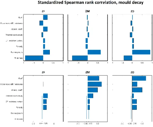
Figure 15: Standardized Spearman rank correlation coefficient, estimates [2] ... 31

Figure 16: Standardized Spearman rank correlation coefficient, p-values. [2]... 31

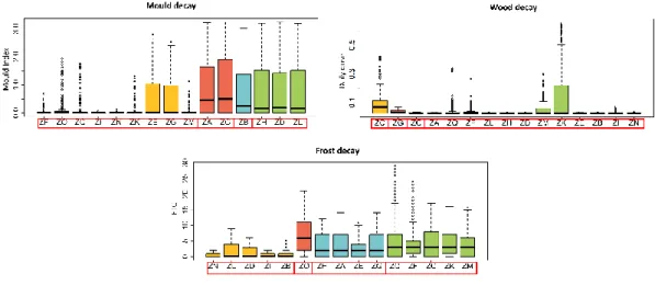
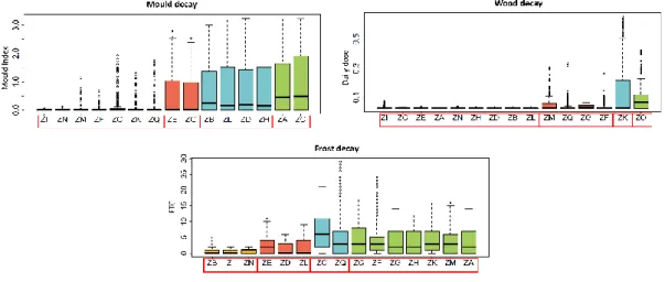
Figure 17: Comparing cluster degradation profiles for Mould decay ... 34

Figure 18: Comparing cluster degradation profiles for Wood decay ... 35

Figure 19: Comparing cluster degradation profiles for Frost decay ... 35

Figure 20: Generic material as prediction method for mould degradation ... 36

Figure 21: Generic material as prediction method for wood degradation ... 36

Figure 22: Generic material as prediction method for frost degradation ... 36

(14)

List of Figures and Tables iv

Figure 24: Clustering scheme for all degradation profiles based on median value ... 39

Figure 25: Ranked degradation profiles based on median clustering ... 40

Figure 26: Ranked degradation profiles per criterion based on median value ... 41

Figure 27: Clustering scheme for all degradation profiles based on average value ... 42

Figure 28: Ranked degradation profiles based on average value ... 43

Figure 29: Ranked degradation profiles per criterion based on average value ... 44

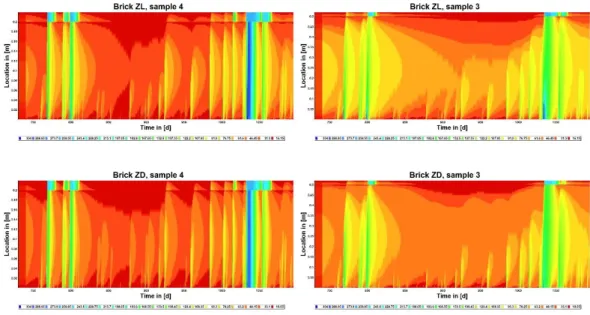
Figure 30: Moisture redistribution for samples 4 and 3 ranked with rising Aw, part 1 ... 46

Figure 34: Mould degradation profiles for sample 5 ... 50

Figure 35: Mould degradation profiles: on the left results for sample 6, on the right results for sample 7 ... 51

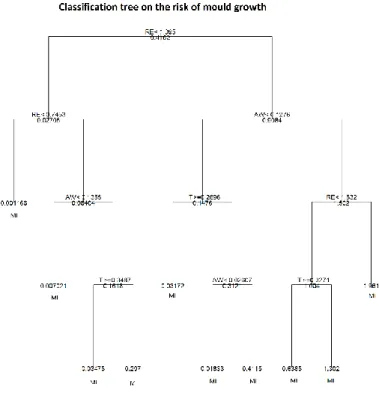
Figure 36: Poisson based classification tree for mould decay based on 3776 simulations ... 52

Figure 37: Standardized Spearman rank correlation for mould decay. Brick: ZF, ZM and ZD ranked with rising Aw ... 53

Figure 38: Overall scatter plot for mould decay ... 54

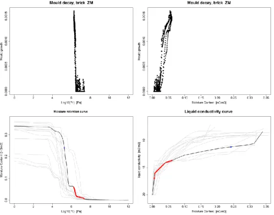
Figure 39: Mould growth at occurring pC and moisture content, on the MRC and LCC for brick ZC ... 56

Figure 40: Mould growth at occurring pC and moisture content, on the MRC and LCC for brick ZC ... 56

Figure 41: Degradation subset based on Aw for mould decay ... 57

Figure 42: Wood degradation profiles for sample 5 ... 58

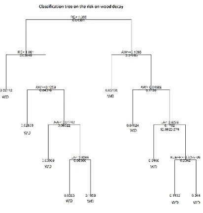
Figure 43: Poisson based classification tree for wood decay based on 3776 simulations ... 59

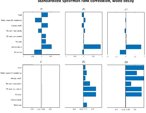
Figure 44: Standardized Spearman rank correlation for wood decay. Brick: ZF, ZG and ZD ranked with rising Aw ... 60

Figure 45: Wood degradation profiles, on the left results for sample 6, on the right results for sample 7 ... 60

Figure 46: Overall scatter plot for wood decay ... 61

Figure 47: Daily doses for wood decay at occurring pC and moisture content, on the MRC and LCC for brick ZL... 63

(15)

List of Figures and Tables v

Figure 48: Daily doses for wood decay at occurring pC and moisture content, on the MRC and

LCC for brick ZK ... 63

Figure 49: Degradation subset based on Aw for wood decay ... 64

Figure 50: Comparison FTC and ICE profiles for sample 7 ... 65

Figure 53: Poisson based classification tree for frost decay based on 3776 simulations ... 66

Figure 54: Overall scatter plot for frost decay ... 67

Figure 55: Standardized Spearman rank correlation for frost decay, Bricks: ZF, ZM and ZD with rising Aw ... 68

Figure 56: Freeze-thaw-cycle at occurring pC and moisture content, on the MRC and LCC for brick ZI ... 69

Figure 57: Freeze-thaw-cycles at occurring pC and moisture content, on the MRC and LCC for brick ZQ ... 69

Figure 58: Homogeneity in MRC for frost decay ... 71

Figure 59: Degradation subset based on Aw coupled with the form of the MRC for frost decay ... 71

Table 1: Property correlation matrix for 22 different bricks [1] ... 12

Table 2: Sample references with according variations and fixed values ... 13

Table 3: Fixed and variable properties of the sample constructions ... 14

Table 4: Mould sensitivity classes [12] ... 23

Table 5: Parameters for different mould sensitivity classes [12] ... 23

Table 6: Decline rate parameters dependant on material [12] ... 24

Table 7: Decay rating according to EN 252 (CEN 2014) ... 27

Table 8: Comparison for calculation methods for the FTC ... 29

Table 9: Sample construction references with according variations ... 49

(16)

Nomenclature

Aw Absorption coefficient Kg/(m2_.sqrt(s)) a Weighing parameter (temperature) m2_/s

C Cluster -

C Moisture Capacity -

CE Specific heat capacity of the dry material J/(Kg.K)

D Daily dose -

D Diffusivity m2_/s

d Distance -

DR Decay rating -

e Fitting parameter (moisture induced) - f Fitting parameter (moisture induced) - g Fitting parameter (moisture induced) -

g Gravitational constant m3_/(s2_.Kg)

h Height m

h Fitting parameter (moisture induced) -

h Heat W/(m2_.s)

i Fitting parameter (moisture induced) -

I Intensity -

j Fitting parameter (moisture induced) -

j Flow/flux Kg/(m2_.s)

k Fitting parameter (temperature induced) - K Permeability or conductivity s l Fitting parameter (temperature induced) -

l Length m

MC Moisture content (daily average) % m Fitting parameter (temperature induced) -

M Mould index -

n Days of exposure d

N Number of modalities -

p Pressure Pa

pC Logaritmic capillary pressure log(Pa) q Fitting parameter (temperature induced) -

q Heat flux W/m2

R Specific gas constant J/(K.mol)

(17)

Nomenclature vii

Greek symbols

α Contact angle ˚ δ Permeability Kg/(Pa.m.s) θ Moisture content m3_/m3 λt Thermal conductivity m/sqrt(s)

μ Vapour diffusion resistance -

ρ Density Kg/m3

σ Surface angle mN/m

τ Toruosity factor -

φ Relative humidity %

Subscripts and superscripts

O Original state a Dry air cap Capillary cond Conductive conv Convective crit Critical diff Diffusive eff Effective g Gas Int Initiation l Liquid mat Material max Maximum MC Moisture content por Open porosity

Q Heat flux

sat Saturation

t time

v Vapour

s Secondes s

S Fitting parameter (steepness of the MRC) -

T Temperature K

t Thickness m

v Wind speed m/s

(18)

Nomenclature viii

Acronyms

CE Specific heat capacity DR Decay rating

ECHE Convective heat transfer coefficient FTC Freeze-thaw-cycles

HAM Heat Air Moisture

IBK (Institut BauKlimatic, Technical University of Dresden

KLEFF Liquid conductivity at effective moisture content

LA Thermal conductivity LCC Liquid conductivity curve MC Moisture content

MEW Water vapour Diffusion resistance coefficient

MIvtt Mould criterion MMD Moisture mass density MRC Moisture retention curve MSD Moisture saturation degree RE Rain exposure

RH Relative humidity

SA Solar absorption coefficient SQ Surface quality

W Wood type

(19)

(20)

1.

1. Introduction

Brickwork is abundantly scattered throughout Europe. The historic masonry façade in Belgium is highly profiled, rendering them an indispensable part of society. Due to harsh weathering conditions and climate change, the protection of these treasures has become a comprehensive and necessary research around the globe. As information about historic brickwork is scarce, the identification of material properties is necessary to supplement the incomplete material data. This can be done by means of material tests such as mercury intrusion, pressure plate test etc., or by performing a numerical simulation that incorporates the possible deviation on the unknown brick property. Both strategies take either a lot of testing- or computational time in order to derive a reliable risk assessment for the wall construction.

To deal with the large variety in brickwork, Zhao J. [1] proposed a clustering analysis which creates homogeneous clusters in brickwork, based on their similarity in input parameters. A generic material could be calculated and would form a representation of all elements in its cluster. The missing properties or the incomplete material data in the renovation application can then be replaced by the most similar generic material or be supplemented with the information of a material that has the closest resemblance. It would help the renovation and retrofit task by reducing the measuring time as well as reducing the computational time during risk assessment.

In the second chapter of this work, a short history explains the emergence of the high variety in brickwork properties, giving the reader an insight on the origin of similarities or dissimilarities. It is important to have a basic knowledge about the parameters that define the exceptional behaviour of porous materials. In the last section, it is explained how the variety of parameters is translated towards a sample construction usable for Heat, Air and Moisture (HAM) simulations. The sample construction was modelled after research done by Calle K. [2].

(21)

Chapter 1: Introduction 2

In chapter 3, the state-of-the-art clustering analysis by Zhao J. [1] is explained. The chapter describes the definition of similarity by means of the Euclidian distance between two individuals. The different methods for cluster analysis are explained and results of the Ward method are compared to the original clustering scheme by Zhao.

In chapter 4, the degradations in historic masonry walls are described. This research considers the occurrence of frost damage, wood rot and mould growth in the historic masonry wall constructions. The state-of-the art prediction models described by Calle K. [2] are evaluated and extended towards a more complete risk assessment.

In chapter 5, the similarities in degradation results and the homogeneity in brickwork are researched. Starting with the numerical clustering analysis of Zhao, which provides a homogeneity in brickwork in terms of input parameters. As the equal impact for each parameter is questioned, the similarities in the degradation profiles are defined in the second section of the chapter, based on the Euclidian distance between several statistical values which represent the degradation distributions. The calculation method provides a similarity definition in the results but lacks the ability to provide the practical field with a clustering scheme, which helps the identification of parameters. Therefore, the last section proposes a methodology, which defines the homogeneity in brickwork by translating the similarity in risk behaviour towards the input parameters by the means of sensitivity analyses.

In the last chapter, a global conclusion is drawn that summarizes the research, focussing on the two objectives of this work. At last, a discussion is opened where the weak points of this research are explained and where the notes for future research are defined.

Appendix A presents a total database of the research, organized per brickwork. General information and brick properties are given, as well as the sensitivity analyses and risk behaviour from the sample constructions.

(22)

2.

2. Variability in historic brick

masonry

2.1. Brickwork through history

Firstly, the history of the brickwork is describes which created the exceptional porous building material. To become the brickwork visible today, it took a long and complicated history. Brickwork was first brought to the Northern and Middle parts of Europe in roman times: the roman soldiers were familiar with the art of brickmaking, while the common man lacked the insights off the production process. After the fall of the Roman Empire, the army vanished and so did the production of brickwork. It is unsure who brought the knowledge of the brick making process back into our region. The church community on the countryside had a great role in the spread of the new brick buildings in their conflict with the guilds in the cities. In the early 15th century, the city landscapes changed as flammable building materials were prohibited and stone buildings became more and more a common sight. With the new brick buildings came new developing methods in the moulding, drying and baking process. The biggest changes took place during the industrial revolution when the production of bricks became a more mechanical process, using horse driven machines and later new fuel supplies. The mining of raw material was depending on the region, as well as the process of baking and the types of ovens used, ranging from a field oven to the Hoffman oven. Brickwork became a material with a great variety of colours and physical properties [3], resulting in a high uncertainty during identification of historical masonry nowadays. As the historic masonry today is exposed to a more harsh climate than ever before, research needs to be done to preserve this history that created the landscape of cities in Belgium and Europe. For a deeper investigation of materials and techniques used in historic masonries, this work refers to Le Noir L. [4].

(23)

Chapter 2: Variability in historic brick masonry 3

2.2. Relevant material properties

The wild history of brickwork ensures that one brick should not be compared with another when the material information is not completely available. As a result, the creation of a uniform guideline for renovation and restauration of historical masonry is still absent in the field. Variables that are influenced by the production of brickwork are heat and moisture specific and both will have a high impact on hygrothermal behaviour. Before a comparative analysis can be defined, a complete understanding of the different brick properties is needed. Therefore, the study provides a summary of the different parameters in the following section.

2.2.1. Heat storage and transfer

The ability of a material to store energy in the form of heat is expressed by the specific heat capacity CE [J/Kg.K], representing the amount of energy [J] that is needed to increase the temperature by one degree Kelvin for one kilogram of material. The transfer of conductive heat through materials is described by Fourier’s law, Eq. (1.):

𝑗_{𝑐𝑜𝑛𝑑}𝑄 = −𝜆(𝜗𝑙) (

𝜕𝑇 𝜕𝑥)

With: 𝑗_{𝑐𝑜𝑛𝑑}𝑄 = heat conductivity flux 𝜕𝑇_𝜕𝑥 = the temperature gradient

The equation incorporates the thermal conductivity LA [W/m.K], indicating the dependency on the moisture content. This can be proven with a simple test where the thermal conductivity of dry air is compared to vapor, the dry air would show a lower value for heat transport. The relation between the moisture content and thermal conductivity during this study was assumed linear.

2.2.2. Moisture storage

Similar to heat, moisture can be stored in the pores of a material. The magnitude of moisture storage, under governing boundary conditions is defined by the moisture storage properties. The outside boundary condition will define a ruling relative humidity (𝜑) or capillary pressure (pc) in the material. Using the moisture retention curve (MRC) representing the relation between the capillary pressure (or relative humidity) and the moisture content, the moisture value in a material can be defined at a certain capillary pressure. Some prefer to use the relative (1.)

(24)

humidity while others will use the capillary pressure. To unify matters, the relation between both is expressed by the Kelvin equation, Eq. (2). The relation in the MRC is mathematically described by various authors, for further reading, see Zhao J. [1]who listed different equations by several authors with their pros and cons.

𝑝𝑐(𝜑) = −𝜌𝑙𝑅𝑣ln (𝜑)

With: 𝜌𝑙 : density of water, 997 Kg/m3

𝑅𝑣∶ gas constant for vapor, 461.5 J/Kg.K

The Kelvin equation shows a logarithmic behaviour for capillary pressure. Therefore, in this work, the MRC is described as the relationship between the moisture content to the logarithm of pc. For further representation, the logarithm of pc will be referred to as pC with a capital C.

The general idea for the MRC derives from the Young-Laplace equation that describes the relation between the capillary pressure and the pore radius:

𝑝𝑐 = −

2𝜎𝑙cos (𝛼)

𝑟 with: 𝜎𝑙 = surface tension of water [N/m]

𝛼 = contact angle of water [ ˚] 𝑟 = Pore size [m]

This equation proves that the pore size distribution, volume of the pore structure for every pore size in the material, is an important variable for the moisture storage ability in porous material. In Figure 1, researched by Zhao J. [1], it is clearly noticeable that the first derivative off the pore distribution defines the trend of the moisture retention curve, as the peaks in the distribution define the location of the steep parts of the MRC.

(2.) 1

(25)

Figure 1 : Moisture Retention Curve on top with according pore distribution below [1]

There are three important levels when referring to the moisture content [m3_/m3_{]: the capillary} moisture content, the effective saturation moisture content and the open porosity, listed in rising moisture level. The capillary moisture content is defined by performing a capillary absorption test. Afterwards, when the porous material is submerged for a longer time to governing boundary condition and atmospheric pressure, the effective saturation moisture content could be reached, which results in an equilibrium of the sample with pure water (relative humidity of 100%). The relation in the MRC reaches its maximum at the effective moisture content. To reach a higher level in the moisture content, the sample needs to be subject to vacuum pressure. By this means, the open porosity could be defined, this moisture content represents all connected pores where moisture can infiltrate.

The moisture retention curve can be seen as a representation of a material that is either in a moisture absorbing or moisture desorption phase. Both will have a different relation, due to the hysteresis effect, which is highly dependent on the material and its pore system. For example, in wood, a high difference in moisture storage during absorption compared to desorption process can be observed, which relates to the pore space geometry and structure. The effect is very complex and forms a major goal in future development to optimise the state-of-the-art Heat, Air and Moisture simulations (HAM).

(26)

Based on the relative humidity in a porous material, the moisture content range as well as the MRC shows two regions: the hygroscopic and the overhygroscopic range. In order to obtain a complete moisture retention curve, insight in the two moisture ranges is required. This can be measured by two laboratory tests. The hygroscopic range consists of the moisture content, varying from zero up to a relative humidity of 95 to 98%. The relation in the MRC for this region is obtained by performing a sorption isotherm test. The overhygroscopic range starts where the hygroscopic range ends and follows up to the effective saturation moisture content. The measuring of the moisture content in this region can be done by a pressure plate test.

Figure 2: Hygroscopic and overhygroscopic regions in the MRC [1]

When performing a numerical simulation, it is preferred to enter a numerical equation for the MRC. Zhao J. [1] has listed several equations ranging from a uni-modal equation, incorporated with the lack of flexibility for multi-pore systems, to the multi-model variant developed by Grunewald. The latter is more flexible when it comes to fitting measured data from a sorption isotherm test and a pressure plate test. The Technical University of Dresden makes use of a multi-modal description, where the weighted sum of the Gauss distribution functions is applied to present an N-modal pore size distribution function.

𝜃𝑙(𝑝𝐶) = ∑ [ ∆𝜃𝑙 2 (1 + erf ( 𝑝𝐶𝑖− 𝑝𝐶 √2𝑆𝑖 ))] 𝑁 𝑖=1

The modality number 𝑁 represents the number of peaks in the pore size distribution. On the same curve, the characteristic logarithmic capillary pressure 𝑝𝐶𝑖 is given by the position of

the pore maxima, while 𝑆𝑖 is the factor affecting the steepness of the curve. [5]

(4.) K θ e f f

(27)

2.2.3. Moisture transfer

Moisture is being transported through the porous material from a dry state until the saturation value is reached. In the lower hygroscopic range, the main transport method is water vapor diffusion. As the relative humidity rises, the moisture content increases as well, hence the occurrence of capillary condensation in the smaller pores. When the overhygroscopic range is reached the water vapor diffusion process is limited in pore space, resulting in the dominance of the liquid phase transport. The latter will continue until the complete pore system is filled with pure water. For an in-depth analysis regarding moisture transport by vapor and liquid, the author refers to Zhao J [1]where the physical processes are thoroughly explained.

The critical value for moisture saturation degree θcrit can be determined by a drying test. Representing the changing point between the first and second trend of the drying curve. The first drying stage is represented with a linear water mass loss over time, caused by convective drying through the porous material. The second drying stage is dominated by diffusion of water vapor and will exponentially lower the drying rate.

Figure 3: Drying test with critical moisture saturation for brickwork ZB

In most cases, the moisture transport in a porous material is described in relation to the absorption ability, represented by the absorption coefficient, Aw [Kg/m2_{.sqrt(s)]. It describes} the amount of moisture stored in the pores in relation to the surface area of the pore system in contact with water and the square root of time.

(28)

Zhao J. [1]has listed the different methods to measure the absorption coefficient from the static laboratory test to a more dynamic field test. He concluded that the results of the on-site measurements have a significant lower accuracy.

The vapor transport in a material consists of two physical phenomena: advective and diffusive water vapor transport. This work focusses on the porous building material “brick” which has a low air permeability, hence the low contribution of the advective water vapor transport. Therefore, this transport mechanism was neglected in the calculations. The main diffusive transport is driven by the diffusion vapor flux, explained by Zhao J. [1]. The vapor transport in a material is compared to the diffusion in still air. As brick contains a pore system that is not perfectly aligned, the diffusion is constricted. The magnitude of the resistance is described by the vapor diffusion resistance factor µ [-]. The resistance factor will account for the geometry and volume of the pore system.

The liquid moisture transport through a porous material can be described by two different properties: the liquid diffusivity [m2_{/s] or the conductivity/permeability [s]. These concepts} have very different meaning as their driving potential have different origins. The diffusivity can be explained by imagining the speed in which an infinitesimal small droplet would spread over the surface of a pore structure, the flow has the moisture content as driving force, while the driving force of the liquid conductivity and permeability is the capillary pressure. The relationship between the conductivity and the diffusivity could be described by the moisture capacity, as the capacity defines the correlation between the moisture content and the capillary pressure. The trend of the liquid conductivity with varying capillary pressure is described by the liquid conductivity curve (LCC). Similar to the moisture retention curve, does the LCC need multiple experiments to define the complete trend.

(29)

2.3. Translation towards wall assemblies for HAM-simulation

Heat, Air and Moisture (HAM) simulations have proven to be a valuable asset to predict degradation in brickwork during renovation and restauration assessment. The difficulty in using numerical simulations lays in the limited detail and variations of wall assemblies one could provide, to keep the computational time acceptable. For the assessment of newly constructed facades, the problem is much smaller since material properties are well known and imperfections, caused by cracks and leakages, are already reduced to a minimal. The challenge is more located in the field of historical masonry facades. Where small adjustments in the translation between reality and simulation can cause great uncertainties on the results of degradation. In order to reduce computational time, the historic wall assembly was abstracted with great care according to Figure 5. The two-dimensional assembly including mortar, cracks, glue etc was represented as one volume of continuous historic brickwork. This assembly helped to build a sample construction to investigate the clustering analysis by Zhao as well as to provide a baseline for the comparative investigation between brickwork.

Figure 5: Abstraction method for historic masonry facades

The simulation software used during this study was Delphin. To start the analysis and simulation, the volume above was subjected to a discretisation process, by dividing the sample into smaller parts with a decreased thickness towards the surfaces of different materials, including air. For each volume, the numerical simulation software established a heat, air and moisture balance by defining the driving force for each time step at each location. The driving force used for moisture storage and transport in Delphin is the capillary pressure. Implying the preference of the liquid conductivity over the liquid diffusivity. Nonetheless, with the aid of the moisture retention curve, the Delphin software is able to calculate the transport properties of the material as well. For a deeper understanding of the physical basis of the software, the author refers to Calle K. [2]and the user manual of Delphin itself [7]. For every simulation performed during this study, was the 3rd_{year evaluated to} reduce the influence of initial conditions in the masonry.

(30)

2.4. Sample construction and definition of input parameters

The comparative study for brickwork needed a sample construction that could represent the different wall properties as well as the different brick properties for a historic masonry façade. Each sample was subject to outside weathering conditions to receive a realistic hygrothermal behaviour. The geometry of the wall assembly was defined first, where the variety of historic masonry assemblies were abstracted to a single leaf masonry with plaster on the inner layer of the brickwork, as presented below. The thickness of the wall was uniformly varied from 150 mm to 500 mm.

Figure 6: Sample of a historic wall assembly

Next in the sampling construction was the group of parameters connected with the exterior climate. The climate itself was fixed at the test reference year (TRY) of Essen located in Germany, provided by the Delphin software database, since this climate is a good representation of the Belgian climate as well. A TRY includes hourly data for: atmospheric counter radiation, direct and diffuse radiation, wind velocity, wind direction, rain flux density on a horizontal surface, exterior temperature and exterior relative humidity.

The work of Calle K. [2]has concluded that the orientation and the rain exposure had the largest impact on different degradations profiles. The two are well connected and only the rain exposure (RE) was assessed in this study, the orientation was fixed on West with 270˚. The rain exposure was uniformly varied from 0 to 2. The range of the RE was chosen large to incorporate bad detailing of gutters as well as overhanging roofs. The coefficient was multiplied by the horizontal rain flux, included in the TRY, to determine the runoff and absorption of moisture by the wall. The long wave emissivity was fixed at 0.9, according to Calle K. [2].

The transfer coefficients at the exterior and interior surface were fixed for every sample. At the exterior, the convective heat and vapour transfer coefficients were respectively 25 W/m2_.K and 2.10-6_{s/m, the indoor were respectively fixed at 8 W/m}2_{.K and 3. 10}-8_{s/m. The magnitude} of the values was considered to have a low impact on the overall hygrothermal behaviour of the wall.

(31)

The boundary condition at the inner wall surface, consists of: relative humidity and temperature. These were calculated with the Delphin generator, based on the governing outside temperature.

Figure 7: Room temperature and relative humidity generated by Delphin software

After defining the wall properties above, the brick properties were defined as follows. The historic building materials for the sample construction were represented by 15 bricks from the IBK (Institut BauKlimatic, Technical University of Dresden) database, referred to as ZA -> ZQ. Z standing for ‘Ziegel’ in German and the second letter was used as an identification method. For individual properties, the datasheet per brick was found in the Delphin database, as well as in Appendix A. In the original work of Zhao, 23 bricks are mentioned but only 17 were fully available in the database. Due to convergence problems in the ice model of Delphin, ZJ and ZP were excluded to prevent misleading results.

Some irregularities regarding the brick properties were found. For example: the constant value for liquid conductivity at effective saturation moisture content (Kθeff) is not represented correctly in the fitting of the liquid conductivity curve. As Delphin will only perform numerical calculation based on the material functions provided, the Kθeff was extracted from the material curve to achieve the same representation during the comparative study.

To achieve a complete comparative study in brickwork, it is important that the discrepancies occurring during property measuring were included in the sampling construction. Therefore, a variance was introduced on the material properties, small enough to prevent interweaving between original bricks. The size of the spread was introduced as the standard deviation, for each property over the 17 historical bricks, divided by 5. Applying this calculation would keep the spread small but still represent a meaningful variance according to testing on the ‘Leopold Kazerne’ in Ghent. The variance was introduced on the material functions (MRC and LCC) by normalizing the original function and applying a scaling factor with value respectively Kθeff and θeff. Hereby, the shape of the curve was respected but the variance was defined by θeff, AW and Kθeff, Eq. (5.).

(32)

The brick properties included in this research were: density, specific heat capacity, effective saturation moisture content, open porosity, thermal conductivity, absorption coefficient, water vapor diffusion resistance and the liquid conductivity at effective saturation point. In the work of Zhao J. [1]and in Table 1, it is clear that several variables have a high correlation. Those relations were incorporated in the Latin Hypercube sampling to build the testing set-up.

Table 1: Property correlation matrix for 22 different bricks [1]

The spread on the open porosity was created by the linearity with θeff. Same for Kθeff which was defined according to the Delphin calculator:

K𝜃𝑒𝑓𝑓=

𝑘𝑘1. 𝐴𝑤2

𝜃𝑒𝑓𝑓

The spread on Kθeff was generated by the variance of Aw and θeff. The 𝑘𝑘1 was the scaling

factor for the liquid conductivity curve and was derived from the original brick properties.

An overview of the used variables and fixed quantities is given in Table 3, at the end of the chapter, for example brickwork ZA. ZA stands for the unit value of the original brick at given property. The different sample construction used during this work is summarized in Table 2, with correct reference name.

(5.) K θ e f f

(33)

Chapter 2: Variability in historic brick masonry 13 Name Thickness Rain exposure coeff. Brick properties [mm[ [-] [-] Sample 1 500 1 Fixed Sample 2 200 1 Fixed Sample 3 500 2 Fixed Sample 4 200 2 Fixed

Sample 5 Variable Variable Variable Sample 6 320 1.5 Variable Sample 7 Variable Variable Fixed

Table 2: Sample references with according variations and fixed values

2.5. Summary

This chapter briefly explained the history of brickwork in Belgium, causing the wide variety in form, colour and definitely physical properties. It became clear that if a brick is compared to another to derive a similar degradation, one should understand the different parameters that define the hygrothermal behaviour of brickwork. After a short introduction to the diverse brick properties, the reader was introduced to the sample construction build to compare different historical brickwork. In next chapter is the clustering analysis explained that forms the state-of-the-art comparative study developed by Zhao J.

(34)

Parameter Units Reference Distribution Range/ Value

Exterior Climate

Orientation [˚] O Fixed 270

Climate [-] C Fixed Essen

Convective heat transfer coefficient [W/m2_.K] _ECHE _Fixed ₂₅ Rain exposure factor [-] RE Uniform 0-2 Moisture transfer coefficient [s/m] Fixed 2.10-6 Ground reflextion coefficient [-] Fixed 0.2 Solar absorption coefficient [-] SA Fixed 0.6 Long wave emmissivity [-] Fixed 0.9 Interior Climate Interior Temperature [˚C] T Fixed Essen

Interior RH [%] RH Fixed Essen

Total heat transfer coefficient inside [W/m2_.K] _Fixed ₈ Exchange coefficient for vapour diffusion at inside [s/m] Fixed 3.10-8 Wall properties Thickness [mm] t Uniform 150-500

Density [Kg/m3_] _ρ _Uniform _{ZA-22.45 , ZA+22.45} Specific heat

capacity

[J/Kg.K] CE Uniform ZA-11.26 , ZA+11.26

θeff [m3_/m3_] _EFF _Normal,

correlated ZA-0.014 , ZA+ 0.014 LN(Aw) [Kg/m2_.sqrt(s)] _AW _Normal, correlated ZA-0.22 , ZA+0.22 Thermal conductivity [W/m.K] λ Normal, correlated ZA-0.036 , ZA+0.036

(35)

3.

3. Generating generic

brickwork through

clustering analysis

In this section, the state-of-the art analysis for clustering, based on material properties is explained and evaluated. In 2012, Zhao J. [1]introduced clustering analysis for different types of materials based on important properties and applications. In the previous chapter, it was explained that a high variety in the properties of brickwork emerged over time. Clustering of brickwork could save valuable time in the measuring process of material properties. These properties are needed to perform a risk assessment during renovation and retrofit applications. In reality, the information for historic building materials is scarce, resulting in the increase of uncertainty, during degradation analysis, and so in a higher computational simulation time.

Clustering analysis creates a generalized material that represents a group of brickwork with similar properties and applications. If a specific material is incomplete in the material property dataset, one could define its cluster and fill out the missing properties with the information of the generalized material or the material closest to it. As the material property would be more specified, the uncertainty in the degradation assessment would be reduced.

3.1. Clustering analysis

To quickly search and investigate materials, it is important to have a good organisation in the material database. Zhao started the organization of the IBK (Institut BauKlimatic, Technical University of Dresden) database by dividing the materials into certain categories.

(36)

Chapter 3: Generating generic brickwork through clustering analysis 16

He classified the materials by their characteristics as well as their usage in building applications. Every material belongs to at least one category with a maximum of three. Examples of categories are: insulation, timber, building bricks, mortars and plasters, natural stones, soil, wood, etc. As this study wants to define a comparative analysis for historical facades, it focusses on the category of building bricks. For each category, the similarities or dissimilarities between individual materials are measured to appoint different clusters, for example “Cluster 2: historical bricks fabricated by the classic loam and clay” in the Building brick category.

The magnitude of similarity in the analysis is measured by the distance between two individuals. Different calculation methods can be used for this purpose, the most common definition is the Euclidian distance. This method measures the distance between the several material properties of two individuals by the Pythagorean formulation:

𝑑𝑖𝑗= √(𝑥𝑖1− 𝑥𝑗1) 2 + (𝑥𝑖2− 𝑥𝑗2) 2 + ⋯ + (𝑥𝑖𝑣− 𝑥𝑗𝑣) 2

The distance 𝑑𝑖𝑗 can be seen as the physical length between two 𝑣-dimensional points in the

Euclidian space. If two materials are in each other’s proximity, they are appointed to the same cluster. The 𝑣-dimensions in the clustering are represented by the following properties:

- Open porosity (θpor)

- Effective saturation moisture content (θeff)

- Capillary moisture content (θcap)

- Moisture content measured at pC 4.78 and 5.60 (θ4.78, θ5.60)

- Moisture content measured at 80% relative humidity (θ80%)

- Water vapor diffusion resistance factor (µ)

- Water absorption coefficient (Aw)

- Thermal conductivity (λ)

- Specific heat capacity (CE)

Not all brick properties are included during the clustering analysis. The exclusion of certain parameters is based on the correlation matrix between variables, see Table 1. The matrix shows a high correlation between the density and the open porosity of bricks. Therefore, the density is excluded as it would only increases the computational time without giving any more valuable insights.

(37)

The magnitude of a variable is reduced by normalization to a unit variance (mean = 0 and standard deviation = 1), decreasing the influence by the weight of the parameter during clustering analysis. Over the normalized database of material properties, the Euclidian distance can be measured by different methods: linkage methods, the Ward method, the K-means method. The first two are described below:

Figure 8 Clustering analysis according to the linkage method [1]

o Single linkage. In this method, the clusters are linked by the nearest neighbour approach, where the distance between two points is minimal. o Complete linkage. Here, the approach is the opposite of the single linkage.

The farthest neighbour is defined by the maximal distance between two points. Consequently, the distances in this method are far greater than in the first method.

o Average linkage. The third method average out the first and the second method, meaning the distance between clustering materials is calculated and averaged. The individuals or clusters with minimal distance will be joined together

o Ward method. The fusion of individuals is performed where the Euclidian distance between centroids is smallest. The centroid of a cluster is the average of the variables of the materials that have already been appointed to this cluster.

During this study, the Ward method was used as it seems to be the most robust manner of clustering with a good handling of outliners in the dataset. The result for clustering analysis, done by R-software, is presented below, where the 17 original bricks are divided into four different clusters. The red boxes represent the different clusters.

(38)

Slight differences can be noticed with the original clustering analysis by Zhao J. [1]. But overall, the same clusters were generated. The irregularities can be caused by the size of the sampling, as Zhao has included more bricks in the analysis. These extra bricks were not fully available in the IBK database and were excluded in this study to prevent misleading results.

Figure 9: Normalized dendrogram of Ward method for 17 historical bricks

The four different clusters represent a wide variety of material properties and are represented as follows:

- Cluster 1 composed out of modern bricks manufactured with new technology

applications.

- Cluster 2 was generated by grouping historical bricks fabricated by the classic

loam and clay.

- Cluster 3 contains the historical bricks that were produced by clay, loam and

additional sand components.

- Cluster 4 is composed by bricks with higher density and lower liquid water

(39)

3.2. Generating generic materials

When different clusters are defined, a generic material representing the cluster elements can be calculated by averaging each material property. In chapter 2, the different properties are evaluated and for the constant variables like density, thermal conductivity etc. the averaging is trivial.

The moisture retention and liquid conductivity curve are more complex, as they were formed by a material generator with varying pC steps according to the pore size distribution of the individual bricks. For a more precise analysis the MRC function was calculated based on Eq. (4.). The necessary parameters were provided by the datasheets from the IBK database. During calculations, the surface tension was assumed to be steady at 0.076 N/m and the contact angle at 0˚. According to Calle K. [2], this method of calculation made averaging for the material functions possible without losing crucial data in the steep section of the MRC.

Figure 10: Moisture retention curves for generic materials 1 to 4

Slight differences between diverse clustering analysis methods can be noticed, but larger differences will occur while analysing different variables, since the clustering analysis is far more dependent on material properties. Consequently, it is valuable to have a fundamental selection in the properties. Adding an extra variable to the analysis will result in the decrease of impact for already presented materials. For example, when adding variables determining the liquid transport through materials, the transport properties will gain impact during analysis while the moisture storage related properties like: effective saturation moisture content, open porosity will lose impact.

0 0.05 0.1 0.15 0.2 0.25 0.3 0.35 0 5 10 Mo is tu re Con ten t [m 3/m 3]

Capillary pressure pC [Pa]

Moisture retention curve cluster 1-4

Cluster 1 Cluster 2 Cluster 3 Cluster 4

(40)

A second problem occurs during averaging of the material functions, in particular with the liquid conductivity curve. In §2.4 is explained how the variance of material functions was implemented in the sample construction. In case the generic material is used, it is important to have a represented method in the scaling of the functions for the whole cluster. During analysis it became clear that slight differences in the degradation profiles appear when changing the calculation method for Kθeff, mainly by the 𝑘𝑘1 factor, determined by Eq. (5.).

The calculation can be done over the whole averaged property of the cluster or it could be calculated for each brick individually and averaged in the last step. Due to a lack of validation for both methods, the second method was used since more similar results to the Delphin calculator were achieved.

3.3. Summary

In this chapter, it was explained how the similarity of historical brickwork can be defined by using the distance between input parameters. After performing the clustering analysis a generic material can be defined that represents the complete cluster. It became clear that the analysis is highly dependent on the used input parameters. Nonetheless, when Zhao performed his clustering analysis, he assumed an equal weight for each parameter. Raising the question whether the equal impact on risk assessment can be assumed. To be able to define the similarity of brickwork in relation to their risk behaviour, the several degradation mechanisms had to be defined. So in the next chapter, several decay mechanisms are proposed with their according prediction models.

(41)

4.

4. Extended degradation

assessment

In this chapter, several degradation risks that arises due to the harsh climate loads on the masonry walls, are assessed. The mould growth, wood decay and frost damage were the focus in this work. Damage caused by pollutant, salt or corrosion was not researched but have a high impact in practical applications as well. Note that none of the criteria have an implementation on strength measurements in the construction, the latter means that the degradation inflected on the structural properties in the masonry wall, was not assessed but should be a goal in future work.

4.1. Mould

growth on the inner wall surface

The first degradation type assessed was the mould growth on the inner surface of a wall, as the quality of the inner surface can be inflicted by excessive humidity and dominant temperatures in wall structures. The degradation does not only jeopardise the quality of the structure and the thermal performances but due to the attendance of pathogens, it also increases the risk for the occupant’s health. Symptoms residents could suffer from are: respiratory complaints, allergenic nausea and much more. This makes it important to control the mould on the inner surface of a construction wall as well as other surfaces in buildings, such as flooring and ceiling.

(42)

Chapter 4: Extended degradation assessment 22

There are several mould predictions models that can be divided into two groups: the static and the dynamic models. The first will only represent the initiation of the biological process while the latter will consider the mould initiation, growth rate as well as the decline in dryer periods. Several models, such as the DIN standards and isopleths were listed and compared by Vereecken E. [12]. The most widely used prediction model, called VTT-model, developed by Hukka and Viitanen [10], forms a dynamic model with two time-dependant variables: the relative humidity and the temperature. Both variables can be calculated by a heat, air and moisture (HAM) simulation and are mostly provided in hourly intervals. The severity of the mould presence is predicted by a mould index running from 0 to 6 with rising degradation. The calculation of the mould index according to the VTT-model is explained below.

Figure 11: Mould Index classification table [12]

First, the critical relative humidity is defined, representing the minimum humidity where initiation of mould growth will start when exposed over a prolonged period of time.

𝑅𝐻𝑐𝑟𝑖𝑡= {−0.00267 𝑇

3_{+ 0.16 𝑇}2_{− 3.13 𝑇 + 100 𝑤ℎ𝑒𝑛 𝑇 < 20℃}

𝑅𝐻𝑐𝑟𝑖𝑡 𝑤ℎ𝑒𝑛 𝑇 > 20℃

The increase or decline in the mould formation is calculated by the use of a differential equation with time steps expressed in hours. In the equation the varying temperature and relative humidity can be included for a more complete assessment.

𝑑𝑀 𝑑𝑡 = 𝑘1𝑘2 168 ( −0.68 ln(𝑇) − 13.9 ln(𝑅𝐻) + 0.14𝑊 − 0.33𝑆𝑄 + 66.02) (7.) (8.)

(43)

The factor 𝑘1 defines the intensity of the growth, W is depending on the timber species (0

for pine and 1 for spruce), SQ implements the surface quality in the assessment (0 for a sawn surface and 1 for kiln dried quality). 𝑘2 defines the moderation of the growth when the mould

index approaches the maximum peak level of mould.

𝑘2= max [1 − exp[2.3(𝑀 − 𝑀𝑚𝑎𝑥)] , 0]

In the latter, the maximum mould index depends on the occurring relative humidity and temperature: 𝑀𝑚𝑎𝑥= 𝐴 + 𝐵. 𝑅𝐻𝑐𝑟𝑖𝑡− 𝑅𝐻 𝑅𝐻𝑐𝑟𝑖𝑡− 100 − 𝐶. (𝑅𝐻𝑐𝑟𝑖𝑡− 𝑅𝐻 𝑅𝐻𝑐𝑟𝑖𝑡− 100 ) 2

The original model of Viitanen was based on pine sapwood, in an improved model [11]the assessment for other materials is added. Hence the following factors in the equations: 𝑘1, 𝑘2,

A, B and C. They are depending on the sensitivity level of the material. Different sensitivity classes are defined in Table 4 and according parameters can be found in Table 5.

Table 4: Mould sensitivity classes [12]

Table 5: Parameters for different mould sensitivity classes [12]

(9.)

(44)

When the mould fungi are not exposed to sufficient moisture or temperature levels, the growth rate will not remain constant but will decrease during these dry periods. A finite delay in mould growth is clearly noticeable after the dry period. The delay is described by the mathematical description dependant on time, starting from the beginning of the dry period (𝑡 − 𝑡1). 𝑑𝑀 𝑑𝑡 = { −0.000133, 𝑤ℎ𝑒𝑛 𝑡 − 𝑡1 < 6ℎ 0, 6ℎ < 𝑤ℎ𝑒𝑛 𝑡 − 𝑡1 < 24ℎ −0.000667 𝑤ℎ𝑒𝑛 𝑡 − 𝑡1 > 24ℎ

Eq. (11.) can take slightly different values for periods longer than 14 days and temperatures below 0 ℃ due to the small number of testing samples in the original test.

Also, the material and its sensitivity level for mould will have a significant influence on the mould decline rate. This influence is implemented using a constant value relative to the material. In the case of historic brick material was an almost no decline, with 𝐶𝑒𝑓𝑓 = 0.1,

assumed during the analysis.

𝑑𝑀 𝑑𝑡𝑚𝑎𝑡

= 𝐶𝑚𝑎𝑡

𝑑𝑀 𝑑𝑡0

Table 6: Decline rate parameters dependant on material [12]

The masonry of historic brickwork in this study was finished with a layer of historic plaster at the inner surface and according to Table 4 the class sensitive (s) was assumed. A note: when the wall is painted it is possible that sensitivity for mould growth is reduced when compared to glued wooden boards or a paper surface, due to mould resistance additives in the paint. After testing the higher sensitivity class (r), the class (s) was still preferred due to better implementation in the comparative investigation.

(11.)

(45)

4.2. Rotting of wooden beams

The next degradation mechanism evaluated was the rotting of wood, as historic buildings are likely to have wooden structures, e.g. the floor construction. These wooden beams are supported by the masonry in the wall construction. As the walls are subject to the harsh outside weathering conditions, the beams are rendered vulnerable for moisture infiltration and under the right temperature conditions can wood decay occur. Different types of fungi can affect the wood. Disfiguring fungi change the colour of the wood but hardly affect the structural properties. More hazardous for construction applications are wood decaying fungi which consume cell wall material of the wood and thus negatively affect the structural properties of the timber. An aspect that is important in this decaying matter is the airtightness around the beam head as shown by research [14]. Therefore, poorly executed air sealing can significantly increase the risk of wood decay due to exfiltration of indoor air containing moist. As a result, the exfiltration at these locations was neglected and assumed to be done properly by the craftsman, during the numerical simulations done in this work. As the beam needs load bearing structure from the masonry, the beam head location was fixed at 120 mm from the inner surface, containing 100 mm masonry as load bearing support and 20 mm plaster. Consequently, when simulations were performed with varying thickness, the distance to the inner surface was constant but the length to the surface adjacent to the outside weather conditions was varied. In the work of Calle K. [2], the wood decay was calculated by assessing the hourly data, surpassing the curve defined in WTA Merkblad 6-8-15 [6-8-15], displayed in Figure 12. A normalized value for wood decay was calculated by the ratio of the total number of data points above the curve and 8760 hours in one year.

(46)

The severity of wood decay, represented by the distance above the curve was not considered. Hence, a deeper assessment of the wood decay was at order. In his dissertation, Vanpachtenbeke M. [16]listed different wood decaying prediction models from laboratory to field testing. Prediction models for wood decay are scarce and can be similarly to mould predictions models be divided in the static laboratory and the dynamic field test. The field testing on Scots Pine sapwood is presented by Brischke and Rapp [17] and later by Brischke and Meyer-Veltrup [19]. In their study the impact of governing moisture content and temperature, on the appearance of wood decay, can be described by a dose-response function. Daily dose D is calculated with a temperature induced component DT, dependent on the average temperature [℃] during the day, and a moisture induced component DMC dependent on the daily average moisture content [%].

𝐷𝑀𝐶(𝑀𝐶) = { 0 𝑖𝑓 𝑀𝐶 < 25% 𝑒. 𝑀𝐶5_{− 𝑓. 𝑀𝐶}4_{+ 𝑔. 𝑀𝐶}3_{− ℎ. 𝑀𝐶}2_{+ 𝑖. 𝑀𝐶 − 𝑗 𝑖𝑓 𝑀𝐶 ≥ 25%} 𝐷𝑇(𝑇) = { 0 𝑖𝑓 𝑇 < 0℃ 𝑜𝑟 𝑇 > 40℃ 𝑘. 𝑇4+ 𝑙. 𝑇3− 𝑚. 𝑇2+ 𝑞 ∗ 𝑇 𝑖𝑓 𝑇 > 0℃ 𝑎𝑛𝑑 𝑇 < 40℃

Figure 13: Temperature and Moisture content induced daily dose factors [17]

The daily dose is then calculated as follows, where the constant a is introduced as a weighing factor for the temperature.

𝐷 =𝑎. 𝐷𝑇(𝑇) + 𝐷𝑀𝐶(𝑀𝐶)

𝑎 + 1 𝑖𝑓 𝐷𝑀𝐶 > 0 𝑎𝑛𝑑 > 0

(13.) (14.)

(47)

The result of the prediction model and the actual results from the field tests where fitted with a Gompertz function and described as a wood degradation rating on Scots pine sapwood. This study used the prediction model for brown rot, as brown rot generally proceeds faster than the white and soft rot in a wood sample.

𝐷𝑅(𝐷(𝑛)) = 4. exp (−exp (1.7716 − (0.0032 ∗ 𝐷(𝑛))

With: n = days of exposure

Figure 14: Mean decay rating [0-4] at given total dose [17]

In the figure above the mean decay rating prediction for the brown rot is presented by the curve. In the numerical testing simulation, the degradation is evaluated for one year. This means at the highest dose of 365, the maximum mean decay rating would be 1.4. The classification of the wood degradation rating is given by following table:

Rating Classification 0 No attack 1 Slight attack 2 Moderate attack 3 Severe attack 4 Failure

Table 7: Decay rating according to EN 252 (CEN 2014)

(48)

In this prediction model, the severity depending on the moisture content and temperature is considered and was preferred over the first method. There, only full damage or total lack of degradation was assumed, with a linear relation between the relative humidity and the temperature. The model by Brischke is the only state-of-the-art prediction model that evaluates the onset of decay that is inherent to experiments on which the prediction is based. Still, there is much to improve as this model is tested in open air with samples subject to shading or no shading. In both scenarios the samples have air flow surrounding them which is excluded in the masonry wall construction. Unfortunately, there is no state-of-the-art prediction model that covers all wood species with varying boundary conditions.

4.3. Frost damage in the outer layer

In the last criterion, the risk involving frost damage induced by freezing water was assessed at a depth of 5mm from the outside boundary conditions. Three possibilities arose: the number of critical freeze-thaw-cycles, the ice mass density or the hygric and thermal stress in the material. The degradation risk induced by frost is highly debated on among researchers.

One strategy is defining the critical degree of saturation introduced by Fagerlund et al in 1975 [21]. As ice expands, the degree of saturation can surpass the point where forming ice creates a pressure on the surface of the pore system, inducing degradation. Simplified, the 91% is considered as critical degree, as ice expands ± 9%. According to Mensinga et al. [22], the critical degree in reality is dependent on the pore structure and in that consideration more material bound.

The increase for frost damage is composed of two general physical driving forces: the ice lens mechanism and the hydrostatic pressure. This work will not give an in-depth analysis of these physical processes and refers to [2]for a more detailed analysis. There are multiple efforts made in the research for analysis of the actual damage of freezing water but these are still in a very preliminary stage and not yet useful in this work. To include the shortcomings of the different driving forces, the criterion considered the freeze-thaw-cycles.

In this work, different ways of calculating the cycles were tested using Delphin. To get a representative result, the simulation needed to be ran with the ice-model enabled. The latter rendered some bricks and wall assemblies vulnerable for convergence problems. The bricks ZJ and ZP, for most wall assemblies, were left out the analysis to prevent faulty conclusion in a sensitivity analysis. The built-in freeze-thaw-cycles calculation in Delphin is based on temperature or ice mass volume. With a temperature-based calculation, a freeze cycle starts when the temperature drops below the dewpoint.