Functional diversity in natural forests along an elevational transect in northern Ecuador

(1)

ALONG AN ELEVATIONAL TRANSECT

IN NORTHERN ECUADOR

Tine Bommarez

Student number: 01500175

Promotor: Prof. dr. ir. Hans Verbeeck

Copromotor: Dr. ir. Marijn Bauters

Tutor: ir. Miro Demol

Master’s Dissertation submitted in the fulfillment of the requirements of the degree of Master in Bioscience Engineering: Forest and Nature Management

(2)

Universiteitsbibliotheek Gent, 2020.

This page is not available because it contains personal information.

Ghent University, Library, 2020.

(3)

ACKNOWLEDGEMENTS

Dear reader,

I proudly present this dissertation as the result of a year of hard labour. The work that lies in front of you would not have existed were it not for the support of some people I would like to thank here.

First of all I want to thank my promotors prof. dr. ir. Hans Verbeeck and dr. ir. Marijn Bauters for giving me the opportunity to participate in this fascinating research project. Together with my tutor ir. Miro Demol they provided indispensable advice and feedback throughout the year, for which I’m very grateful. Furthermore I want to thank Debbie Eraly from BOS+ for her warm welcome in Quito and prof. Selene Baez for her support during the planning of the field campaign and the rest of our time in Ecuador.

This is also the right place to thank my thesis buddy Sebastiaan Van den Meerssche. His marvelous cooking skills, and his slightly mangled attempts to describe the created dishes in Spanglish, provided me and the whole field team with high quality entertainment during our stay. Even when we were already in the process of writing our dissertations, he always remained his jolly self and kept our spirits high, which I really appreciated.

Moreover I would like to thank Germán Toasa, a passionate botanist whose knowledge of the Ecuadorian flora is truly exceptional, and his assistent Stephanie. Germán, gracias por ser nuestro guía y apoyar nuestro trabajo de campo. Sin usted, este estudio no sería lo que es hoy. Stephanie, I will always remember how you galloped effortlessly through the Ecuadorian mountains carrying the bloody tree pruner.

A big thanks to Eva and Emma for their help in the field and back in Belgium. I’d also like to thank everyone from the Mindo Cloud Forest Foundation who helped us both in the field and with logistics: María José, Germanía, Roberto, Fausto and Niko. Qué os vaya bien! I also want to name the people who kept cheering for me every time I bothered them with yet another thesistalk. Lee and Alexander, thank you for your patience throughout these monologues. Your listening ears led me to many insights which eventually found their way into this dissertation.

My parents and Titus get a deserved special mention for always believing in me. Tine Bommarez,

(4)

PREAMBLE COVID-19

A field campaign was conducted during the summer of 2019 in Ecuador to remeasure tree diameters in permanent sample plots and collect leaf, wood and soil samples. The plan was to analyse the chemical composition of these samples during the second semester of the academic year 2019-2020. Due to the emerging threat of COVID-19, Ghent University closed all its laboratories for non-essential research. This halted further sample analyses in the lab. Hence, the planned analyses were only partially carried out. The chemical compo-sition of soil samples was not analysed, whereas leaf samples were only partly analysed. This dissertation was finished on the basis of results that were already available.

This preamble was drawn up in mutual consent between the student and the supervisors and was approved by all of them.

(5)

ABBREVIATIONS

´

a.s.l. Above sea level

AGB Above-ground biomass

BA Basal area

C:N Carbon to nitrogen ratio

CWM Community-weighted mean

DBH Diameter at breast height

FAO Food and Agricultural Organisation of the United Nations

FD Functional diversity

FDis Functional dispersion

FDiv Functional divergence

FEve Functional evenness

FRic Functional richness

HRF Hierarchical-response framework

iWUE Intrinsic water-use efficiency

LA Leaf area

LCC Mass-based leaf carbon content

LES Leaf economics spectrum

LME Linear mixed effects

LNC Mass-based leaf nitrogen content

MAP Mean annual precipitation

MAT Mean annual temperature

MCF Mindo Cloud forest Foundation

MST Minimum spanning tree

POM Point of measurement

PSP Permanent sample plot

SES Structural economics spectrum

SLA Specific leaf area

TMCF Tropical montane cloud forest

TMF Tropical montane forest

WD Wood density

WES Wood economics spectrum

WUE Water-use efficiency

δ13_C _{Stable isotope composition of carbon}

(8)

SUMMARY

Research questions The aim of this study was to investigate both forest taxonomic and

functional diversity patterns along an elevational transect in northwestern Ecuador. Five research questions were addressed. (1) Does an increase in altitude change the floristic properties of tropical montane forest? (2) Does elevation influence functional diversity of tropical montane forests? (3) How does elevation influence the functional trait patterns observed along the transect? (4) For a given altitude, do functional trait values of newly sprouted trees or dead trees diverge from those of the rest of the trees? (5) Which functional traits are predictive for individual tree growth?

Location _{This study was conducted along an elevational transect on the western flank of}

the Ecuadorian Andes. The transect consists of 19 permanent sample plots (PSPs) dispersed among five altitudinal clusters, ranging from 400 to 3200 m a.s.l. The PSPs are located in the provinces of Pichincha and Imbabura.

Methods _{All trees with a diameter at breast height exceeding 10 cm were inventoried.}

Leaf and wood samples were collected for the 80% most dominant species and analysed. For each altitudinal cluster, the community-weighted means of functional traits, the taxo-nomic and functional diversity metrics were calculated and the results were inspected for elevational patterns. Finally, possible correlations between functional traits and individual tree growth were investigated with linear mixed effects models.

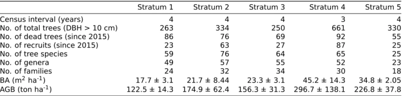
Results We identified 1838 stems from 211 unique tree species, belonging to 147 genera

and 63 families. Tree species turnover with altitude was high. Altitude therefore had a clear effect on taxonomic diversity. Functional traits also appeared to be strongly correlated with elevation. Functional diversity was, unlike taxonomic diversity and functional traits, weakly related to altitude. A higher abundance of tree species with a conservative strategy was encountered at high altitude. The functional trait values of dead trees and recruits did not diverge from the trait values of the rest of the trees. Finally, wood density was predictive for individual tree growth.

Conclusion The tree species in the tropical montane forest of northwestern Ecuador are

highly specialized and have adapted to the environment in which they occur. This is evi-denced by the taxonomic diversity and the differences in functional characteristics of tree species along the transect. We draw attention to the threat that climate change poses to these specialised species.

(9)

SAMENVATTING

Onderzoeksvragen Het doel van deze studie was om de taxonomische en functionele

di-versiteit te bestuderen van natuurlijke bossen gelegen langs een hoogtetransect in Ecuador. Er werd geprobeerd om de volgende onderzoeksvragen te beantwoorden. (1) Heeft hoogte-ligging een invloed op de floristische eigenschappen van tropisch bergregenwoud?

(2) Heeft hoogteligging een invloed op de functionele diversiteit in tropisch bergregen-woud? (3) Hoe beïnvloedt hoogteligging de functionele eigenschappen van bomen langs het transect? (4) Verschillen de functionele eigenschappen van dode bomen of recruten op een gegeven hoogte ten opzichte van de meerderheid van de bomen op diezelfde hoogte? (5) Welke functionele eigenschappen zijn gecorreleerd met individuele boomgroei?

Locatie De studie werd uitgevoerd langs een hoogtetransect op de westflank van de

Ecuadoraanse Andes. Het transect is opgebouwd uit 19 permanente proefvlakken, verdeeld over vijf strata die in hoogte variëren van 400 tot 3200 meter boven zeeniveau. De proef-vlakken bevinden zich in de provincies Pichincha en Imbabura.

Werkwijze In elk proefvlak werden bomen met een diameter op borsthoogte groter dan

10 cm opgemeten en gedetermineerd. Bovendien werden zowel blad- als houtstalen verza-meld van de 80% meest dominante soorten. Na de veldcampagne werden deze stalen geanaliseerd. Op basis van de resultaten werden voor elk stratum taxonomische en tionele diversiteitsmaten berekend. Daarnaast werden de gemiddelde waarden van func-tionele eigenschappen berekend per proefvlak, gewogen voor het grondvlak van elke boom-soort. Er werd nagegaan of deze resultaten gelinkt zijn aan hoogteligging. Ten slotte werden de verbanden tussen functionele eigenschappen en boomgroei onderzocht met behulp van Mixed Effects modellen.

Resultaten Er werden 1838 individuen gemeten en gedetermineerd. In totaal ging het

om 211 unieke boomsoorten, die op hun beurt behoorden tot 147 genera en 63 families. Geen enkele boomsoort kwam op elke hoogte voor en slechts 30% van de boomsoorten kwam op meer dan één hoogte voor. Hoogteligging had dus een duidelijk effect op tax-onomische diversiteit. Ook functionele eigenschappen bleken sterk gecorreleerd te zijn met hoogte. Functionele diversiteit wordt daarentegen in mindere mate beïnvloed door de hoogteligging. De functionele eigenschappen van dode bomen en nieuwe recruten ver-schilden niet merkwaardig van deze van de rest van de staande bomen. Tot slot werd

(10)

zich in sterke mate gespecialiseerd en zijn aangepast aan de omgeving waarin ze voorkomen. Dat blijkt uit de taxonomische diversiteit en de verschillen in functionele eigenschappen van boomsoorten langs het transect. We wijzen op de dreiging die klimaatverandering voor deze gespecialiseerde soorten vormt.

(11)

RESUMEN

Enfoque de la Investigación El objetivo de este estudio fue conocer la diversidad

tax-onómica y funcional de los bosques naturales situados a lo largo de un transecto altitudinal en el noroeste del Ecuador. Se intentó responder a las siguientes preguntas de investi-gación. (1) ¿Afectan las variaciones altitudinales a las propiedades florísticas de los bosques nativos? 2) ¿Afecta la altitud a la diversidad funcional de los bosques nativos? 3) ¿Cómo afecta la altitud a las características funcionales de los árboles a lo largo del transecto? 4) ¿A una altura determinada, difieren las características funcionales de los árboles muertos o reclutas al compararlos con el resto de los árboles? 5) ¿Qué características funcionales están correlacionadas con el crecimiento individual de los árboles?

Localización El estudio se llevó a cabo a lo largo de un transecto altitudinal en el flanco

occidental de los Andes. El transecto se compone de 19 parcelas permanentes divididas en cinco estratos que van desde los 400 a los 3200 metros de altura. Los lugares de muestreo se encuentran en las provincias de Pichincha e Imbabura.

Metodología En cada parcela se midieron y identificaron los árboles con un diámetro a

la altura del pecho superior a 10 cm. Además, se recogieron muestras de hojas y madera del 80% de las especies más dominantes. Después, estas muestras fueron analizadas en el laboratorio. Para cada grupo altitudinal se calculó la media ponderada de los rasgos func-tionales a nivel de comunidad, así como la diversidad taxonómica y funcional. Se comprobó si estos promedios están vinculados a la altitud. Por último, se investigó la relación entre las características funcionales y el crecimiento de los árboles mediante modelos de efectos mixtos.

Resultados _{Se identificaron 1838 árboles. En total se identificaron 211 especies de}

ár-boles, que a su vez pertenecen a 147 géneros y 63 familias, encontrando ninguna especies en cada estrato. El recambio de especies entre estratos es realmente alto, ya que solo el 30% de las especies de árboles se encontraron en más de un estrato. Por lo tanto, la altitud tuvo un claro efecto en la diversidad taxonómica. Las características funcionales también parecen estar fuertemente correlacionadas con la altitud. La diversidad funcional, por otra parte, está influida en menor medida por la altitud. Las características funcionales de los árboles muertos y los nuevos reclutas no diferían notablemente de las del resto de los ár-boles en pie. Finalmente, se encontró que la densidad de la madera es un buen predictor

(12)

altamente especializadas y adaptadas al medioambiente en el que se encuentran. Esto se pone de manifiesto en la diversidad taxonómica y las diferencias en las características funcionales de las especies a lo largo del transecto. Hacemos un llamado de atención acerca de la amenaza que el cambio climático supone para estas especies especializadas.

(13)

INTRODUCTION

Forests cover approximately 30% of the Earth’s surface (FAO and UNEP, 2020). They de-liver ecosystem services indispensable for human well-being such as provision of fresh water, food and timber production and climate regulation (Millennium Ecosystem Assess-ment, 2005). Moreover, tropical forests are highly important for the conservation of global biodiversity (Dirzo, 2001). The study area of this research is located on the western flank of the Andes in northwestern Ecuador. This country is in the top ten countries with most tree species in the world (Beech et al., 2017). The western Andean forests are of utmost impor-tance for biodiversity conservation, as they harbour many species with narrow geographic distributions.

Unfortunately, forests worldwide are subjected to pressures originating from global change and antropogenic disturbances. In 2010, the provinces of Pichincha and Imbabura had a

combined area of 902 000 km2 of natural forests, which is roughly 65 % of their land area.

By 2018, they lost 1414 ha of natural forest, which is the equivalent of 509 000 tons of

emitted CO2 (Global Forest Watch, 2020a,b). Further tree cover loss in this region would

result in additional loss of stocked carbon and disproportionate loss of forest-dependent species (Hill et al., 2019).

Mapping species distributions and estimating carbon storage in these forests can raise awareness on the importance of conserving these forests and halt further degradation and deforestation. For this purpose, an altitudinal transect of permanent sample plots ranging from 400 tot 3200 meters above sea level was set up in 2011 in northern Ecuador, allow-ing scientific research in the framework of a reforestation project conducted by BOS+ and Mindo Cloud Forest Foundation and financed by the Belgian company Telenet. The plots are located in tropical montane forest (TMF), in both reforested as well as undisturbed ar-eas. This experimental set-up allows the study of both reforested sites and the natural climax situation. The project is being scientifically monitored by a cooperation between Es-cuela Politécnica Nacional, Quito, and Ghent University. Previous studies along this transect have rendered interesting insights in terms of tree and liana carbon storage and diversity (Bauters, M., 2013; Strubbe, M., 2013; Demol, M., 2016; Bruneel, S., 2016; Meeussen, C., 2017; Thierens, E., 2017; Pauwels, J., 2018).

The objectives of this field campaign were multiple. First, the demographic rates in TMF was investigated. Comparing the data from the first inventory in 2015 with the new data for plots at a particular altitude allowed us to study vegetation dynamics (growth,

(14)

recruit-evolutions in the size of the carbon stock. This research topic was further elaborated upon in the parallel thesis by Sebastiaan Van den Meerssche.

We formulate five research questions to target in this thesis:

1. Does an increase in altitude change the floristic properties of tropical montane forest? 2. Does elevation influence the functional diversity of tropical montane forests?

3. How does elevation influence the functional trait patterns observed along the transect? 4. For a given altitude, do functional trait values of newly sprouted trees or dead trees

diverge from the properties of the rest of the standing trees? 5. Which functional traits are predictive for individual tree growth?

For the purpose of answering the aforementioned research questions, leaf and wood sam-ples were collected in the forest reserves along the elevational transect. In addition, we enhanced the precision of tree species determination with the aid of a local botanist. This work consists of seven chapters. Chapter 2 provides a concise overview of the existing literature related to the topic. In Chapter 3, a detailed explanation of the procedures used during the field work and lab analysis can be found. Chapter 4 summarizes the obtained results, which are being discussed further in Chapter 5. In Chapter 6, the main conclusions of this research are given. We end with Chapter 7, containing some brief suggestions for further research along the transect.

(15)

LITERATURE REVIEW

Tropical forests occur roughly between the tropics of Cancer and Capricorn and are char-acterised by year-round high temperatures (Dirzo, 2001). As moist tropics harbour an es-timated 50% of the global species richness, these ecosystems are extremely important for the conservation of biodiversity (Dirzo and Raven, 2003). The tropical forest is an umbrella concept harbouring many types of forests. There is no such thing as "the tropical forest". Different types of tropical forests were categorised according to gradients in for example moisture or seasonality (Montagnini and Jordan, 2005).

2.1 Tropical montane forests

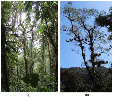
A classification suggested by Foster (2001) relies on changes in elevation. While ascend-ing a tropical mountain, forest ecosystems shift from lowland rainforest to lower montane rainforest and subsequent to upper montane rainforest. In presence of frequent cloudcover a peculiar subtype of tropical montane forest can occur, named tropical montane cloud forest (TMCF). Many definitions for TMCF circulate highlighting different features of this for-est type. Hamilton et al. (1995) emphasise the difference in stand structure compared to tropical lowland rainforest: trees are smaller and more stunted, stem density is higher and epiphytes become more abundant with altitude, as opposed to lianas (Figure 2.1).

In large inland mountain ranges like the Andes, TMCF is typically found between 2000 and 3500 meters above sea level (m a.s.l.), but it can be found as low as 500-1000 m on isolated peaks or closer to sea (Hamilton et al., 1995). This phenomenon is known as the

mass elevation effect_{: on smaller mountains the cloud-base is formed at a lower altitude}

than on large mountain masses because of the lower uptake of solar radiation and higher humidity levels on small mountains in coastal areas (Bruijnzeel et al., 1993; Flenley, 1995).

In 2000, about 1.4% of the world’s tropical forests (≈ 215 000 km2) was estimated to be

TMCF with roughly 40% located in the Americas (Bruijnzeel et al., 2011b). Maps of global TMCF distribution are produced by combining global forest cover assessments with global elevation data and regionally specific altitudinal limits of cloud forests (Bubb et al., 2004; Bruijnzeel et al., 2011a). The most recent maps estimate the TMCF distribution using data obtained through remote sensing (Figure 2.2) (Wilson and Jetz, 2016).

(16)

Figure 2.1: Tropical montane cloud forest in the ecologicale reserve El Cedral (Ecuador). The stand

structure is characterised by (a) persistent cloud cover, small and stunted trees and (b) numerous epiphytes. Photographs taken by author in August 2019.

Figure 2.2: Distribution of tropical montane cloud forest in South and Central America. The color of

a region reflects the local probability of the occurence of tropical montane cloud forest in a quadrat

of 1 km2. The relative occurence rate of tropical montane cloud forest was esimated using a model of

Fithian and Hastie (2013) combined with 529 known cloud forest locations (marked as black points), cloud and elevation metrics. Locations of known cloud forest were obtained from the Tropical Mon-tane Cloud Forest Sites database maintained by the United Nations Environment Program. Remotely sensed cloud cover data were obtained from the MODIS satellite mission. Figure adopted from Wilson and Jetz (2016).

(17)

Persistent presence of clouds or fog is the main identifier for TMCF. This frequent fog alters the microclimate drastically by reducing incoming solar radiation and vapor pressure deficit on the one hand and increasing the proportion of diffuse light on the other hand (Letts and Mulligan, 2005; Bruijnzeel et al., 2011a). Together with a lower temperature, orographic rainfall patterns and higher wind speeds typical for mountaneous regions, these factors shape the unique environmental conditions in which TMCF thrives (Gotsch et al., 2016). Over the course of evolution, tree species in TMCF have adapted their ecological strategy

to the prevailing microclimate. Stomatal conductance (gs) and carbon assimilation rates (A)

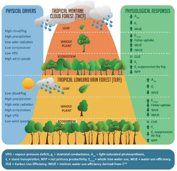
in these trees are lower than in lowland rainforest trees. Moreover, trees in TMCF tend to have higher water-use efficiency (WUE) and lose less water through transpiration (Hamilton et al., 1995; Rosado et al., 2016). In addition, the leaves of some tree species are capable of intercepting cloud water, an important feature known as "cloud stripping" (Figure 2.3) (Bruijnzeel and Proctor, 1995).

Figure 2.3: A comparison of the environmental drivers in tropical montane cloud forest (TMCF)

versus tropical lowland rain forest. The physiological responses of the vegetation at leaf, whole plant and ecosystem level are depicted for both types of tropical forests. Figure adopted from Gotsch et al. (2016).

(18)

2.2 Impact of global change on tropical montane

forests

Forests face multiple threats of anthropogenic origin. Many uncertainties remain as to how forests will respond to the combined pressure of deforestation, forest degradation and climate change in the long-term. This section elaborates upon the nature of these pressures and looks forward to what the future might hold for tropical montane forests.

2.2.1 Deforestation and forest degradation

Forests, especially tropical forests, are subjected to rapid deforestation rates. The area of land covered by forests has decreased dramatically over the last decades. In the period be-tween 1990 and 2015 approximately three percent of the world’s total forest area was lost (Keenan et al., 2015). Deforestation rates have been slowing down over recent years but remain nonetheless disturbingly high, especially in tropical countries (Table 2.1) (Keenan et al., 2015; FAO and UNEP, 2020). Historically, Andean cloud forests occupied ≈ 60 000

km2, but more than half of this area has been cleared over time (Mulligan, 2010).

The main driver for deforestation in Latin America is agriculture, both on commercial and local scale (Hosonuma et al., 2012). In Ecuador land use changes for human settlements and pasture have resulted in heavy deforestation of the Andean cloud forests (Wunder, 1996). Nowadays fragmented patches of TMCF or varying sizes can be found throughout a landscape matrix of other land uses (Scatena et al., 2010). By no means does this imply that remaining patches are in pristine condition, because in certain areas timber logging causes latent degradation of the forest ecosystem (Hosonuma et al., 2012). The extreme topography associated with tropical montane forests has provided temporary salvation for the remnant patches so far. Their limited accessibility and low population density resulted in a lower fragmentation than in tropical lowland forests (FAO and UNEP, 2020). However, the effects of climate change lie just around the corner. . .

Table 2.1: Trends in natural forest area. Forest area per region per year in 106_{ha (FAO, 2015).}

Region 1990 2000 2005 2010 2015

Ecuador 14.6 13.7 13.3 12.9 12.5

Neotropics 957.8 914.3 890.8 873.1 862.3

(19)

2.2.2 Climate change

Forests play a vital role in the global carbon cycle, because they act as a net carbon sink,

storing (2.4 ± 0.4) × 1015g carbon per year (Pan et al., 2011). This allows them to partially

buffer the increase in atmospheric CO2. However, the natural buffer capacity of the world’s

oceans and forests to store CO2cannot keep up with the rate at which this greenhouse gas

is being emitted. The atmospheric CO2 concentration has now reached a staggering 414

ppm (Tans and Keeling (2020)). As a result of this rise, 2019 was the second warmest year in a 140-year record and was marked by extreme precipitation and drought events across the world (NOAA National Centers for Environmental Information, 2020). Forests suffer from these changes: carbon stocks are sensitive to the daytime maximum temperature and precipitation in the driest quarter (Sullivan et al., 2020). Higher temperatures and more intensive droughts cause increased tree mortality in Amazonia, which results in a lowered capacity to store carbon. Indeed, carbon sink strength of these tropical forests appears to have declined since the 1990s (Hubau et al., 2020).

What exact impact climate change will have on tropical montane forests is still unclear; however, it is very likely that these forests will be hit harder than lowland forests. Montane ecosystems are thought to be more vulnerable to climate change and are likely to be the first regions to be affected by it. Tropical montane forests, for example, harbour many endemic species with narrow geographic and thermal ranges, which therefore face a high risk of extinction (Perez et al., 2016; Hill et al., 2019). TMF can therefore be regarded as an “early indicator of climate change" (Spehn et al., 2006).

The projected changes in atmospheric conditions will lead to an increased evaporative de-mand. This may affect the water cycle of the ecosystem through increased water losses by evapotranspiration (Gotsch et al., 2016). One could argue that the increased

atmo-spheric CO2 concentration might positively affect photosynthetic rates and lead to a higher

WUE and ecosystem productivity (Franks et al., 2013). However, warming-induced drought

stress is expected to dampen this CO2 fertilization effect through increased tree

mortal-ity in lowland as well as in altitudinal forests (Gómez-Guerrero et al., 2013; Hubau et al., 2020). Moreover, Bauters et al. (2020) found evidence for a decrease in intrinsic water-use efficiency (iWUE) in trees of the Congo basin cawater-used by rising temperatures over the

course of decades, countering the expected increase in iWUE as a consequence of the CO2

fertilization effect.

2.2.3 Ecosystem response

As stated in the previous sections, climate change is expected to have a profound impact on tropical montane forests. We differentiate between the short-term effects and long-term effects climate change will have on TMF (Figure 2.4).

(20)

survive despite high average regional temperature changes. On the other hand, species experiencing intolerable microclimatic extremes can go locally extinct in spite of moderate background climate change (Suggitt et al., 2011). The response of tropical forests to cli-mate change remains understudied in comparison with the response of boreal or temperate forests (Feeley et al., 2015).

A straightforward approach to detect upward species migration is to study changes in al-titudinal distribution of mountain vegetation over time. Moret et al. (2019) resurveyed the vegatation on Mt. Antisana, Ecuador and compared with Alexander von Humboldt’s

Tableau Physique _{denoting the altitudinal ranges of Mt. Antisana’s vegetation in beginning}

of the 19th century. The comparison revealed an altitudinal shift of ≈ 250 meters over

215 years. These upward elevational shifts provide insight into the speed at which climate warming affects the vegetation in mountain ecosystems (Steinbauer et al., 2018). The examined species did not respond uniformly to warming with some being able to follow cli-mate change rates and others lagging behind (Moret et al., 2019). This type of comparative studies is rather rare because it requires a time series of accurate species distribution data. Therefore this approach is not widely applicable in the tropics (Feeley et al., 2015).

The aforementioned method is insufficiently applicable. There is a need for alternative ap-proaches based on more-readily available data. Apap-proaches based on taxonomic or func-tional changes in a tree community offers an alternative for estimating the response of montane forests to climate change (Steinbauer et al., 2018). Prior to the immigration of species from lower-lying altitudes, abundances of the locally present species will shift to-wards a greater abundance of species able to tolerate the temperature rise (Smith et al., 2009). Hence, focusing on shifting species abundances provides an opportunity for esti-mating the response of ecosystems to climate change within a shorter timeframe than the one used by Moret et al. (2019) in their study on species migration.

Fadrique et al. (2018) conducted one of the few available studies on the response of trop-ical Andean forests to climate change, using an approach based on the thermal optima of tree species. This study encountered evidence for a directional shift in species composi-tion and relative species abundances in Andean forests over time. Species composicomposi-tion has shifted towards higher relative abundances of species from lower, warmer elevations, a phenomenon known as thermophilization (Gottfried et al., 2012). This trend is widely observed throughout Andean montane forests, yet the rate of compositional change varies across elevations (Fadrique et al., 2018).

The variation in compositional change rates can be explained by various factors. First, warming rates are not uniform but vary on a local scale. Microclimate can weaken or strengthen the impact of the background warming rate (Suggitt et al., 2011). Second, eco-tones like the cloud formation zone pose a barrier to species migration. The cloud-base ecotone plays a pivotal role in determining several microclimatic variables such as temper-ature, precipitation, light availability (Rapp and Silman, 2012; Letts and Mulligan, 2005). Tree communities around ecotones are dominated by specialist species. TMCF falls into this category of specialised tree communities. It may be harder for non-specialised species of lower altitudes to colonise these ecotonal forests and equally hard for specialist species to colonise zones higher uphill, further away from the ecotone (Foster, 2001). Third,

(21)

ther-mophilization rates can be limited by biotic interactions. Belowground linkages between plants and soil (a)biota may partially explain why mountain vegetation lags behind climate warming rates (Hagedorn et al., 2019). To predict how tropical forests will respond to cli-mate change in the long term, it is of key importance gain a better understanding of how environmental controls influence their ecological functioning (Aparecido et al., 2018).

Figure 2.4: Expected short- and long-term impacts of climate change on TMCF. Figure was edited

from Hagedorn et al. (2019) and contains general information on the impact of climate change on all mountain ecosystems (Hagedorn et al., 2019), as well as specific additional information on the expected impact on TMCF (Hubau et al., 2020; Suggitt et al., 2011).

The unusually high concentration of endemic species found in TMCF is the consequence of interlinked factors. The steep topographic gradients in mountainous regions give rise to a small-scale mosaic of different habitats in which the upper limit of lowland tree species and lower limit of montane species creates a species-rich interface. Together with the additional moisture gradient caused by the transition from humid lowlands to the drier interandean highlands, these factors gave rise to an explosive speciation, resulting in an unseen number of endemic species (Gentry, 1992; Foster, 2001; Homeier et al., 2010).

(22)

2.3 Elevational transect studies

In ecosystem research, elevational transects provide a unique opportunity to quantify long-term ecosystem shifts as a response to changes in environmental conditions (Malhi et al., 2010). Altitudinal gradients can be regarded as "space-for-time" substitutions when trying to understand the impact of climate change on ecosystems (Hagedorn et al., 2019). The underlying assumption is that the spatial differences between ecosystems along an eleva-tional transect are the result of long-term adaptation to the local conditions (Humboldt and Bonpland, 1805).

The steep environmental gradients over a short spatial distance represent an exciting re-search opportunity, because many environmental factors change while ascending a moun-tain. The most unambiguous shift with increasing altitude is a decrease in air temperature. Per kilometer gain in altitude the average air temperature drops by ≈ 5.5°C (Barry, 1981). Atmospheric pressure also declines with altitude. One could argue that the decrease in partial pressure of carbon dioxide reduces photosynthesis at higher altitudes (Gale, 1972). However, an increased carboxylation capacity and adapted leaf structure might partially counteract this phenomenon (Cordell et al., 1998). Under cloudless skies both radiation and the fraction of UV-B light are higher at high altitudes (Körner, 2007). It is difficult to generalise radiation patterns in TMCF along altitudinal gradients because clouds alter light quantity and quality (Reinhardt et al., 2010). Other environmental variables like relative humidity, precipitation and wind velocity may or may not increase with altitude depending on the region.

The shifts in environmental gradients when ascending a mountain are similar to the pat-terns observed with increasing latitude. However, setting up elevational transect studies in the tropics has the advantage of a lack of seasonal changes, which do have to be taken into account in large-scale latitudinal transects (Körner, 2007). Despite the existing knowledge on shifting physical drivers with altitude, it remains hard to distil a general altitude-related trend in biological phenomena such as productivity or plant functional traits. Distinct geo-physical drivers covary along a single altitudinal transect, and therefore it is difficult to attribute perceived trends to a single environmental variable (Körner, 2007).

Although caution is advised when interpreting the results obtained through an elevational transect study, this experimental set-up still provides unique opportunities to study the effect of environmental factors on plant morphology, speciation, physiological responses and ecosystem functioning.

(23)

2.4 Functional traits

Our study site is located in the Biodiversity Hotspot of western Ecuador. Approximately 9000 plant species can be found here, of which 25% are endemic to this region (Myers et al., 2000). Ecologists that are trying to make sense of this wide diversity and understand the driving mechanisms behind it, are increasingly focusing on an approach based on plant functional traits instead of taxonomy (Levine, 2016). Plant functional traits are defined as the ’morphological, anatomical, physiological, biochemical and phenological characteristics

of plants’_{(Violle et al., 2007). They are linked to the ecological strategy of a plant and can}

be defined at the level of an individual organ (leaf, stem) or at whole-plant level (Levine, 2016; Violle et al., 2007). An example of such a functional trait is adult plant height. This trait corresponds with a plant’s ability to capture light and disperse its seeds, but these ben-efits come at a construction and maintenance cost (Falster and Westoby, 2003). The plant realm is filled with these so-called ecological trade-offs, many of which can be quantified by means of functional traits.

The popularity of trait-based research has skyrocketed over the last two decades, resulting in an improved availability of plant trait data. The TRY initiative was founded in 2007 as an attempt to compile a global plant trait database (Kattge et al., 2011). As of July 2019, the TRY database comprised over 11.5 million trait records of 280,000 plant taxa for more than 2000 traits (Kattge et al., 2020). The existence of such vast databases has led to the construction of so-called Plant Economics Spectra.

2.4.1 Plant Economics Spectra

Ecologists discovered that only certain trait combinations are viable, implying a correlation between various traits. Hence, plants can be positioned along a reduced number of axes of variation. Throughout the last two decades, scientist have tried to capture these viable trait combinations in so-called spectra, reflecting ecological trade-offs. Wright et al. (2004) was the first to suggest the Leaf Economics Spectrum (LES): a framework in which leaf functional traits are positioned along one single axis, ranging from plants with a quick to slow return on investment. A detailed description of central leaf traits and their placement in the LES is available in Demol, M. (2016). When producing woody tissue, plants face similar trade-offs. Chave et al. (2009) considers wood density (WD) as a central trait in the framework of the Wood Economics Spectrum (WES). The axis ranging from low to high WD represents conflicting demands in terms of biomechanical support, water transport and storage of nutrients.

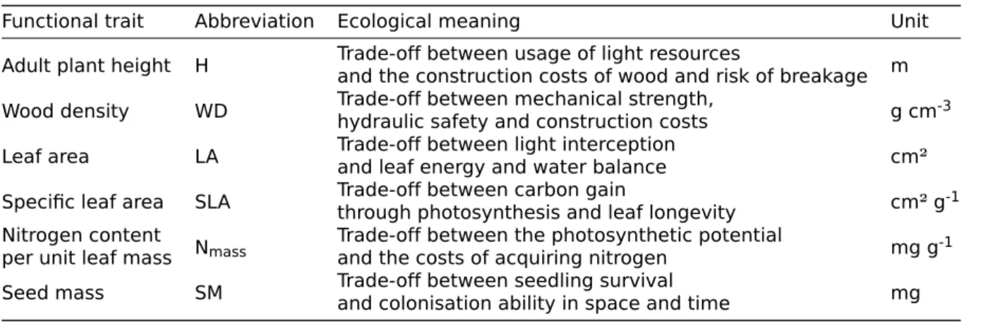
The spectrum of plant form and function as proposed by Díaz et al. (2016) was introduced as a two dimensional global spectrum with LES as one dimension and plant (organ) size as the second. Six traits are thought to capture the essence of plant form and function (Table 2.2).

(24)

Table 2.2: Six key functional traits according to Díaz et al. (2016) and commonly used

abbrevia-tions respectively. Their ecological meaning is briefly explained in terms of trade-offs. The unit of measurements used in this thesis are given for every functional trait.

Functional trait Abbreviation Ecological meaning Unit

Adult plant height H Trade-off between usage of light resources_{and the construction costs of wood and risk of breakage} m

Wood density WD Trade-off between mechanical strength,_{hydraulic safety and construction costs} g cm-3

Leaf area LA Trade-off between light interception_{and leaf energy and water balance} cm²

Specific leaf area SLA Trade-off between carbon gain_{through photosynthesis and leaf longevity} cm² g-1

Nitrogen content

per unit leaf mass Nmass

Trade-off between the photosynthetic potential

and the costs of acquiring nitrogen mg g-1

Seed mass SM Trade-off between seedling survival_{and colonisation ability in space and time} mg

The recent technological advancement in techniques such as airborne laser-guided hyper-spectral imaging or terrestrial laser scanning are opening up new perspectives for large-scale mapping of functional trait diversity (Asner et al., 2017b). Verbeeck et al. (2019) pleads for the construction of a Structural Economics Spectrum (SES) reflecting canopy structure properties from data obtained through terrestrial laser scanning. The incorpora-tion of SES, LES and WES could potentially lead to the creaincorpora-tion of a Global Plant Economics

Spectrum.

2.5 Functional diversity

The link between plant diversity and ecosystem functioning is not straightforward. The number of taxonomic tree species in a tropical forest does not necessarily determine its ecological functioning (Díaz, S. and Cabido, M., 2001). Moreover, species diversity in the tropics is often inadequately mapped (Feeley et al., 2015). To close the gap between tax-onomic diversity and ecosystem functioning, the concept of functional diversity (FD) was introduced. FD relates to the values and range of species functional traits. It correlates more strongly with ecosystem processes and ecosystem resilience to climate change than species richness does, hence the interest in quantifying FD through various metrics (Folke et al., 2004; Hooper et al., 2005).

We restrict ourselves to the use of four indices to quantify functional diversity within the scope of this thesis, each capturing a different aspect of FD: functional richness (FRic), functional evenness (FEve), functional divergence (FDiv) and functional dispersion (FDis). The former three indices were proposed by Mason et al. (2005) and further elaborated by Villéger et al. (2008), the latter was proposed by Laliberté and Legendre (2010). All four indices are independent and can handle relative abundances and multiple, continuous traits (Villéger et al., 2008; Laliberté and Legendre, 2010). The use of these indices results in a minimal loss of information, as opposed to dividing species into functional groups. Grouping species with continuous trait values into a discrete number of functional groups results in significant information loss (Wright et al., 2006).

(25)

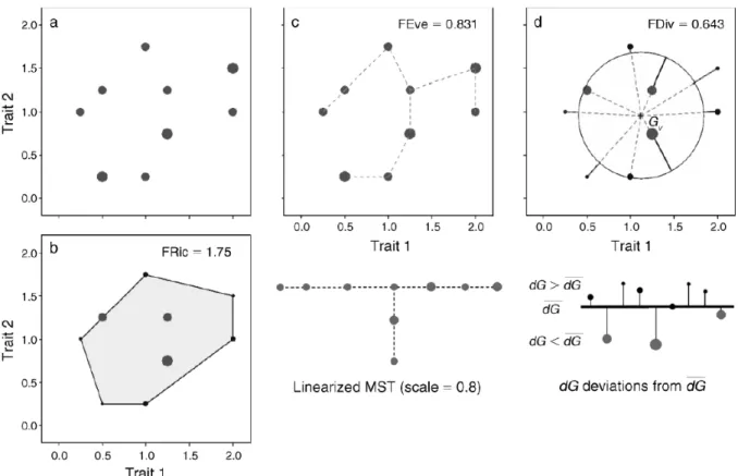
As visualised in figure 2.5, functional richness measures the amount the trait space oc-cupied by the species within a community (Mason et al., 2005). FRic is calculated as the minimum convex hull volume which includes all species and is a metric for habitat filtering. It is a measure for the whole of successful strategies among coexisting species in a certain environment (Cornwell et al., 2006).

Functional evenness can be computed as the counterpart of taxonomic evenness indices. FEve describes the uniformity of the distribution in the trait space and is calculated by means of a mimimum spanning tree. This is the tree linking all points in the trait space which minimises the sum of the branch lengths (Figure 2.5). FEve is maximal when the abundance of trait values in the trait space is uniform. A more uniform distribution of trait values could imply increased complementarity between species and result in a better use of resources (Mouillot et al., 2005).

Functional divergence captures to which degree the most abundant species occur at the extremities of the trait space. FDiv is calculated as the mean distance between the species and the trait space’s centre of gravity (Figure 2.5). If many abundant species lay far off-centred, FDiv will be high. A high value for FDiv indicates a high degree of niche differenti-ation, suggesting lower resource competition (Mason et al., 2005; Villéger et al., 2008). An additional FD index is called functional dispersion. FDis is the mean distance in the multidimensional trait space of individual species to the centroid of all species (Figure 2.6). FDis considers relative species abundances and is unaffected by the number of species in a community, which gives this metric an advantage over the aforementioned FD metrics (Laliberté and Legendre, 2010).

(26)

Figure 2.5: Summary of the calculation three functional diversity indices: functional richness (FRic),

functional evenness (FEve) and functional divergence (FDiv). (a) Representation of nine species within a two-dimensional trait space. The dots indicate the position of the species within the trait space according to their trait values. Dot size is proportional to species abundancy. (b) FRic is measured by the minimum convex hull volume including all inventoried species. In this example FRic is represented by the grey-coloured area. (c) The minimum spanning tree (MST) linking all species in the trait space is used as basis for calculating FEve. FEve measures the regularity of points and abundancies along the MST. The linearised MST is shown below panel c. (d) FDiv is measured as the mean distance

between species and the trait space’s centre of gravity (Gv), weighted by their abundance. Figure

adopted from Villéger et al. (2008).

Figure 2.6: Visualisation of the functional dispersion (FDis) calculation. Eight species are

repre-sented by dots in a two-dimensional trait space. The dot size is proportional to the relative species

abundancy. Vector c is the centroid of all species and zjis the distance of species j to centroid c. FDis

is calculated as the mean of all distances zj, weighted by the relative abundance ajof each species j.

(27)

2.6 Stable isotope compositions

In the 1930s, it was discovered that stable isotopes, including13_{C and}15_{N, are abundant in}

the natural world. Their natural abundance can be expressed as a ratio, standardizing for the natural abundancy of the stable isotope in a reference material. The reference materials

used in this study are Vienna Pee Dee Belemnite and atmospheric N2 for determination of

the stable carbon and nitrogen isotope composition respectively. The formulas used for the calculation of the stable isotope composition of a given sample are:

δ13C= ( 13_{C /} 12_C)_smpe (13_{C /} 12_C)_{reƒ erence} − 1 δ15N= ( 15_{N /} 14_N)_smpe (15_{N /} 14_N)_{reƒ erence} − 1

Natural abundances of the stable carbon and nitrogen isotopes can be used to assess

bio-geochemical and ecological processes. The drivers behind δ13C and δ15N have been

in-tensively studied over the last couple of decades. The photosynthetic pathway exerts an

important influence on the δ13_{C found in leafy tissue. Three major groups of plants with}

distinct photosynthetic pathways are being distinguished: C3, C4 and CAM (Crassulacean Acid Metabolism) plants. C3 plants include, among others, all arborescent life forms and use RuBisCo (ribulose biphosphate carboxylase oxygenase) as their most prominent carbon fixating enzyme in the Calvin cycle. RuBisCo discriminates against the heavy carbon iso-tope. PEP (phosphoenolpyruvate) carboxylase, the most prominent carbon fixating enzyme in C4 plants, exhibits this discrimination to a much lower extent (Farquhar, 1983).

The C3 pathway operates in ≈ 85% of all plant species, including tropical trees (Ehleringer et al., 1997). Other factors besides the plant’s photosynthetic machinery influence carbon

isotope discrimination. δ13C is also influenced by the ratio of intercellular versus ambient

partial pressures of CO2, soil moisture levels, temperature, light regimes and precipitation,

among other factors. All of these environmental factors act upon the stomatal conductance

and the CO2 assimilation rate of the leaf (Farquhar et al., 1989a; Körner et al., 1991).

Water is lost through the stomata during photosynthesis, hence a correlation exists between

δ13C and the intrinsic water-use efficiency of the plant (Farquhar and Richards, 1984). The

less negative δ13C, the greater iWUE (Farquhar et al., 1989b). The combined influence of

environmental factors may explain why δ13C increases with rising altitude (Körner et al.,

1991). This trend seems to depend on the plant life form as well. The effect of altitude on

δ13_{C for example seems more pronounced in trees than in lianas (Meeussen, C., 2017).}

Foliar nitrogen isotope ratios (δ15N) can provide insights into the nitrogen cycling across

ecosystems. δ15N is negatively correlated with mean annual precipitation (MAP) and

pos-itively correlated with mean annual temperature (MAT) and nitrogen availability (Craine

(28)

dicates a shift toward more nitrogen-conservative species at higher altitudes in ecosystems with a more conservative nitrogen cycle.

(29)

MATERIALS AND METHODS

In this chapter, the geographical and environmental characteristics of the study site are discussed, followed by a description of the protocol employed for remeasurement of plots. Hereafter the procedure for sampling leaf and wood specimens and their analysis is ex-plained. Finally, we discuss the statistical processing of the obtained data.

3.1 Study area

Seven clusters of reforested permanent sample plots (PSPs) in different altitudinal strata were established by Bauters, M. (2013). These PSPs are located in northern Ecuador on the western Andean flank in the provinces of Pichincha and Imbabura (Figure 3.1). Earlier work by Bauters, M. (2013); Bruneel, S. (2016); Demol, M. (2016) aimed to delineate undisturbed forest at the same altitudes, with the purpose of comparing the reforested sites with the natural climax situation in terms of carbon storage and functional diversity. In 2018, the first resurvey of the PSPs in natural forest was done by the botanist Nicanor Mejía. This resurvey took place in close cooperation with professor Selene Báez, affiliated with Escuela Politécnica Nacional in Quito. In 2019, our team conducted a second resurvey (Table 3.1). Each cluster consists of at least three square forest plots with a dimension of 40 by 40 m. The square shape has a lower edge:area ratio than other shapes, this results in less decision problems concerning edge trees than for rectangular PSPs (Phillips et al., 2002). Every plot was subdivided into four subplots of 20 by 20 m. The plot size of 0.16 ha is smaller than the recommended 1 ha by RAINFOR, but has proven to be more feasible in the scope of this research project (Bauters, M., 2013). Multiple smaller plots are more suitable for this study given the steep slopes in TMCF and the smaller chance to include human disturbances. Indicators of human disturbance are among others trails, logged trees and cattle tracks. The study features forest ecosystems along a 2800 m elevation gradient. Across this sect, clusters of PSPs at five altitudinal strata were delineated. The lower limit of the tran-sect comprises tropical lowland rainforest (stratum 1), the intermediate strata (strata 2, 3 and 4) encompass TMCF and the upper stratum (stratum 5) features TMCF near the treeline. Higher up the vegetation shifts to páramo grasslands.

(30)

Stratum 1 - Río Silanche Bird Sanctuary This reserve comprises 100 ha of Chocó-lowland Rainforest at 400 m a.s.l., located in the province of Pichincha, Ecuador. It is owned by the Mindo Cloudforest Foundation (MCF), a local non-governmental organization with the mission of conserving biodiversity on the western Andean flank. The reserve is part of a bigger reserve network that is currently made up out of five individual reserves (Mindo Cloudforest Foundation, 2019b). The surrounding landscape matrix mainly consists out of farmland for oil palm and cacao production (Meeussen, C., 2017). The most common tree species are Pourouma bicolor, Wettinia quinaria and Cecropia insignis. The high abundance of P. bicolor indicates that this reserve likely consists of secondary forest (G. Toasa, personal communication, August 2019).

Stratum 2 - Milpe Bird Sanctuary This 100-hectare reserve is also owned by MCF and

consists of Chocó-Andean foothills rainforest in the Pichincha province, at an elevation of 1100 m a.s.l. The Milpe and Río Silanche Bird Sanctuaries are home to an incredible amount of endemic birds, like the iconic Chocó toucan (Mindo Cloudforest Foundation, 2019a). This stratum has the highest tree species diversity. The most common tree species are Otoba

gordoniifolia_{, Stephanopodium angulatum and Ocotea sp.}

Stratum 3 - Maquipucuna Cloud Forest Reserve The PSPs in the Maquipucuna Cloud

Forest Reserve were set up at an elevation of 1900 m a.s.l. in the centre of the 6500-hectare reserve. Their remote location and closed canopy suggests the ecosystem here is truly primary cloud forest (Demol, M., 2016; Bruneel, S., 2016). A well-known inhabitant of this protected area is the Andean spectacled bear (Tremarctor ornatus) (Maquipucuna Reserve, 2019). Stylogyne ambigua, Cyathea caracasana and Cecropia herthae were the dominant tree species in this stratum.

Stratum 4 - El Cedral Ecological Reserve _{The ecological reserve El Cedral is located}

in Nanegal, near the valley of Yunguilla (Calacalí), Pichincha, Ecuador. It comprises 72 ha of primary cloud forest between 2200 m a.s.l. and 2500 m a.s.l. The surrounding landscape consists of natural forests. The owner of the reserve is Germán Toasa, a dedicated botanist who guided us during the field campaign in the summer of 2019. The most abundant tree species in this stratum are Beilschmiedia tovarensis, Chrysochlamys colombiana and

Weinmannia_sp.

Stratum 5 - Puranquí Community Forest _{The Puranquí Community Forest is located}

in the valley of Intag in the province of Imbabura. Four PSPs were established just below the tree line, at an altitude of 3200 m a.s.l. The forests in this region are threatened by bushfires (often lit on purpose) and illegal mining activities. Presence of grazing cattle was also noted near the PSPs. Given the close presence of the village and cattle, it is unlikely that the PSPs in this stratum comprise primary forest. Highly dominant tree species were

(31)

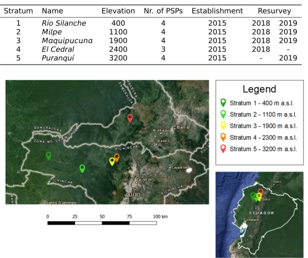
Table 3.1: General information on the strata established for this study. For each stratum the

eleva-tion in meters above sea level is displayed, as well as the number of permanent sample plots, the year of establishment and the years of remeasurement.

Stratum Name Elevation Nr. of PSPs Establishment Resurvey

1 Río Silanche ₄₀₀ ₄ ₂₀₁₅ ₂₀₁₈ ₂₀₁₉

2 Mpe ₁₁₀₀ ₄ ₂₀₁₅ ₂₀₁₈ ₂₀₁₉

3 Mqpcn ₁₉₀₀ ₄ ₂₀₁₅ ₂₀₁₈ ₂₀₁₉

4 El Cedral ₂₄₀₀ ₃ ₂₀₁₅ ₂₀₁₈

-5 Puranquí ₃₂₀₀ ₄ ₂₀₁₅ _- ₂₀₁₉

Figure 3.1: Location of the study sites. The right picture indicates that the strata can be found in

northern Ecuador on the western Andean flank. The location of the different strata is depicted on the left figure, showing that strata 1 to 4 are located in the province of Pichincha. Stratum 5 on the contrary is located in the province of Imbabura.

Table 3.2: Climatic characteristics include mean annual temperature (MAT), mean annual

precipita-tion (MAP), solar radiaprecipita-tion (E), water vapor pressure (Pw), average wind velocity (Vwind). Climatic data

with a resolution of 1 km2was retrieved from the WorldClim database version 2.1 (Fick and Hijmans,

2017).

Stratum 1 Stratum 2 Stratum 3 Stratum 4 Stratum 5

Latitude (N) 0.1473 0.0356 0.0968 0.1155 0.4497

Longitude (W) 79.1425 78.8665 78.6228 78.5724 78.4708

No. of PSPs 4 4 4 3 4

Plot size (ha) 0.16 0.16 0.16 0.36 0.16

Altitude (m a.s.l.) 394 - 420 1041 - 1098 1764 - 1953 2220 - 2521 3191 - 3241 MAT (°C) 23.8 20.0 17.6 15.9 11.0 MAP (mm) 3447 3050 1560 1391 1205 E (kJ m-2 day-1) 12051 13377 15518 15627 15716 Pw (kPa) 2.58 2.09 1.69 1.40 1.10 Vwind(m s-1) 1.28 1.60 1.94 2.31 2.70

(32)

The decline in mean annual temperature is strongly correlated with altitude. Many other

ecological drivers covary: mean annual precipitation and water vapor pressure (Pw) decline

with altitude, whereas wind velocity (Vwind) and incoming solar radiation (E)1increase. The

soil type for all strata is andisol (Bruneel, S., 2016).

3.2 Recensus of permanent sample plots

The methodology for this resurvey was based on the RAINFOR protocol (Phillips et al., 2002).

Delineating permanent sample plots

In the period of July to September 2019, the previously established PSPs were resurveyed. The GPS coordinates of previous field notes were used to navigate to the plot centre. The plot corners were marked with bright painted PVC tubes during the first resurvey in 2018. This was helpful during the delineation of the inner and outer plot borders. Attention was payed whether there were no tagged trees excluded or untagged trees included while stringing and whether trees near inner plot borders were included in the right subplot.

Tree tagging

Certain tree species reacted negatively to the nailing of numeration tags during previous field campaigns, so a fine, bright coloured rope was used to tie the tags to the trees instead. The tags were tied to the tree at a height of approximately 30 cm above the point of measurement (POM). New recruits with a diameter at breast height (DBH) larger than or equal to 10 cm were tagged. During every field campaign a distinct tag colour is used. Some trees had lost their tag over the years. In this case, the previous tag number was figured out based on information on diameter and tree species. Subsequently, these trees were given a new tag and the new tag number was carefully linked to the old. Trees that could not be found were assumed to be dead.

Diameter measurement and marking of trees

The standard POM was at a reference height of 1.3 m. To define the POM in the field, a pole marked at 1.3 m was pushed firmly into the soil at the downhill side of the tree. The reference height was measured as the straight-line distance along the trunk, not as the vertical height above the ground (Figure 3.2). Sometimes the POM differed from this reference height, in order to avoid deformities or buttresses. In this case, the height of the alternative POM was recorded. The POM was marked on the stem with bright spray paint. Certain special cases we handled as follows:

1_{Solar radiation (E) is assumed to increase with rising altitude. The values represented for E in Table 3.2 are} daily averages under the condition of cloudless skies. Given that cloud cover plays a central role in tropical montane cloud forests, the level of solar radiation actually reaching the forest floor may be altered strongly as a consequence of persistent cloud cover.

(33)

• The cambium of leafless trees was slashed to clarify whether these trees were still alive.

• Although the RAINFOR protocol advises to only tag the largest stem of multiple-stemmed trees, we tagged every stem and noted carefully which tag numbers belonged to the same tree. This approach leaves less room for discussion when comparing diameters between distinct resurveys.

• Since the survey of Bruneel, S. (2016) and Demol, M. (2016) pointed out that only four lianas with a DBH > 10 cm were present within the PSPs, their contribution to the overall carbon storage was considered as negligible in comparison to the contribution of trees. Hence, no liana diameters were measured. For more detailed info on lianas along the transect see Meeussen, C. (2017).

Figure 3.2: In certain cases, the reference height of 1.3 m cannot be used as the point of

measure-ment in order to avoid deformities. (a) In leaning trees, 1.3 m length is measured along the side of the stem closest to the ground. (b) If the tree is buttressed at 1.3 m, the stem is measured 50 cm above the top of the buttress. (c) The point of measurement is determined at the downhill side of trees on a slope. Adopted from Phillips et al. (2002).

Tree height measurement

The understory in nearly every stratum was very dense. Since the Nikon Forestry Pro uses a laser beam to measure tree height, its use is restricted to those trees with an uninterrupted view between the observer’s eye and the stem basis and between the observer’s eye and highest point of the tree’s crown. In practice, finding such trees was a highly time-consuming process. Therefore no tree heights were measured, instead DBH-height relation-ships determined in earlier work were used (Bauters, M., 2013; Bruneel, S., 2016; Demol, M., 2016).

Species identification

Trees were identified by the botanist Germán Toasa. To observe the leaves and flowers of a tagged tree, a camera with a powerful optical zoom was used. Fallen leaves, fruits or flowers and the smell of the slashed bark provided additional clues. When an individual could not be identified in the field, a botanical leaf sample was made to allow identification afterwards. In case the tree species could not be determined, the genus was recorded.

(34)

3.3 Leaf sampling and analysis

For every plot we composed a list of the cumulative basal area for all occurring tree species, ranked from most to least abundant. To get an accurate representation of leaf traits on plot level the most dominant tree species that make up a large proportion of the basal area were sampled. Tree species were ordered on the basis of the percentage of the basal area they represented on plot level. We aimed at sampling leaves of the most abundant tree species making up 80 % of the total basal area of each plot.

Leaf samples were collected with a telescopic tree pruner with a maximum length of twelve meter. If possible at least three individuals per species were sampled, preferably trees in different diameter classes. The collected leaves originate from the middle or the lower sections of the trees. It was not possible to collect sun leaves originating from a section of the tree higher than the length of the tree pruner. From each tree a sub-sample of five leaves within a range of different ages was taken (excluding juvenile, sick and dying leaves). The leaf samples were oven-dried at 70°C for at least 48h to avoid contamination by funghi.

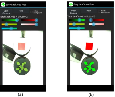
Leaf area (LA) was determined of fresh leaves with the aid of the application Easy Leaf Area, developed at Department of Plant Sciences of the University of California by Easlon and Bloom (2014). This is a free, open source software designed with the purpose of enabling rapid LA measurements in the field. LA can be determined by means of photographing the leaf with a red reference square of two by two cm (Figure 3.3). The LA is then calculated using the RGB value of each pixel to identify the leaf in each picture. The accuracy of this method is very high even with the common camera of a phone, but the user must be careful to avoid perspective and lens distortion (Easlon and Bloom, 2014). We determined the LA (petiole included) on the same day as the samples were collected using a smartphone camera. Directly after collecting the sampled leaves are the greenest. Over time they turn brown and shrink which makes it more difficult to distinguish the leaf pixels from the red scale pixels. The application Easy Leaf Area is able to process multiple leaves of one sample at a time. The cumulative LA of every sample was noted.

The dried leaf samples were weighed using a precision balance with a readability down to

0.1 g to obtain the cumulative dry weight (Mdry) of all leaves making up one leaf sample.

Specific Leaf Area (SLA) was calculated by dividing LA of all sampled leaves per individual by their summed Mdry: SLA =MLAdry.

After determining SLA, the samples were ground into a fine powder using a Retsch ZM-200 centrifugal mill at sieving pore diameter of 0.2 mm. Thereafter, all chemical analyses were conducted at the Isotope Bioscience Laboratory (ISOFYS) at Ghent University. To determine mass-based leaf nitrogen (LNC) and carbon content (LCC) 2.70-3.30 mg of each sample was analysed using an elemental analyser (Automated Nitrogen Carbon Analyser; ANCA-SL, SerCon, UK), interfaced with an isotope ratios mass spectrometer (IRMS; 20-20, SerCon, UK). In total, 260 leaf samples were sent for analyses of LCC, LNC, leaf nitrogen and carbon stable isotope composition.

(35)

Figure 3.3: Usage of the application Easy Leaf Area. (a) Tap ’Open Camera’ and take a picture of

the leaf and the red scale area. Both should be at the same distance from the camera and parallel to the camera. (b) By moving the sliders leaf and scale identification are adjusted and a value for the leaf area is obtained. Pixels identified as leaf pixels are recoloured pure green and scale pixels are recoloured pure red for visual confirmation (Easlon and Bloom, 2014). (Easy Leaf Area license Copyright © 2012, 2013, University of California. All rights reserved.)

3.4 Wood sampling and analysis

We collected wood samples of tree species that had not been sampled for wood during previous inventories. In total 59 wood samples covering 47 tree species were taken using an increment borer with a core diameter of 5.15 mm (Haglöf, Långsele, Sweden). All wood cores were taken at breast height (1.3 - 1.4 m) of trees standing outside of the PSPs. It is important to not damage the trees standing inside of the plot, because this might disturb natural mortality rates. We aimed for a drilling depth slightly longer than the tree’s radius. However, this drilling depth could not be achieved in individuals with very hard wood to avoid breaking the auger. We followed the instructions of Grissino-Mayer (2003) when coring the tree and extracting the core (Figure 3.4). If possible, multiple individuals of the same tree species were sampled so the variability of wood specific gravity between individuals could be determined. For 11 out of the 47 sampled tree species we were able to collect two or more samples. The wood cores were stored in paper straws and dried for 48h at a temperature of 103°C to drive off all free and bound water (Williamson and Wiemann, 2010).

Specific Gravity (Gb) of wood is an important ecological trait that is calculated as the oven

(36)

Figure 3.4: Instructions for collecting wood samples. (a) Place the tip of the borer in an angle of

90° at the appropriate boring height. Grasp the shaft of the auger with one hand and hold the handle center with the other. (b) Apply inward pressure to help the auger tip penetrate the outer bark. Keep applying this pressure while rotating the increment borer until the threads engage and the auger tip enters the tree. (c) Slide the extractor into the auger and turn the handles counter-clockwise for two turns. (d) Pull the extracor cap gently until the core breaks free (Grissino-Mayer, 2003). Figure adopted from Chave (2005).

Figure 3.5: Two methods for assessing the volume of increment cores. (a) Experimental set-up for

the water displacement method. The green volume of the wood core is measured by immersing the wood sample in a container of water. The volume of the sample is then equal to the weight of the

displaced water, since water has a density of 1 g/cm3 _{(Chave, 2005). Figure adopted from Hossain}

et al. (2017). (b) Our experimental set-up for determining wood density. (b.1) Mdry is determined

using a balance with a readability of 1 mg. (b.2) Wood samples are submersed in water for 48 h. The

rehydrated wood core has a volume that is not significantly different than the original Vgreen(Schüller

et al., 2013). (b.3) The length of the rehydrated wood core is measured geometrically with a digital caliper.

Mdrywas determined using a balance with a readability of 1 mg. A frequently used method

to determine Vgreenof wood cores is the water displacement method (Figure 3.5). However,

we chose to measure Vgreengeometrically instead of using the water displacement method.

The reason for this is the fact that the wood cores shrink significantly after extraction in

both in the radial and axial direction, which results in a biased Gbmeasurement when using

the water displacement method (Schüller et al., 2013). The alternative is measuring the length of a rehydrated wood sample geometrically with a digital caliper (Figure 3.5). This measurement is a good approximation for the length of the freshly collected wood sample. The green volume is calculated using this length and the uniform sample diameter of 5.15 mm (identical to the diameter of the increment borer). Green volumes calculated in this way are believed to be a more reliable approximation of the true green volume (Schüller et al., 2013). Finally, we acknowledge that wood density varies from in radial and axial direction, but did not account for this variation, nor did we account for compaction caused by the auger tip.

(37)

3.5 Statistical analysis

The data analysis was performed using R (version 3.6.3), an open source software pro-gramme (RStudio Team, 2019).

3.5.1 Taxonomic diversity

All plant species names were standardised with the aid of the R package taxonstand (Cayuela et al., 2019). Taxonomic authorities for all species referred to in this thesis are available from the Plant List (www.theplantlist.org).

Five taxonomic diversity metrics were calculated to assess the species richness and com-position of permanent sample plots using the R package vegan: species richness, rarefied species richness, Shannon diversity index, Simpson diversity index and Pielou’s evenness index (Oksanen et al., 2019; Shannon and Weaver, 1963; Simpson, 1949; Pielou, 1966). The comparison of species richness between plots of different dimensions is misleading, as this measurement does not take into account the larger number of observed trees asso-ciated with the altered plot size. Rarefaction methods standardise species richness for a given sample size and facilitate the comparison of species richness between plots in differ-ent strata. In this master thesis, the rarefied species richness was calculated for every plot using the lowest observed stem density (47, stratum 1 plot 4) (Gotelli and Colwell, 2001). To compare the floristic composition the pairwise Bray-Curtis dissimilarity between strata was calculated (Bray and Curtis, 1957). The general formula for calculating the Bray-Curtis dissimilarity between stratum x and y is as follows:

BCy= PJ j=1|nj− nyj| PJ j=1nj+ nyj (3.1)

with nj the number of counts for species j in stratum . This measure takes on values

between 0 (completely identical strata) and 1 (completely disjoint strata). The contribution of species j to the overall dissimilarity is weighted by its relative abundance. Because the computation involves summing the absolute difference between species counts, an under-lying assumption of the Bray-Curtis measure is that the strata have an equal sample size. This is not the case in our dataset so the dissimilarity between strata was overestimated due to the fact that a part of the difference between two strata can be explained by the difference in sample size (Ricotta and Podani, 2017).