PBL-report
Struggling to deal with
uncertainties
What is known about indirect
land-use change?
Anne Gerdien Prins, Koen Overmars and Jan Ros AnneGerdien.Prins@pbl.nl
November 2014
2
Summary
Modelling approaches in literature show a wide range of emissions from indirect land-use change (ILUC), which can be traced back to several assumptions, implicitly made within the model structure or parameters. Several analyses show the sensitivity of the calculated ILUC or ILUC emissions to the uncertainties in the models. It is not realistic to assume that these uncertainties can be reduced, considerably, in the coming years. However, all modelling results, together, do point to the risk of ILUC effects caused by biofuels based on agricultural products. Capping the use of food crops in the EU Renewable Energy and Fuel Quality Directives seems an appropriate way to limit the risk of emissions from indirect land-use change, at least in the short term.
This paper shows the efforts that would be required to achieve a maximum ILUC emission level of 21 gr CO2/MJ, for a range of crops and final land conversion emission factors. These efforts concern
compensating mechanisms, such as yield increases and consumption diversions. The data indicate that, for the amount of biofuel needed to reach the blending target, achieving this level of ILUC emissions cannot be taken for granted, even in the case of land conversion with relatively low conversion emission levels.
1. Introduction
In 2008, sustainability criteria for biofuels were presented, at the time of the adoption of the Renewable Energy Directive (RED; (EU, 2009a)) and revision of the Fuel Quality Directive (FQD; (EU, 2009b)). However, the criteria did not include indirect land-use change (ILUC) – an important sustainability issue. Warnings of potentially severe impacts could already be heard at that time. Therefore, the Commission proposed that criteria for ILUC would be added, following additional research on the issue. The European Parliament and Council requested the Commission to propose policy options for managing ILUC, by 2010.
Since 2008, several studies and reviews have been published that identify ILUC and indicate the various orders of magnitude ((Edwards et al., 2010; Prins et al., 2010; Overmars et al., 2011; Wicke et al., 2012) ), including an impact assessment for the European Commission (Laborde, 2011). Review results show that it is difficult to draw conclusions on the exact height of the expected ILUC emissions per crop. Particularly, because a large part of the variance in outcomes originates from differences in assumptions in model structures and chosen parameters. However, they do confirm the potentially serious impact. The range of outcomes demonstrates ILUC could undo the expected emission gains of biofuels. Also, the study by (Overmars et al., 2011) on the ILUC effects of biofuels used in the past, which uses as many monitoring data as possible, shows that differences in assumptions on ILUC emissions range from around zero to twice the fossil fuel emissions.
So far, no political agreement has been reached about criteria to prevent unsustainable ILUC effects. The proposal of the European Commission in 2012 included a cap of 5% on biofuels produced from food crops and a reporting obligation of estimated ILUC. A cap of 5%, which is about the current level of agricultural product use, would probably minimise the ILUC effect. In the meantime, the European Parliament proposed a cap of 6% and, recently, the European Council agreed on a cap of 7%,
3
greenhouse gas emission balances were used, particularly with the argument that these factors are too uncertain. They only play a part in the proposal of the Commission on reporting by using ILUC factors per crop group derived from the impact assessment (Laborde, 2011).
The level of uncertainty compared to the presumed emission benefits clearly shows the need to include ILUC in existing policies. However, the ‘indirect’ nature of ILUC makes the debate far from straightforward and influenced by a large variety of interests. One of the arguments against using these emission factors is that scientific evidence should be improved before ILUC effects or emission factors could be taken into account in criteria or regulations. However, uncertainties will probably remain, implying a remaining risk – not a certainty – of more CO2 emissions from using biofuels
instead of the fossil alternative. Therefore, biofuel and/or ILUC policies should be based on risk management. The cap of 5% on biofuels from food crops in the current EC proposal, for example, can be seen as a type of risk management.
The current sustainability discussion on biofuels strongly focuses on emissions per unit of energy, while several other relevant sustainability issues have been marginalised. The important basic question in the sustainability assessment of biofuels is:
What is considered sustainable, in relation to biofuels and the related land use?
Do we take into account only greenhouse gas emissions, or also impacts on biodiversity and food security? Do we assess only the biofuel chain and its direct impacts, or also the land-use-related impact or even the full impact of the use of biofuels? If so, then we also have to include the indirect impacts. If we would be precise about what is considered sustainable and what is unsustainable regarding the (in)direct effects, it would be helpful for selecting the assessment method(s). To assess the biofuel chain, a life-cycle analysis would be sufficient. For analysing any indirect effects, global models may be needed. Assigning indirect impacts of biofuel use to a specific biofuel chain would increase the uncertainties involved.
At this moment, a definition of what is regarded sustainable is not available and, therefore, there are many questions with a host of different answers. A few examples:
• Are all impacts on food consumption unsustainable? Which changes are considered unsustainable and which acceptable? To what extent is a decreasing demand for food and feed acceptable, and should we make a difference between food prices in developing countries and feed prices in developed countries?
• Is any loss of biodiversity due to biofuel production unacceptable? Should short-term land conversion and long-term climate impacts be included? Or should a minimum area size be ‘reserved’ for nature in a future, sustainable world?
• Regarding the potential use of unproductive land: is growth or regrowth of natural
vegetation the alternative? This natural vegetation could take up more CO2 – estimated at 0
to 16 tonnes CO2/year (Searchinger et al., 2008a) – and store it for a longer period,
4
Box 1. What is indirect land-use change?
Indirect land-use change (ILUC) is the phenomenon that occurs when crops are being diverted to other cropland due to an increased demand for biofuels. Biofuel targets or blending mandates increase the demand for biofuel, and thus for biofuel crops. Currently, particularly food and feed crops are used, such as maize, wheat and sugar cane. The cultivation of these crops requires
additional land. Sustainability criteria prohibit the cultivation of biofuel crops in forests and on highly biodiverse grasslands. The crops can be grown on unproductive land or currently managed land (Figure 1). In case of the latter, the agricultural crop formerly produced on that land must be diverted to elsewhere, or the consumption level of that particular commodity should decrease. Growing these crops somewhere else means either intensification of crop farming on existing agricultural land, or taking non-agricultural land into production. This is called indirect land-use change (ILUC). The conversion of land with natural vegetation to cropland causes emissions – the so-called ILUC emissions.
The first part of this paper explains why uncertainties cannot be excluded from the assessment of ILUC effects and which parameters are especially responsible for these uncertainties. The second part indicates the required efforts to keep ILUC emissions at an acceptable level.
5
2. Uncertainties in ILUC calculations
Using assumptions in ILUC calculations is inevitable
The ranges in ILUC emissions resulting from model calculations particularly reflect the indirect nature of land-use change and its complexity. The impacts of biofuel production vary: from intensification to consumption change to land conversion (see box 1). The ratio between those effects is barely known and probably not constant towards the future or in the context of other – constraining –
circumstances. Moreover, measuring impacts at the end of the causal chain is not possible, since the final impacts of biofuel policies cannot be distinguished from those of other developments.
Therefore, many assumptions are involved in determining ILUC impacts. There are three different types of assumptions that have a large effect on sustainability assessments of biofuels, which follow from the basic assumption or definition about when biofuels can be considered sustainable:
1. What would have happened in a world without biofuels; in other words, what is the reference? 2. What processes should be taken into account; what are the system boundaries? This defines the
choice of calculation method. Choosing an existing model implicitly defines the system boundaries.
3. What assumptions are already included in the calculation method or model? This concerns the parameters within a particular model that define relationships.
The following section elaborates on the uncertainties, but first the steps needed to calculate ILUC emissions per unit of energy are discussed below. The schematic clarifies the role of each assumption within the calculation.
Calculating ILUC
The calculation of ILUC emission per unit of energy can be divided into three steps (Figure 2). Firstly, the agricultural yield level and industrial processing efficiency of a given crop define the gross area needed to grow enough product for one unit (megajoule) of biofuel. Secondly, the actual use of by-products, diversion of other uses, intensification of agricultural production, land expansion and trade, which are all indirect effects, determine the net area needed to produce this unit of biofuel. The last factor to determine the ILUC emissions per unit of biofuel are the emissions related to the possible conversion of land needed.
6
Emissions due to intensification of agriculture are not included in this scheme.
The reference world
To assess biofuels on their sustainability, one needs to define what happens in a world without biofuels (or without biofuel policies). Different assumptions in the reference scenario cause differences in calculated ILUC emissions. The main assumptions are about:
1. Developments in the demand for food and feed, based on dynamics of population, economy and diet;
2. Developments in the price of crude oil;
3. Developments in the types of passenger vehicles used, which in turn determine the demand for bio-ethanol or biodiesel;
4. Developments in agricultural technology due to current and future research and innovation, particularly regarding new breeds and varieties, which result in yield increases or changes in the ratio between feed product and biofuel product ;
5. Developments in technologies to convert biomass into fuel, including the refining of biomass into specific products;
6. Developments in policies, especially on trade, agriculture and spatial planning; 7. The amount of regrowth, with respect to the CO2 uptake at abandoned fields. This
determines the foregone CO2 uptake in case biofuel crops are grown on these fields.
These assumptions, together, for example, determine the developments in agriculture, such as the regions of the world in which agricultural area will decrease, and those with increased production or expansion. ILUC in regions with a decrease in agricultural area causes lower emission levels than in regions of agricultural expansion. In the absence of dedicated biofuel policy, oil prices strongly affect the amount of oil that will be replaced by biofuels, and, therefore, also the amount of biofuel needed
7
for achieving the biofuel policy target. The amount of biofuel used to voluntarily replace oil, thus, partially determines the level of policy impact.
Model choice
Most of the ILUC factors are calculated by a modelling approach, since that allows for separation of the impacts of biofuel policies. In such an approach, two scenarios are analysed; one expressing the reference world (the reference scenario), and one including the biofuel policies. Subtracting the first scenario outcome from the second results in the indirect land use or other indirect impacts from biofuel policies.
The model chosen, in part, determines the outcome, because many assumptions are implicit in the model structure or model parameters. The model, for example, determines the processes that are taken into account, such as the impacts on trade, food security and carbon uptake, and the detail of spatial variation. Another important model characteristic is where it looks for a solution; Computable General Equilibrium (CGE) models and Partial Equilibrium (PE) models, which have often been used for ILUC-calculations, look for a new equilibrium in the economy. While looking (iterating) for a new equilibrium, the model dilutes the impacts over the whole global economy. Although the dilution over the whole global economy occurs in reality, it may be a more bumpy process than CGE models suggest, since economic actors only react when prices are changing, and adaptations in the economy usually do not happen in advance.
Because a definition of the sustainability of biofuels has not been defined, all kinds of models have been used to calculate ILUC emissions. In that sense, the wide range of results is not surprising. Meanwhile, researchers are developing and expanding the models further. System boundaries can be stretched and new relationships can be taken into account. For example, the importance of land and by-products for feed, in the ILUC calculations, have led to an introduction or more detailed
representation of those aspects in several models, over the past few years. However, adding
relationships and more details also requires data to parameterise, but these are not always available. Therefore, adding more details or extending models often also adds to the degree of uncertainty about the results.
We elaborate on the specific uncertainties in processes modelled, such as the choices in model structure, below.
Uncertainties in model parameters
General and partial equilibrium models require hundreds of parameters, with many of which only loosely based on empirical data (Hertel et al., 2007). Parameter uncertainties vary; some data are based on monitoring, others are derived from monitoring data.
An important category of parameters is that of elasticities that express changes in the demand for goods due to price changes. Therefore, shifts can occur between consumed goods (e.g. shifts in diet), between production factors (e.g. capital, labour and land), or in intermediate input (e.g. maize or wheat as input for ethanol). Preferably, estimations of these elasticities should be based on data. However, the scientific base for the elasticities used seems small, especially since a derived elasticity heavily depends on the situation in a certain region over the observed period. For example, the choice to use more fertiliser to increase production instead of expand cultivated land depends on: 1) the current use of fertiliser, 2) management technologies available, and 3) social acceptance and
8
policies on fertiliser and agriculture, in general. Extrapolation of the, relatively few, literature-based elasticities to other regions or into the future is frequently practiced, because it is the best available data. However, often there is relatively little emphasis on the uncertainties involved.
Moreover, it is the relative size of the elasticities with respect to each other that matters (Keeney and Hertel, 2008; Golub and Hertel, 2011), i.e. the modelled reaction to changes in consumption versus intensification versus land expansion (see Figure 1). Especially for the impact of biofuel policies on emission levels, this relative size matters. Most reported calculations do not include emissions related to intensification of agriculture (e.g. from fertiliser use) or any negative impact of consumption change.
The largest part of the unknown uncertainty probably can be found in the second step of Figure 2. It describes the impact of biofuel policies on the economic system, and the responses of farmers, industries and services that use agricultural input, and end consumers. Plevin et al. (2010) show that this ratio varies between 0.2 and 0.8 in a range of reviewed modelling exercises for corn ethanol in the United States.
The parameters needed in the first step are either monitored or derived from practical processes. The uncertainty of those parameters is limited to variations with respect to the mean. The
parameters in the following steps, in contrast, are far more uncertain. Therefore, we elaborate on the major uncertainties of those parameters in the following sections, starting with the actual use of by-products.
Uncertainties about specific dynamics
Actual use of by-products
Including by-products in a model to assess ILUC is important, since they may replace products in markets than that of biofuel, and, therefore, not all land used for growing biofuel crops has to be attributed only to that biofuel crop. This decreases the net area needed. However, it is likely that not all biofuel crop by-products can replace the products formerly used for feed (therefore we
distinguish possible and actual use of by-products). Since by-product prices will be lower, due to a larger supply resulting from the biofuel mandate, consumption of by-products is likely to increase. In that case, the reduction in gross area will be smaller, as not all of the by-products will substitute former feed products. In reality, the average actual use of by-products depends on the price
response by farmers and the substitution possibilities. The last depends on the animal for which the feed is used, as well as on the ingredients in the byproduct in addition to its major component, such as protein. Whether physical units, such as tonnes of produced proteins, are used to substitute between products depends on the CGE model. If physical units are incorporated, major ingredients (e.g. protein) are often used as the basis (Laborde and Valin, 2012). However, proteins can differ in quality and cannot be assumed to automatically substitute each other. Awarding substitution values that are too generic, leads to overestimation of the end use of the particular by-product, and thus to underestimation of the net area required.
9
Example I: Laborde and Valin (2012) forced their model in such a way that no production of dried distillers grains with solubles (DDGS) – a byproduct of wheat ethanol –take place. This resulted in an ILUC factor of 41.6 gr CO2/MJ instead of the 38.6 gr CO2/MJ in the reference case. In another, similar
analysis the by-product of oilseed, meal, was not produced. This resulted in an ILUC factor of 45.2 gr CO2/MJ instead of 38.6 CO2/MJ. When the model was forced to produce neither meal from oilseed nor
DDGS from wheat, the ILUC factor increased to 48 gr CO2/MJ.
Example II: The analysis by Taheripour et al. (2010) showed that not including by-products in model calculations could overstate the land conversion by about 27%: harvested area of 15.6 Mha instead of 12.3 Mha, in 2015, to comply with EU and US biofuel policies. Their analysis also showed that food consumption could increase due to cheaper by-products. An analysis that included by-products and kept food consumption constant, compared to the reference case, resulted in an additional harvested area of 11.5 Mha.
Consumption change
The diversion of crops away from consumption or other uses can ‘provide’ biofuels without using extra land; it decreases net land use. Other by-product uses – besides for livestock feed (see above) – are in the form of resources for intermediate sectors that use the primary agricultural commodities as input to produce goods other than food or feed. Vegetable oil, for example, is used in many products (e.g. shampoos). In reality, such a diversion could mean that food becomes too expensive for the poorest people to buy, while more prosperous people may be willing to pay a higher price, but the amount of food they eat is the same as before. In CGE models changes in consumption are simulated using price elasticities of demand for agricultural output, and in some of these models those are adapted to income to reflect a changing diet at higher income levels; as prices decline, people will not eat ever increasing amounts of grain. This is modelled as Constant Difference of Elasticities, for example, in the models GTAP (Golub and Hertel, 2011) and MAGNET (Kavallari et al., 2014). However, calculating consumption on a physical basis, such as calories, is surprisingly absent from most models; therefore, modelled consumers can switch between different goods without any implication for their ‘physical’ diet (e.g calory intake). This means that, in reality, consumption may be more rigid than most CGEs project.
10
Example I: Hertel et al. (2010b) fixed the food consumption, which resulted in a 41% increase in ILUC emissions per MJ, compared to the reference scenario.
Example II: In the central NAP scenario of Laborde and Valin (2012), consumption diversion plays a dominant role; for most agricultural goods, around 50% or more of the required biofuel amount is provided by demand diversion. For wheat and maize, this is especially due to by-product use; for sugar, mainly due to the diversion of other demand; and for vegetable oil, around a third is due to end- use diversion, and two thirds to other demand diversion. Only for sunflower oil, 80% of the required biofuel amount has been provided by additional production. Keeping food consumption on the same level as under the reference scenario resulted in an 54% higher ILUC emission level per MJ. Keeping only crop consumption constant resulted in an increase of 52% of the ILUC emission level per MJ, whereas keeping meat consumption constant increased the ILUC emissions by only 2% (Laborde and Valin, 2012).
Intensification of agricultural land use
Several processes play a role in the intensification of agriculture, and all have their own dynamics and uncertainties. Therefore, we separated them into the categories below:
Yield increase due to changing management
This process is also called the intensive margin or the price-induced yield increase. The
argumentation is that when farm gate prices of commodities increase, farmers tend to use more input (fertiliser), more capital (investments) or labour per unit of land, with different substitution possibilities between the various inputs and endowments. Empirical evidence for the dynamics in substitution is partially and/or regionally available; for example, for US maize, as investigated in Keeney and Hertel (2008), and for EU agriculture, as was shown by Salhofer (2000) who reviewed several studies. In CGE models, the values available are often extrapolated or adapted to other regions in the world (Golub and Hertel, 2011; Laborde and Valin, 2012; Kavallari et al., 2014), because they are the best available. However, this dynamic is highly uncertain, especially with respect to a changing policy context or new technologies.
11
Example I: GTAP used to have a ‘yield response to price’ parameter of 0.25, which means that a permanent increase of 10% in crop price, relative to variable input prices, would result in 2.5% higher yields. Decreasing this parameter to 0.1 for all regions and all crops results in a 37% increase in additional cropland for 1Mtoe in biofuel, compared to the reference scenario (Golub and Hertel, 2011).
Example II: Kavallari et al. (2014) varied the substitution elasticity between land and fertiliser. This parameter defines the change in the ratio between land used and fertilizer applied, when the ratio between land and fertiliser price changes. The base scenario uses a value of 1.25. Decreasing this substitution elasticity to 0.15 – as used in Laborde (2011) – results in a 50% increase in additional cropland for 1 Mtoe in EU biofuels. Increasing this value to 2.7 (Salhofer, 2000) results in a 25% decrease in additional land used per ktoe of EU biofuels.
Example III: Kavallari et al. (2014) also varied the substitution elasticity between land and other endowments from the default 0.1 to 0.3, based on Salhofer (2000). This results in a 10% increase in additional land used per ktoe in EU biofuels.
Intensification of rotation
In certain regions, farmers rotate their crops to reduce pests, diseases or soil compaction. For example, the first year, they grow a certain cereal crop, followed by potatoes in the second year, again a cereal crop in year three, and sugar beets in year four, after which the rotation starts again from year one. In some regions, it is common practice to let a field lie fallow for a year, from the perspective of good agricultural practice, or induced by policies. On the one hand, abandoning the practice of the fallow year may increase production without the need for additional agricultural land. The drawbacks would be, for example, the foregone benefits of increasing soil carbon levels, or of carbon uptake in cases where fields lie fallow for more than one year. On the other hand, including fallow years in the rotations at fixed intervals would mean a net increase in area, compared to the gross area needed to produce one MJ in biofuel, as fields would not be harvested every year. The ratio between harvested area and crop area is low in some major production regions, such as North America and Oceania (around 0.5) (FAO, 2012).
A slightly different form of intensifying rotations is that of multiple cropping, which can be applied under certain climatic conditions and crop characteristics; for example, in the tropics. It means that more crops are harvested from the same field during one year. This transition seems to take place in Brazil, where soya and maize increasingly are grown in rotation (Spera et al., 2014). Multiple
cropping can also have negative impacts on the carbon stored in the soil, something that partly counters the avoided emissions from land-use change.
These transitions take place on a farm system level, and imply more structural changes in
management than price-induced yield changes, as is explained above. Most economic models do not take into account rotations or the dynamics of rotations (harvested area versus crop area). If fallow land is needed in the expanded area to sustain production, ILUC will be much greater, whereas a transition to multiple cropping could tremendously decrease ILUC, at least until all fields have been cropped more than once.
12
Yield from newly converted land
This dynamic is also called the marginal yield or extensive margin. It concerns yields that could be attained on land newly converted to agriculture, in comparison to average yields from established agricultural fields. The argumentation being that yields from such new fields would be lower than from existing fields, because these new fields are less suitable for growing crops – otherwise they would have been in use already. The lower yields could be due to climatic circumstances or soil quality. However, calculations with spatially explicit biophysical models do not support this argument for all regions ((Golub and Hertel, 2011); PBL calculations using the IMAGE model). Most CGE models are not spatially explicit enough to count for such yield changes and, therefore, some of them use an exogenous factor to mimic this change (GTAP-bio), while others decide to ignore this dynamic. Ignoring it probably underestimates the amount of ILUC, while a too low assumption could lead to an overestimation.
Example I: GTAP-Bio used to apply a factor of 0.66 for yields on new fields, compared to yields from established fields, based on the assumption that newly converted land will deliver a lower yield than established agricultural areas. Data from a spatially explicit biophysical analysis with the TEM vegetation model shows that only 6% of the regions used in GTAP have a ratio of below 0.66 and in 37% of the regions this ratio is 1 or higher. Using this detailed data instead of the globally applied 0.66 decreases the ILUC by 25% for 1 Mtoe of US ethanol from maize (Golub and Hertel, 2011).
Agricultural land expansion/land mobility
The terms of land expansion and land mobility are used to describe the model process of taking more land into agricultural production. The way this is incorporated in the most often used CGE and PE models greatly varies and, consequently, so does the ease with which the model takes additional land into production. PE models have no real representation of land markets. In the CAPRI model, for example, expansion takes place on fallow land, whereas others, such as the IMPACT model, assume expansion rates derived from external information. CGE models vary in categories of land use (e.g. forest, grass, cropland) that can be substituted and in the ease of substitution. Often, land use is expressed by a so called CET-function with one or more elasiticities. The exact number of hectares are often not modelled, and because adjustments are needed for the modelled area to correspond with the real world. The MAGNET model includes a land supply curve, which describes the
relationship between the availability of crop land and pastures, on the one hand, and land price, on the other (Eickhout et al., 2009).
13
Example I: The central NAP scenario, by (Laborde and Valin, 2012), assumes intensification of pasture use and forestry in cases of land being needed for cropland, which means the same production can be achieved on a smaller area of forest or pasture. Where pastures, forests and croplands compete over land, the ILUC factor increases from 38.6 to 42 gr CO2/MJ. The assumed competition changes land use
in the regions where crop production expands, and a slightly larger net area is needed (0.21 versus 0.20 under the reference scenario). In addition, the average emission factor per hectare also increases, due to the different spatial allocation.
Example II: (Kavallari et al., 2014) varied the assumptions underlying the land-supply curve. The default land-supply curve is based on information from the IMAGE model about the suitability of land for agriculture. Only land that has a potential productivity above a certain threshold, is considered suitable and therefore available for agricultural production. For one case, the authors lowered this threshold, resulting in less land being available for agriculture . It results in a decrease of additional land used for 1 ktoe of biofuels by 25%. For the second case, land availability was based on a description of land-use systems (Van Asselen and Verburg, 2012), which resulted in less land being available in all regions, compared to that in the first case. This set up results in a 42% decline in the additional amount of land used for 1 ktoe of biofuels.
Trade
Trade determines in which country or region any additional production is taking place and thus also implies the number of hectares needed to produce this amount, since yields differ per region. Trade can increase or decrease the net area needed. When the production is moved from a high-yield country to a low-yield country, more area is needed to produce the same amount of product. In France, for example, almost 7 tonnes wheat are produced per hectare, while in the United States this is only 3 tonnes per hectare (average over 2009 to 2013). Besides the other dynamics described in this Chapter, moving wheat production from France to the United States would mean a 200% increase in the required net area, and in the reverse situation (a shift from the United States to France) to a 50% decrease.
CGE models contain two approaches1 for dealing with trade. In the first, there is one world market:
the Integrated World Market Approach, according to which products from all regions are assumed to be of uniform quality. In this approach, increased demand is evenly distributed over existing
production areas (used by Searchinger et al. (2008b) according to Golub and Hertel (2011)). The second approach, the Armington approach, assumes that products are of heterogeneous quality. This assumption implies a much more rigid composition of trade; the biggest impact of increased
production is in the region itself (Golub and Hertel, 2011).
1Golub and Hertel (2011) point at a third approach to incorporate international trade based on the assumption
that products are differentiated with monopolistic firms. However they indicate that it is not clear if this method is suited for changes in bulk agricultural trade volumes, since there are many producers in agriculture.
14
Example I: Using the Armington approach decreases the global expansion of cropland for the
production of 1 MToe of US ethanol by 21%, compared to using an IWM approach. For the production of EU biodiesel, the IWM approach results in 4% less expansion than the Armington approach (Golub and Hertel, 2011). For US ethanol, the difference is large, since maize yields in the United States are high, compared to the rest of the world. Oil seed yields in the EU are not very high compared to the yields in other regions and, therefore, an increased spreading of production around the world would not increase the area needed.
Example II: Free trade in biofuels instead of the current trade regime would raise ILUC emissions from 38 to 40 gr CO2/MJ for the EU biofuel mandate (Laborde, 2011). Emissions from land-use change
would also increase, but more sugar cane ethanol would be used with higher direct CO2-reductions.
Those two dynamics almost neutralise each other.
Land-cover change
The second to last step to calculate land-use change emissions, is that of defining which land cover will be converted. Data on land-use conversions, and more specifically those to agriculture, are surprisingly lacking (Gibbs et al., 2010; Plevin et al., 2010). Time series of satellite images could provide such information, to a certain extent. Some studies have used historical distributions
(Laborde and Valin, 2012). However, land-conversion patterns of the future will probably be different from those of the past, because biophysical and socioeconomic characteristics differ from place to place. It depends on the existing land-cover pattern, including the location of agriculture and
infrastructure. To include this dynamic, the agricultural expansion has to be mapped or modelled, in a spatially explicit way, to the existing land cover2.
Although the spatially explicit land-cover change is important, the spatial pattern of cropland expansion – due to the biofuel production – around the world probably is just as important.
Agricultural expansion in temperate zones normally implies fewer emissions than in tropical zones. In most ILUC studies, CGE or PE models define the regions (politically or ecologically (AEZ) defined) where land expansion will take place.
Emissions
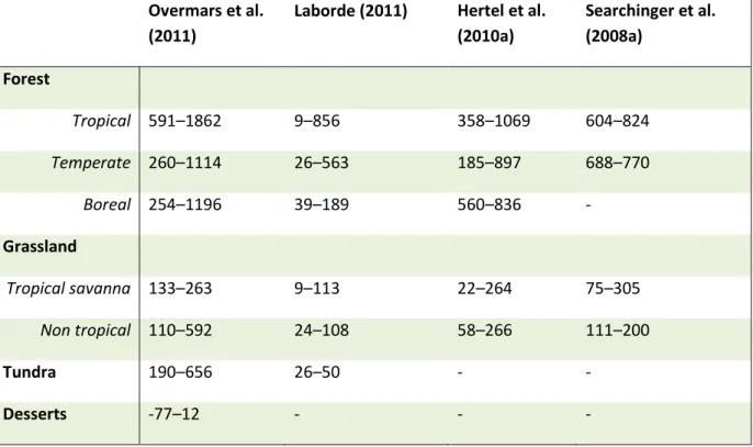
Land-cover change, finally, determines the level of conversion emissions. However, even emissions from a typical combination of land cover and region are uncertain. Overmars et al. (2011) reports a full range of emission factors, based on the literature (IPCC, 2001; Sabine et al., 2004): from an uptake of 77 tonnes CO2/ha as a minimum for the conversion of desert to cropland, to an emission of
1862 tonnes CO2/ha, the maximum for the conversion of tropical forest to cropland. In most
economic models, land-use emissions are not explicitly taken into account. The studies that report on those emissions use a combination of economic and biophysical models or derive the emissions from the calculated agricultural land use. The assumptions made in the previous steps are crucial for the final outcome. In addition, the assumed uptake in the reference scenario is important, with respect to the question of whether regrowth occurs on abandoned land. Another important issue is whether
2 The IMAGE model (Stehfest et al., 2014) allocates agricultural production per region to the existing
15
the wood residue from deforestation will be burned on location or removed and used as a product. Moreover, the amount of soil emissions assumed to be released over a particular time period differs between studies. Searchinger et al. (2008a), for example, attributed 25% of the soil carbon to the impact of biofuels. Finally, using an average emission factor per region resulted in different ILUC factors than from modelling the carbon cycle in a spatially explicit way, with emissions being calculated per location.
Table 1. Ranges of emission factors for the conversion of specific ecosystems to cropland, as used in ILUC literature (tonnes CO2/ha).
Overmars et al. (2011)
Laborde (2011) Hertel et al. (2010a) Searchinger et al. (2008a) Forest Tropical 591–1862 9–856 358–1069 604–824 Temperate 260–1114 26–563 185–897 688–770 Boreal 254–1196 39–189 560–836 - Grassland Tropical savanna 133–263 9–113 22–264 75–305 Non tropical 110–592 24–108 58–266 111–200 Tundra 190–656 26–50 - - Desserts -77–12 - - -
Conclusions
To determine ILUC, many assumptions have to be made, starting from the definition of sustainable biofuels to the value of very specific parameters for economic modelling or other calculation methods. Those different assumptions give a variety of results.
CGE models, which are frequently used in ILUC analyses, have been developed to analyse global trade patterns. They seem to be an appropriate choice of model – or the best we have available – in the sense of developments that could occur in production, consumption and trade, in general. However, one of the most important production factors for the agricultural sector is that of land. The costs involved and the corresponding dynamics, more specifically the physical limitations and
feedbacks to the production structures, are barely supported by scientific evidence. Incorporation of land in CGEs is still in its infancy (Schmitz et al., 2014). The agro-economic model comparison
conducted by Schmitz et al. (2014) shows that the strongest differences in model outcomes are related to the costs of land expansion, endogenous productivity responses, and assumptions about potential cropland. However, those processes are key with respect to ILUC emissions. The relatively small additional demand for land and biofuel needed under biofuel policy compared to the additional global demand for agricultural products and land, increase uncertainties even further. Although the
16
model seems to work quite well for historical analyses, the exact allocation of the ILUC effects and the related emissions largely influence the ultimate amount of ILUC emissions. Therefore, more accuracy would be required.
All together, this leads to the conclusion that, although these models may be the best we have, they do not seem to be appropriate for calculating ILUC emission factors. This argument counts even more when the results are used for policies that require exact point estimates per energy unit, such as the ILUC factors proposed in the EU Renewable Energy Directive (Plevin et al., 2010). Given the nature of the uncertainties, it seems they will not be narrowed down, in the near future. Therefore, monitoring and fundamental research has to be done. Comparing outcomes of different models may lead to a better understanding of the differences and identify blind spots. Using several model outcomes as a mean will not help to decrease the uncertainty, since the likelihood of results being accurate could differ between models.
Since no evidence exists that ILUC emissions would automatically stay within an acceptable range, policies are needed to prevent biofuels from becoming a source of climate change, instead of being part of the solution. Policymakers have to deal with the uncertainties and the adaptive possibilities of the economy; for example, as in the step from gross area to net area, shown in Figure 2. The
following section describes another approach of presenting ILUC, which provides insight into the adaptive efforts needed in the economy, while clearly identifying the uncertainties.
17
3. Reducing emissions from indirect land-use change to acceptable
levels
What would achieving an acceptable ILUC emission level require?
The Renewable Energy Directive has committed the European Commission to implement measures to avoid unacceptable ILUC emissions. The current method to manage ILUC is based on deriving ILUC factors from economic analyses (Laborde, 2011). However, as shown in the previous chapter, such an analysis introduces many uncertainties, especially in determining the net area, compared to the gross area needed to produce one Megajoule, due to lack of data and understanding.
This chapter approaches the ILUC problem the other way round; starting from an acceptable level of ILUC emissions and then work out what would be needed to achieve that level? Of course, the same parameters as discussed in Chapter 2 play their role. However, this approach gives insight into the efforts needed, for example, regarding yield increase or consumption change, in order to achieve this acceptable level of ILUC emissions. This approach also may be helpful in the consideration of
alternative or future policies.
The first step is to determine the maximum acceptable ILUC emission level (AIEL). Determining such a level would be a political choice. The presented calculation uses a maximum level of 21 gr CO2/MJ, as
an example. This level has been derived from the following argumentation: To ensure that the use of biofuels will decrease the emissions from fossil fuel use, a target for emission reductions in the biofuel chain has been set in the Renewable Energy Directive (RED) and the Fuel Quality Directive (FQD). Currently, the emission reduction in the production chain should be at least 35%, compared to the fossil fuel reference (84 gr CO2/MJ). In the near future, a minimum reduction of 60% for new
production facilities is required, in which no ILUC emissions are included. For our calculations, we simply maintained the minimum reduction of 35%, but now also including ILUC emissions. This implies an ILUC emission level of 25% (i.e. 60%-35%) of 84 gr CO2/MJ, or 21 gr CO2/MJ. These figures
only serve as an example.
Furthermore, we also has to include the amount of biofuels required to meet the biofuel blending mandate, as set in the RED and FQD. The higher the required amount of biofuels, the greater the required effort to avoid unacceptable ILUC emissions. Here, we assumed an additional biofuel production of 15.5 Mtoe (651 PJ), of which 72% in biodiesel (469 PJ) and the rest in bioethanol (182 PJ), based on the ratio between diesel- and petrol-fuelled vehicles. This results in a biofuel use of 8.6% in the total fuel use in 2020 (Laborde, 2011).
Given our AIEL and the assumed amount in order to comply with the RED and FQD, we analysed two cases. In both cases, land expansion for biofuel production is allowed up to 21 gr CO2/MJ in ILUC
emissions. For the first case, we analysed the yield increase from the current production area required to produce the rest of the biofuel production of 15.5 Mtoe. For the second case, we analysed the reduction in the consumption of non-biofuel products required to help realise the 15.5 Mtoe. These calculations illustrate the order of magnitude of the effort required and provide an indication of the risk that these aims will not be reached or may heavily impact other uses (in food and feed consumption and certain industry).
18
Energy yields from crops and related emissions from land-use conversion
First, the ILUC emission per MJ are presented, given a certain yield level and different levels of conversion emissions due to land-use change (Table 2). Per crop type, yields are shown for one main region, both including and excluding by-products. Of the by-products, 100% is assumed to be used for non-biofuel purposes. In addition to including the by-products, all other dynamics in Step 2 (Figure 2) are assumed not to change the land area needed. Since, after land-use conversion, biofuel crops may be grown on that land for many years to come, the conversion emissions have to be distributed over the total production period. Conversion emissions, thus, were evenly distributed over a period of 20 years, which is in line with the Renewable Energy Directive. This results in the following equation:
ILUC = (conversion emissions/20) / energy yield from one type of crop
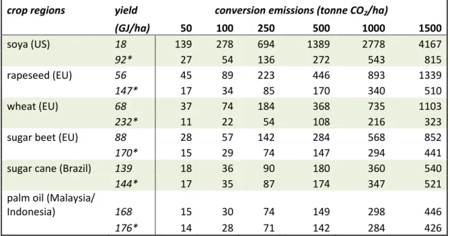
Table 2. ILUC emissions (gr CO2/MJ) at complete displacement for cases without counting for
byproducts, and including counting for byproducts
crop regions yield conversion emissions (tonne CO2/ha)
(GJ/ha) 50 100 250 500 1000 1500 soya (US) 18 139 278 694 1389 2778 4167 92* 27 54 136 272 543 815 rapeseed (EU) 56 45 89 223 446 893 1339 147* 17 34 85 170 340 510 wheat (EU) 68 37 74 184 368 735 1103 232* 11 22 54 108 216 323
sugar beet (EU) 88 28 57 142 284 568 852
170* 15 29 74 147 294 441
sugar cane (Brazil) 139 18 36 90 180 360 540
144* 17 35 87 174 347 521
palm oil (Malaysia/
Indonesia) 168 15 30 74 149 298 446
176* 14 28 71 142 284 426
Crops have been ranked from low to high yields, excluding by-products. For each crop type, the main production region is shown. Yields marked with * include the use of all by-products (Overmars et al., 2011).
Table 2 shows that the use of by-products could have an important impact, and that any type of land conversion with a conversion factor of 50 tonnes CO2/ha or less would stay below the acceptable
amount of ILUC emissions. Estimations of the emissions from conversions to cropland range between 110 and 592 tonnes CO2/ha for grasland, between 254 and 1196 tonnes CO2/ha for temperate and
boreal forests, and between 591 and 1862 tonnes CO2/ha for for tropical forests (Table 1). None of
the presented crops yield enough to stay below our AIEL at conversion levels of 100 tonnes CO2/ha
and more, even when accounting for complete use of the by-product. This means that emissions could only remain below our AIEL, if the net area needed is smaller than the gross area.
The conversion emissions shown in Table 2 have to be reduced to 21 gr CO2/MJ to stay below our
AIEL. This means that the gross area used, for example, for soya (first row, first column), with an ILUC emission factor of 139 gr CO2/MJ, has to be reduced by 85%. Conversions causing 100 tonnes CO2/ha
19
require an 80% reduction in gross area for crops yielding 50 GJ/ha. Conversions resulting in emissions of 250 tonnes CO2/ha require a reduction in gross area of 60% to 90%, for the crops presented in
Table 2. This reduction in land area should be achieved either through yield increases – in which case the biofuel mandate is assumed to trigger higher yields per hectare – or by consumption diversion. Consumption diversion means that, if the required reduction in net area is 60%, only 40% of the required mandate will be produced in addition to the current production level. The other 60% should come from current consumption. The following sections illustrate what this would mean, compared to the current situation.
Reducing net land use by increasing crop yields
Here, we describe the level of effort that would be needed to achieve the reductions in net area by increasing certain crop yields, assuming the complete use of by-products. This yield increase, in fact, should be in addition to the – assumed or expected – trend in normal yield increases. Because only in that case, ILUC emissions would really be avoided. To calculate the required effort, it is important to know the required biofuel production and the current production level (and land area) of a particular crop. Increasing the production by 1% on the currently used area, simply requires a yield increase of 1%. As explained above, we assume a production of 469 PJ for a biodiesel crop, or 182 PJ for a bio-ethanol crop. Thus, to realise the full mandate, at least two types of crops are needed. One should keep in mind that this ‘additional' yield increase should keep pace with the required additional biofuel production, in order to really avoid ILUC.
The results are presented in Table 3 in three different ways:
1) on regional crop area: yield increases are assumed to only take place in the region where the biofuel crop is being cultivated; for example, for biofuel produced from rapeseed in the EU, the yield increase should take place within the total EU rapeseed area (including other applications of the rapeseed).
2) on global crop area: the yield increases are assumed to take place at the global area of the specific crop type (again: no matter if crops are grown for biofuel or other purposes).
3) on total global crop area: an average yield increase per hectare of the total global cropland area; the biofuels are produced either from wheat and palm oil (minimum land-area case) or from sugar cane and soya (maximum land-area case). For this case, an additional production of 469 PJ biodiesel and 182 PJ bio-ethanol is assumed.
20
Table 3. Required yield increase to limit ILUC emissions to 21 gr CO2/MJ
conversion emissions (tonnes CO2/ha)
50 100 250 500 1000 1500
On regional crop area
soya (US) 3.8% 10.2% 14.1% 15.4% 16.0% 16.2%
rapeseed (EU)1 - 18.6% 36.7% 42.7% 45.7% 46.7%
wheat (EU) - 0.1% 1.8% 2.4% 2.7% 2.8%
sugar beet (EU) - 19.0% 47.4% 56.9% 61.6% 63.2%
sugar cane (Brazil) - 5.5% 10.6% 12.3% 13.2% 13.5%
palm oil (Malaysia/Indonesia) - 7.0% 19.0% 23.0% 25.0% 25.7% On global crop area
soya 1.1% 3.1% 4.2% 4.6% 4.8% 4.9% rapeseed - 3.7% 7.4% 8.6% 9.2% 9.4% wheat - 0.01% 0.2% 0.3% 0.3% 0.3% sugar beet - 6.6% 16.5% 19.8% 21.5% 22.0% sugar cane - 2.0% 3.9% 4.5% 4.8% 4.9% palm oil - 4.3% 11.7% 14.2% 15.4% 15.8%
On total global crop area
minimum: wheat and palm oil1 - 0.0% 0.2% 0.2% 0.2% 0.2%
maximum: sugar cane and soya1 0.0% 0.3% 0.4% 0.4% 0.4% 0.4%
100% use of by-products has been assumed, which is the most optimistic case. No consumption diversion takes place. ‘-‘ indicates no additional yield increase is necessary. 1In this case 469 PJ
biodiesel and 182 PJ bio-ethanol will be produced.
Table 3 shows that the required yield increases vary from 0% to 46.7%. If a specific crop is currently produced on a large area, the required average yield increase is relatively low (e.g. wheat). In that case, the production of biofuel can be spread over a larger area. Similarly, on the global level, the required yield increase is lower than on a regional level, because larger areas are involved. Although the yield increase per hectare is lower when more land area is involved, the total production effort is the same, as yields must be increased on all fields. This increase was assumed to take place within 10 years – as it should keep pace with the additional biofuel production – we simply divided this figure by 10, for an impression of the order of magnitude of the required annual increase. Historically, the average yield increase has been around 1% per year, for many crops. So one could argue that 10% (in Table 3) is considerable; doubling the yield increase with respect to the expected normal trend, or even 5% seems optimistic, given the debate about decreasing yield trends ((Alexandratos and Bruinsma, 2012; PBL, 2012). It should be noted that intensification (increasing yields per hectare) can also take place in the form of double cropping or using fallow land.
Taking a closer look at Table 3 shows that the figures for wheat, wheat and palm oil, and sugar cane and soya do not seem to be unrealistic, at least on a global level. The required effort in yield
development will be proportionally lower for each particular crop, if the bio-ethanol or biodiesel production is provided from more than one source. The two cases on the global level show the minimum effort needed to comply with the EU biofuel mandate. An annual increase in global
agricultural productivity of about 1% per year, with an additional 0.02% to 0.04% for only a relatively limited amount of biofuels in the EU shows the enormous challenge to sustainably produce much
21
larger amounts of biofuels for the global market. Since the target is set for 2020, the time in which to realise the calculated yield increase is only limited. Finally, it should be noted that only total yield increases can be monitored; additional yield increases due to a biofuel mandate can only be calculated.
Reducing net land use by reducing consumption
Another way to reduce the net area used for biofuel production is to also divert other forms of consumption at the same time. The impact of biofuel policies depends on the reduction in current consumption3 that is needed to ensure availability of the absolute amounts required for bio-ethanol
and biodiesel production. Similar to the previous section, we calculated the reduction in global consumption that would be required to achieve our AIEL (21 gr CO2/MJ). Again, we assumed that this
reduction would be sufficient to provide the required amounts of bio-ethanol (182 PJ) and biodiesel (469 PJ), depending on the particular crop. Table 4 shows the required reduction in consumption of the part of the crop that can be used for biodiesel or bio-ethanol. The consumption of by-products, such as meal or cake, does not have to be reduced.
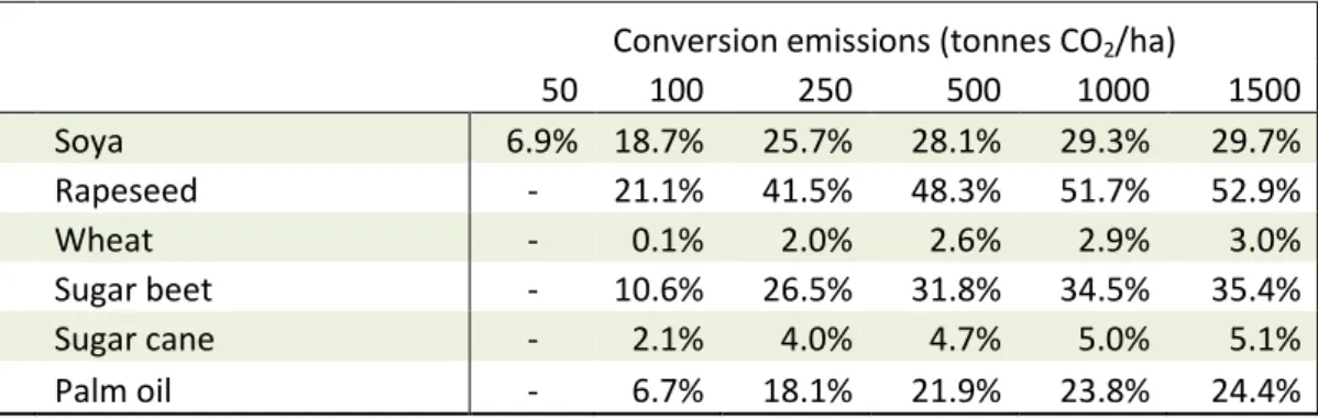
Table 4. Required reduction in consumption to limit ILUC emissions to 21gr CO2/MJ
Conversion emissions (tonnes CO2/ha)
50 100 250 500 1000 1500 Soya 6.9% 18.7% 25.7% 28.1% 29.3% 29.7% Rapeseed - 21.1% 41.5% 48.3% 51.7% 52.9% Wheat - 0.1% 2.0% 2.6% 2.9% 3.0% Sugar beet - 10.6% 26.5% 31.8% 34.5% 35.4% Sugar cane - 2.1% 4.0% 4.7% 5.0% 5.1% Palm oil - 6.7% 18.1% 21.9% 23.8% 24.4%
Table 4 shows that the required reduction in crop consumption for non-biofuel purposes is
considerable, also in the lower range of conversion emissions and especially for the biodiesel crops. The last could be expected, since around 70% of cars use diesel, and so 70% of the renewable target is expected to come from biodiesel crops. The required effort for diversion– as well as the required yield increase – will be proportionally lower if the bio-ethanol or biodiesel production will be provided from more than one source or if the target in the mandate would be lowered.
Of course, both yield increase and diversion could lead to the reduction in gross area that is required to stay below 21 gr CO2/MJ. This combination could range from a 100% yield increase and 0%
consumption diversion, to 0% yield increase and 100% consumption diversion.
What can we learn from these figures?
As shown in Chapter 2, a large part of the uncertainty in the current ILUC assessments concerns the step from gross to net area needed. Here, we make those uncertainties explicit by assuming an acceptable ILUC emission level and showing the efforts that are required to achieve that level. These efforts can be directed to improving agricultural productivity and/or changes in consumption
3 We assumed global production to be equal to global consumption; therefore, Table 4 is based on global
22
patterns. The results of our calculations show that, even for a limited amount in additional biofuels and a relatively high acceptable ILUC emission level, creating the conditions to produce these biofuels in a sustainable manner is not an easy task. The assumed amount of biofuel is crucial; requiring less bio-ethanol or biodiesel lowers the required efforts, linearly. Therefore, a decrease in the biofuel-blending target would limit the risk of producing higher ILUC emissions than would be.
23
4. Conclusions
The characteristics of indirect land-use change imply that impacts can hardly be monitored. Available model calculations give a range of values, while the implicit assumptions are usually not clarified. Furthermore, the uncertainties in parameters that define an important step within ILUC modelling are large. It is questionable if those uncertainties will be narrowed in the near future, due to lack of data and understanding.
Therefore, we followed another approach, to show the efforts that would be needed to keep ILUC emissions below a certain level for a range of final conversion emissions. We have chosen an acceptable ILUC emission level of 21 gr CO2/MJ.
The calculation shows that if the direct land use (gross area) would be the same as the indirect land use (net area), this ILUC level would be exceeded for a large range of land-conversion emissions. Even land conversion that cause emissions of approximately 100 tonnes CO2 per hectare – which
corresponds with conversions from grassland to cropland – would not be acceptable. Yield increases or diverged consumption are needed to keep ILUC emissions below 21 gr CO2/MJ.
The required effort in yield increase, for a given crop, varies under different assumptions. The larger the current cropland area within the agricultural system, the smaller the required yield increase per hectare. This means that the effort needed to achieve yield increases is low for wheat and high for palm oil. The last requires about 12% to 20% increase in yields for land conversions causing emissions in the range of 250 to 1000 tonnes CO2 per hectare. Increasing yields over the total agricultural area
results in a minimal effort per hectare, but requires an extensive effort from the perspective of the total land area involved.
The impact of consumption diversion is indicated here by the required reduction in total
consumption in order to stay below the acceptable ILUC emission level. Again, the current level of consumption determines the impact of the required diversion. Required diversion in the wheat sector is small, and therefore seems to be without large impacts on other consumption purposes. The required diversion in the rapeseed sector, in contrast, requires up to 53% reduction in the current consumption.
The amount of effort that is required is indicative of the conditions that should be created, in order to produce the biofuels sustainably. The figures indicate that achieving a certain level of ILUC emissions is not without costs, even at low conversion emission levels. Moreover, the target of the EU biofuel mandate is set for 2020, and therefore the time period for creating these conditions is limited. Limiting the required mandate to an amount that results in reasonable efforts in required yield increase or consumption diversion would reduce the risk of ILUC emissions exceeding the acceptable level. The proposal of the European Commission to place a 5% cap on the use of food crops fits into that conclusion.
24
References
Alexandratos, N. and J. Bruinsma (2012). World agriculture towards 2030/2050: the 2012 revision. ESA Working paper. Rome, FAO. 12-03.
Edwards, R., D. Mulligan and L. Marelli (2010). Indirect land use change from increased biofuels demand. Comparison of models and results for marginal biofuels production from different feedstocks. Luxemburg, JRC Institute for Energy.
Eickhout, B., H. Van Meijl, A. Tabeau and E. Stehfest (2009). The impact of environmental and climate constraints on global food supply. Economic analysis of land use in global climate change policy. T. Hertel, S. K. Rose and R. Tol. London, Routledge.
EU (2009a). Directive 2009/28/EC. Official Journal of the European Union L 140, 16-62. EU (2009b). Directive 2009/30/EC. Official Journal of the European UnionL140, 88-113.
FAO (2012). FAOSTAT database collections. Rome, Food and Agriculture Organization of the United Nations.
Gibbs, H. K., A. S. Ruesch, F. Achard, M. K. Clayton, P. Holmgren, N. Ramankutty and J. A. Foley (2010). "Tropical forests were the primary sources of new agricultural land in the 1980s and 1990s." Proceedings of the National Academy of Sciences of the United States of America 107(38): 16732-16737.
Golub, A. A. and T. W. Hertel (2011). Modelling land use change impacts of biofuels in the GTAP-BIO Framework. Paper prepared for special issue of Climate Change Economics, Purdue
University.
Hertel, T., D. Hummels, M. Ivanic and R. Keeney (2007). "How confident can we be of CGE-based assessments of Free Trade Agreements?" Economic Modelling 24(4): 611-635.
Hertel, T. W., A. A. Golub, A. D. Jones, M. O'Hare, R. J. Plevin and D. M. Kammen (2010a). "Supporting online material for: Effects of US Maize Ethanol on Global Land Use and Greenhouse Gas Emissions: Estimating Market-mediated Responses." Bioscience 60(3): 223-231.
Hertel, T. W., W. E. Tyner and D. K. Birur (2010b). "The global impacts of biofuel mandates." Energy Journal 31(1): 75-100.
IPCC (2001). Climate Change 2001: The Scientific Basis. Contribution of Working Group I to theThird Assessment Report of the Intergovernmental Panel on Climate Change. J. T. Houghton, Y. Ding, D. J. Griggset al. Cambridge/NewYork, Cambridge University Press: 881.
Kavallari, A., E. Smeets and A. Tabeau (2014). "Land use changes from EU biofuel use: a sensitivity analysis." Operational Research 14(2): 261-281.
Keeney, R. and T. W. Hertel (2008). The Indirect Land Use Impacts of U.S. Biofuel Policies: The Importance of Acreage, Yield, and Bilateral Trade Responses. Purdue.
Laborde, D. (2011). Assessing the land use change consequences of European Biofuel Policies, ATLASS Consortium.
Laborde, D. and H. Valin (2012). "Modeling land-use changes in a global CGE: Assessing the EU biofuel mandates with the Mirage-BioF model." Climate Change Economics 03(03): 1250017. Overmars, K. P., E. Stehfest, J. P. M. Ros and A. G. Prins (2011). "Indirect land use change emissions
related to EU biofuel consumption: an analysis based on historical data." Environmental Science & Policy 14(3): 248-257.
PBL (2012). Roads from Rio+20. Pathways to achieve global sustainability goals by 2050. the Hague, Netherlands Environmental Assessment Agency.
Plevin, R. J., M. O’Hare, A. D. Jones, M. S. Torn and H. K. Gibbs (2010). "Greenhouse Gas Emissions from Biofuels’ Indirect Land Use Change Are Uncertain but May Be Much Greater than Previously Estimated." Environmental Science & Technology 44(21): 8015-8021.
Prins, A. G., E. Stehfest, K. P. Overmars and J. P. M. Ros (2010). Are models suitable for determing ILUC factors. Bilthoven, Netherlands Environmental Assessment Agency.
Ros, J. P. M., K. P. Overmars, E. Stehfest, A. G. Prins, J. Notenboom and M. Oorschot (2010). Identifying the indirect effects of bio-energy production. Bilthoven, Netherlands Environmental Assessment Agency.
25
Sabine, C. L., M. Heimann, P. Artaxo, D. C. E. Bakker, C.-T. A. Chen, C. B. Field, N. Gruber, C. Le Quere, R. G. Prinn, J. E. Richey, P. Romero, J. A. Sathaye and R. Valentini (2004). Current status of past trends of the global carbon cycle. Global Carbon Cycle, Integrating Humans, Climate and the Natural World. C. Field and M. Raupach. Washington DC, Island Press: 17–44.
Salhofer, K. (2000). Elasticities of Substitution and Factor Supply Elasticities in European Agriculture: A Review of Past Studies. Diskussionspapier Institut für Wirtschaft, Politik und Recht
Universität für Bodenkultur Wien.
Schmitz, C., H. van Meijl, P. Kyle, G. C. Nelson, S. Fujimori, A. Gurgel, P. Havlik, E. Heyhoe, D. M. d'Croz, A. Popp, R. Sands, A. Tabeau, D. van der Mensbrugghe, M. von Lampe, M. Wise, E. Blanc, T. Hasegawa, A. Kavallari and H. Valin (2014). "Land-use change trajectories up to 2050: insights from a global agro-economic model comparison." Agricultural Economics 45(1): 69-84.
Searchinger, T., R. Heimlich, R. A. Houghton, F. Dong, A. Elobeid, J. Fabiosa, S. Tokgoz, D. Hayes and T.-H. Yu (2008a). "Supporting online material for: Use of U.S. Croplands for Biofuels Increases Greenhouse Gases Through Emissions from Land-Use Change." Science 319(5867): 1238-1240.
Searchinger, T., R. Heimlich, R. A. Houghton, F. Dong, A. Elobeid, J. Fabiosa, S. Tokgoz, D. Hayes and T.-H. Yu (2008b). "Use of U.S. Croplands for Biofuels Increases Greenhouse Gases Through Emissions from Land-Use Change." Science 319(5867): 1238-1240.
Spera, S. A., A. S. Cohn, L. K. VanWey, J. F. Mustard, B. F. Rudorff, J. Risso and M. Adami (2014). "Recent cropping frequency, expansion, and abandonment in Mato Grosso, Brazil had selective land characteristics." Environmental Research Letters 9(6): 064010.
Stehfest, E., D. P. Van Vuuren, T. Kram, L. Bouwman, R. Alkemade, M. Bakkenes, H. Biemands, A. Bouwman, M. Den Elzen, J. Janse, P. Lucas, J. G. Van Minnen, C. Müller and A. G. Prins (2014). Integrated Assessment of Global Environmental Change with IMAGE 3.0. The Hague, PBL Netherlands Environmental Assessment Agency.
Taheripour, F., T. W. Hertel, W. E. Tyner, J. F. Beckman and D. K. Birur (2010). "Biofuels and their by-products: Global economic and environmental implications." Biomass and Bioenergy 34(3): 278-289.
Van Asselen, S. and P. H. Verburg (2012). "A land system representation for global assessments and land-use modeling." Global Change Biology 18: 3125–3148.
Wicke, B., P. Verweij, H. van Meijl, D. P. van Vuuren and A. P. Faaij (2012). "Indirect land use change: review of existing models and strategies for mitigation." Biofuels 3(1): 87-100.