RIVM report 260706001/2005
A conceptual framework for budget allocation in the RIVM Chronic Disease Model.
A case study of Diabetes mellitus.
RT Hoogenveen, TL Feenstra, PHM van Baal, CA Baan
This investigation has been performed by order and for the account of the RIVM, within the framework of project S/260706, Priority setting in chronic diseases: methodology for budget allocation.
RIVM, P.O. Box 1, 3720 BA Bilthoven, telephone: 31 - 30 - 274 91 11; telefax: 31 - 30 - 274 29 71
Contact: TL Feenstra
Department for Prevention and Health Services Research (PZO) Talitha.Feenstra@rivm.nl
Rapport in het kort
Conceptueel model voor budgetallocatie met het RIVM Chronische Ziekten Model. Toepassing bij Diabetes mellitus.
Dit rapport beschrijft de elementen van een zogeheten ‘budget allocatie model’. Dit model is bedoeld ter ondersteuning van beleidsmakers bij keuzes over de inzet van budget voor primaire preventie en/of preventie in de zorg bij chronische
aandoeningen. Als concrete toepassing is gekozen voor Diabetes mellitus. Een uitbreiding van het RIVM Chronische Ziekten Model beschrijft het verband tussen diabetes, risicofactoren en hart- en vaatziektecomplicaties. Een
gezondheidseconomische module berekent vervolgens gezondheidseffecten in termen van gewonnen levensjaren en voor kwaliteit van leven gecorrigeerde gewonnen levensjaren (QALYs), interventiekosten, en kosten van zorg. Ten slotte bespreken we hoe de voorkeuren van beleidsmakers kunnen worden geformaliseerd in
doelstellingsfuncties en (budget-)beperkingen.
Deze drie elementen zijn de basis voor een toepassing van budgetallocatie bij diabetes. De ontwikkelde methode is ook toepasbaar bij andere chronische ziekten, omdat we het bredere RIVM Chronische Ziekten model als uitgangspunt hebben gebruikt. Het nieuwe model voor diabetes is niet alleen een basis voor
budgetallocatie, maar ook op zichzelf al bruikbaar om primaire preventie en verschillende vormen van preventie van complicaties bij diabetes te evalueren. Het model kan voor deze interventies de consequenties voor Nederland berekenen, zowel voor de kosten van zorg als voor de gezondheid.
Abstract
A conceptual framework for budget allocation in the RIVM Chronic Disease Model. A case study of Diabetes mellitus.
The research project ‘Priority setting in chronic diseases: methodology for budget allocation’ aims to develop a methodology to support optimal allocation of the health care budget with respect to chronic diseases.
The current report describes the modelling steps required to address budget allocation questions regarding the prevention of chronic diseases and their complications with the RIVM Chronic Disease Model, with specific attention to diabetes mellitus. An extension of the RIVM Chronic Disease Model deals with the links between diabetes, its risk factors and its macrovascular complications. A health economics module computes outcomes in terms of intervention costs, costs of care and composite health effects. Finally, it is discussed how to formalize different preferences of policy makers in various objective functions and constraints.
These three elements form the basis for the analysis of budget allocation questions in diabetes care. The model allows for the comparison of primary prevention with the prevention of complications in diagnosed patients as to costs of care and health effects. Furthermore, as it stands, the model with the health economics module per se is a useful tool for policy analysis, for instance, to compare the costs and effects of different interventions.
Voorwoord
Het MAP SOR-onderzoeksprogramma ‘Methodologie optimale gezondheidswinst en kwaliteit van zorg’ wijst op het strategisch belang van methodeontwikkeling ter ondersteuning van optimale inzet van het gezondheidszorgbudget. Het project ‘Budgetallocatie: methode-ontwikkeling voor prioritering van interventies bij chronische ziekten (Priority setting in chronic diseases: methodology for budget allocation)’ sluit daarbij aan, en beoogt bij te dragen aan de methodes voor het
vergelijken van de kosten en effecten voor preventieve screenings en zorginterventies. Daartoe zal een zogeheten budgetallocatiemodel worden ontwikkeld. Het
onderzoeksproject richt zich daarbij vooral op die budgetallocatieproblemen die net een stap verder gaan dan traditionele kosteneffectiviteitsanalyses en bijvoorbeeld afwegingen maken tussen verschillende types interventies voor een ziekte. Er wordt gestreefd naar methodologie die voor verschillende (chronische) aandoeningen toepasbaar is. Daarbij is voor diabetes gekozen als eerste voorbeeldstudie.
Het voorliggende rapport beschrijft de conceptuele en formele opzet van een diabetes model wat geschikt is als basis voor budgetallocatie (hoofstukken 2 en 3). Daarnaast wordt de benadering voor budgetallocatie conceptueel uitgewerkt (hoofdstuk 4). Het onderzoek voor de hoofdstukken over het diabetesmodel in dit rapport is
uitgevoerd in nauwe samenwerking met de onderzoekers die waren betrokken bij de beantwoording van de kennisvraag ‘Preventie van diabetes’. Het werk aan en de rapportage voor beide projecten is op elkaar afgestemd, om dubbelingen te
voorkomen. Daarbij zullen de inhoudelijke onderdelen worden gerapporteerd in het rapport ‘Modelling Chronic Diseases: the diabetes module. Justification of (new) input data in the mathematical RIVM Model’, terwijl in dit rapport de conceptuele en formele opzet van het model is beschreven. Dit onderzoeksproject bouwt gedeeltelijk voort op eerder werk over het onderwerp budgetallocatie in het kader van het
ZONMW programma doelmatigheid. De gezondheidseconomische module die een van de bouwstenen vormt van het budgetallocatiemodel is beschreven in het rapport ‘Cost Effectiveness Analysis with the RIVM Chronic Disease Model’. Tenslotte willen we Hendriek Boshuizen en Guus Den Hollander bedanken voor nuttig commentaar bij conceptversies van het rapport.
Contents
Summary 6
1. Introduction 7
1.1 Background 7
1.2 Cost effectiveness analysis and budget allocation 7
1.3 Scope of the budget allocation model 8
1.4 A case study of diabetes mellitus 9
1.5 Overall aim of the project and content of the current report 10 2. A model for evaluation of interventions for the case of diabetes 11
2.1 Review of existing models in the literature 11
2.2 Model structure 12
2.2.1 The RIVM chronic disease model 12
2.2.2 A diabetes model suitable for budget allocation 13 3. A model of diabetes and macrovasculair complications in relation to risk factors. 17 3.1 The RIVM Chronic Disease model, CDM2005 joint version 17 3.2 The new model of diabetes and macrovasculair complications in relation to risk factors: input data 21
3.2.1 Population numbers 21
3.2.2 Prevalence of DM and riskfactors in startyear 21
3.2.3 Transitions in a year 22
3.2.4 Relative risks 23
3.2.5 Costs of care for each disease stage 23
3.2.6 Quality of life in each disease stage 24
3.3 Methodological issues in a diabetes model, formal solutions in CDM2005 joint version 24
3.3.1 Model initialization steps 25
3.3.2 Model simulation steps 35
3.3.3 Effects of treatment. 38
4. Budget allocation in a Chronic Disease Model: methodological issues 39
4.1 Background and state of the art 39
4.2 Formalization of the budget allocation problem 42
4.3 Budget allocation in the RIVM CDM. 45
4.4 Methodological issues 50
4.5 Example interventions 51
5. Discussion and Conclusions 53
References 55
Appendix 1 Models on complications of diabetes mellitus 61
Appendix 2 Adjustment factors for intermediate diseases 64
Summary
IntroductionThe research project ‘Priority setting in chronic diseases: methodology for budget allocation’ is aimed at developing a methodology to support optimal allocation of the health care budget with respect to chronic diseases. Diabetes is an interesting
example, because many different options for primary prevention and the prevention of complications exist.
Objective
The aim of the current report was to describe the modelling steps required to address budget allocation questions for the prevention of chronic diseases, with specific attention for diabetes.
Methods
The scope of the budget allocation problem was limited to either the case of a single disease, or the case of a single type of interventions. Based on the RIVM chronic disease model, a multistate transition model was developed with joint states
representing individuals’ risk factor and disease status. Specific attention was paid to the modelling of diabetes, our example for the single disease case. A health
economics module enabled the computation of total costs, intervention costs, total effects and cost-effectiveness ratios. Finally, the conceptual approach to budget allocation was developed, using mathematical programming to formalize the problem, and paying attention to objective functions and budget constraints.
Results
The result of the modelling efforts is a set of formal equations defining the elements relevant for diabetes in the RIVM Chronic Disease Model 2005 joint version and a health economics module. The implementation of these in mathematica has to be combined with estimates of the input data. Then, the model is ready for the evaluation of different prevention interventions for diabetes and its macrovascular complications. Budget allocation problems can then be addressed by adding an objective function and formulating the relevant constraints. The resulting optimisation problem may be solved either in a single step or in a two step procedure, first generating results from scenario analysis of the model and then optimizing over these outcomes.
Conclusion
The implemented model will enable us to evaluate both interventions for the primary prevention of diabetes and interventions in diabetes patients to prevent macrovascular complications. This forms the basis for the analysis of budget allocation questions in diabetes care. The general structure of our budget allocation model is not limited to diabetes and is intended to be applicable for any chronic disease. The disease model per se is a useful tool to give policy relevant information in combination with the health economics module, for instance, the costs and effects of different interventions can be compared.
1.
Introduction
1.1
Background
The research project ‘Priority setting in chronic diseases: methodology for budget allocation’ is aimed at developing a methodology to support optimal allocation of the health care budget with respect to chronic diseases. A so-called budget allocation model will be set up, this is an explicit model of the objectives and constraints faced by decision makers in their choices between different health care interventions. The explicit formulation of the model helps to analyse several issues that complicate matters for the decision maker. Thus, we hope to make the issue of budget allocation more transparent and insightful for decision makers. In this introductory chapter the economic and epidemiological background for this project are described. First, the problem of budget allocation and its relation with cost effectiveness analysis is explained. Second, the scope of the budget allocation model for this project is
described. The next section introduces diabetes mellitus, which was the case study for this project. The chapter ends with a description of the report’s aim and contents.
1.2
Cost effectiveness analysis and budget allocation
Economic evaluation has been developed as a tool to inform policy makers about the costs and effects of medical interventions to support their decisions on the optimal allocation of health care resources. Usually cost effectiveness analyses compare the outcomes of two or more alternatives and result in a cost-effectiveness ratio, which expresses how much money has to be paid per additional unit of health gained (for instance, life years (LY’s) or quality adjusted life years (QALY’s) gained). The lower this ratio, the more cost effective it is to implement the investigated intervention. That is, the more health effects are obtained for given expenditures. Some interventions turn out to be dominant, because they are less costly and, at the same time, generate more health effects than their comparator. Other interventions result in better health but at additional costs.
To support decision makers in allocating money to different interventions in health care, a cost effectiveness ratio alone, though useful, may not be sufficient. In addition, decision makers may also need information that more explicitly addresses the issue of budget allocation and for instance compares the total costs and effects of interventions (so called budget impact analyses), or even explicitly formulates the objectives and constraints in a budget allocation model. To estimate the total effects and costs of interventions over time often more epidemiological data and demographic data is needed than in ordinary cost effectiveness analyses. For instance, the number of patients requiring certain treatments is needed to compute the total costs of the intervention, while a cost effectiveness analysis can be based on the costs per patient. Consider a decision maker that wants to allocate his budget over different treatments for the same chronic disease. Assume that he has the choice between supporting a (tertiary) prevention program targeted at a large group of patients in mild stages of the disease, with a cost effectiveness ratio of 31000 per LY gained or supporting a new
surgical procedure with exactly the same cost effectiveness ratio, but targeted at patients in the more advanced stages of the disease. That is, the net present values of the incremental costs and effects of both interventions are equal. Of course, they differ widely in the distribution of these costs and effects over time. They may also differ in their budgetary consequences. Assuming that the total health effects and costs of different interventions are available, the next question is how the decision maker should go on to compare the efficiency of these interventions? If the prevention program effectively limits the number of patients in need of surgical procedure, then it is clear that the total costs and effects of the interventions considered are
interdependent. Such interdependencies require a model where time enters explicitly. Budget allocation models combine the results of cost effectiveness analysis with epidemiological and demographic data, an optimality criterion, and budget constraints to find the optimal allocation of resources over programs. The best-known budget allocation model has maximization of the sum of health effects as its optimality criterion, under the constraint that the sum of program costs remains within a given total budget.1 We refer to this model as the standard model. The current report describes the modelling steps required to address budget allocation questions for the prevention of chronic diseases and their complications, with specific attention for diabetes mellitus.
1.3
Scope of the budget allocation model
It is our aim to develop a methodology to support optimal allocation of the health care budget with respect to chronic diseases that enables one to compare the costs and health effects of primary prevention with secondary prevention (screening) and tertiary prevention (prevention of complications in diagnosed patients). To enable this, the first step in the development of the budget allocation model is to ensure that different interventions can be compared in terms of costs and effects. The comparison of health costs and effects and cost effectiveness ratio’s from different studies is surrounded by difficulties because of differences in adopted methodologies, perspective and differences in data sources.
To develop a method to consistently deal with health effects and costs on the population level we used the RIVM Chronic Disease Model (CDM) 2. This is a multistate transition model that links prevalence of risk factors to the incidence of 28 chronic diseases. The model allows to compute the effects of a reduction in risk factors through prevention on life years gained and quality of life, taking account of comorbidity. The CDM models the entire Dutch population, following the life course of birth cohorts over time and thus allows to estimate the total costs and health effects of interventions for the entire Dutch population. By using the CDM to compute health effects and costs it can be ensured that the same methodology and the same type of costs and effects are taken into account for all different interventions that are compared 3. The RIVM Chronic Disease Model was intended primarily as tool to model the health effects of primary prevention. Since our aim is to also compare primary with secondary and tertiary prevention and to use economic as well as health outcomes, the CDM must be adjusted in several ways. As a guide for these
adjustments in the CDM and in the development of the budget allocation model diabetes was chosen as a case study.
1.4
A case study of diabetes mellitus
Diabetes mellitus is a major source of morbidity and mortality, associated with serious complications, loss in quality of life and high use of health care.4 5 In the recent
decades, the incidence and prevalence of diabetes have increased and it was estimated that the number of diabetic patients in the Netherlands will increase with 36% in 2020 due to demographic trends only. 6 7 It is to be expected that this increase will be even larger, considering the observed trends in obesity and physical inactivity.8 The present health care system is not optimally organized for an adequate treatment and control of chronic diseases like type 2 diabetes, the health care budget for prevention is limited, and the burden for health care providers is high. Therefore, it is of great importance to know which type of prevention strategy for diabetes provides the largest gain in terms of health (quality of life, life years gained) and in terms of savings in health care use relative to its input requirements.
The severity and prevalence of the disease make diabetes a candidate for various prevention strategies. However, to be able to quantify more accurately the choice of strategy, requires knowledge on the (side-)effects of the possible strategies. Three types of prevention strategies of diabetes exist: primary, secondary and tertiary prevention. The aim of primary prevention is to prevent the development of diabetes in high risk individuals in the general population. Several risk factors of diabetes have been identified, with overweight and lack of physical activity being the major ones. The aim of secondary prevention is the early detection and subsequently treatment of patients with yet undiagnosed diabetes. About half of patients with diabetes is yet undiagnosed.6 Tertiary prevention aims at obtaining health gains by the delay or even prevention of complications as a result of intensive follow-up and treatment of diagnosed diabetes patients. Several clinical trials demonstrated that a good glycemic control as well as adequate control of lower leg morphology, and treatment of risk factors for cardiovascular diseases (hypertension, dyslipidemia, overweight, smoking) can considerably limit the incidence of diabetes complications.9 10
To obtain reliable estimates for the Dutch situation, it is necessary to analyze and compare different interventions in the same setting, using one model and comparable epidemiological outcome and cost data for all interventions. For primary prevention of diabetes this has been done by the iMTA in collaboration with the WHO.11 12 Many economic evaluations of single or combined strategies for the prevention of
macrovascular complications exist. 13 14 Earnshaw15 evaluated different combinations of four interventions, all aiming at the prevention of complications in diabetes patients and used budget allocation methods to find optimal allocations for different objectives and constraints. He used the CDC diabetes model, representing the USA situation as a basis. In our case study, we want to compare both interventions for primary
1.5
Overall aim of the project and content of the
current report
In short, this research project should result in budget allocation models that inform decision makers on the optimal allocation for different objectives or constraints. The strict assumptions of the standard model involve a fixed patient group, a single budget constraint, and a static model without attention for the distribution of costs and effects over time. This standard model underlies the decision rules of cost effectiveness analyis. By choosing diabetes as a case study, we hope to tackle a lot of the methodological issues that can be encountered if one wants to compare primary prevention with secondary and tertiary prevention. The general structure of our budget allocation model is not limited to diabetes and is intended to be applicable for any chronic disease. In a second case, different interventions in primary prevention (smoking cessation and interventions to reduce overweight) will be compared. To set up the budget allocation model for the diabetes case study, the following research questions have to be answered :
• What are the characteristics of a diabetes model that can be applied for budget allocation?
• What data are available to populate a model presenting the Dutch situation? • What additional modeling is needed to actually perform a budget allocation
analysis?
• What methodological issues arise and which are relevant to approach? To answer these questions, the following topics will be addressed in the current report. To characterize a diabetes model suitable for budget allocation, first, a review is given of existing diabetes models (section 2). Second, the structure of a diabetes model that is suitable for budget allocation is described (section 2), starting with a description of the current diabetes model in the RIVM Chronic Disease Model. Third, the formal approach to the diabetes model is outlined (section 3) and the data
requirements to estimate model parameters are described (section 3). The estimates of these parameters will be reported in this report’s twin report for the diabetes model.16. Fourth, section 4 shortly describes the health economics module,16 contains a
description of the aims of budget allocation, and introduces the additional
requirements to perform a budget allocation analysis based on this model together with the methodological issues to be addressed. Finally section 5 concludes with a summary and discussion of the results.
2.
A model for evaluation of interventions for the
case of diabetes
The model was based on the existing diabetes module in the RIVM Chronic Disease Model.2 However, this model had to be updated and extended to allow for explicit modelling of diabetes complications in relation to risk factors. This section starts with a description of diabetes models in the literature and what can be learned from then, followed by an explanation of the changes made on the Chronic Disease Model (CDM).
2.1
Review of existing models in the literature
The modelling work in the project was started with a scan of the literature on existing diabetes models, to put our work into perspective and to see whether any models suitable for budget allocation already existed. A summary of the review is given in appendix A.
From an examination of the characteristics of the models identified, three
observations may be made. First, the number of different models is quite limited, because many models were adjustments of others. For microvascular complications, one standard structure exists, for instance described in publications on the UKPDS model. 17 18 Mortality was only increased for the most severe microvascular
complication stages (blindness, ESRD, amputation). For macrovascular complications, most models were based on the Framingham risk functions,19 sometimes with added modelling to enable for recurrent events. Second, for
microvasculair complications, the most important explanatory variables used in the models were diabetes duration and HbA1c, while for macrovascular complications these were age, sex, SBP, cholesterol ratio, and smoking status. Third, most models described stochastic individual life courses using discrete time steps of 1 year. Few models were time continuous and deterministic, but these did not include duration as an explanatory variable.
Important sources for parameter estimates used in many models were the Diabetes Control and Complications Trial (DCCT) 20, the United Kingdom Prsopective Diabetes Study (UKPDS) 21, the Wisconsin Epidemiologic Study of Diabetic Retinopathy22, and the Framingham Heart Study.19 The risk functions of the latter were often used for the cardiovascular complications. Simulation models have been developed based on each large follow-up study, such as UKPDS and DCCT. To conclude, most models focussed on microvascular complications and modelled macrovascular complications in less detail. From a budget allocation point of view, the macrovascular complications deserve more attentions, since they account for about 40% of total costs of care related to diabetes, while microvascular
complications account for about 10%. 23 Two models with extensive modeling of macrovascular complications were the UKPDS-model 17 and the Swiss model by Palmer et al..24-26
2.2
Model structure
This subsection describes the general set up of a chronic disease model with diabetes suitable for budget allocation over all types of prevention.
2.2.1 The RIVM chronic disease model
The current model (CDM2003) has been described previously.2 27
In short, the RIVM Chronic Disease Model (CDM) has been developed as a tool to describe the morbidity and mortality effects of autonomous changes of and
interventions on chronic disease risk factors taking into account integrative aspects. The model contains the following risk factors: cholesterol, systolic blood pressure, smoking, physical activity level, and Body Mass Index. It models 28 chronic diseases: cardiovascular diseases, distinguishing acute myocardial infarction, other coronary heart disease, stroke, and chronic heart failure, COPD, asthma, diabetes mellitus, dementia, several musculoskeletal disorders, and 15 different forms of cancer.
The mathematical model structure is called a multi-state transition model and is based on the life table method. The model states defined are the risk factor classes and disease states. State transitions are possible due to changes between classes for any risk factor, incidence, remission and progress for any disease, and mortality. The model describes the life course of cohorts in terms of changes between risk factor classes and changes between disease states over the simulation time period. Risk factors and diseases are linked through relative risks on disease incidence. That is, incidence rates for each risk factor class are found as relative risks times baseline incidence.
The main model parameters are: • the initial population numbers
• initial class prevalence rates and transition rates for all risk factors
• initial prevalence, incidence, remission and mortality rates for all diseases and • relative risk values specified by risk factor and chronic disease
All model parameters and variables are specified by gender and age. The time step used for modeling is 1 year.
The main model outcome variables are incidence, prevalence and mortality numbers specified by disease, and integrative measures such as total and quality-adjusted life years.
The CDM2003 model describes risk factor class prevalence and disease prevalence numbers separately. For example, the model keeps track of the number of smokers and non-smokers, and the number of persons without and with diabetes, but not of the number of persons with diabetes who smoke. It takes account of the dependency relations between risk factors and diseases through a time-dependent covariance matrix. The CDM2005 joint version which will be presented below describes the joint prevalence numbers explicitly. For example, the number of non-smokers without diabetes, non-smokers with diabetes etcetera.
2.2.2 A diabetes model suitable for budget allocation
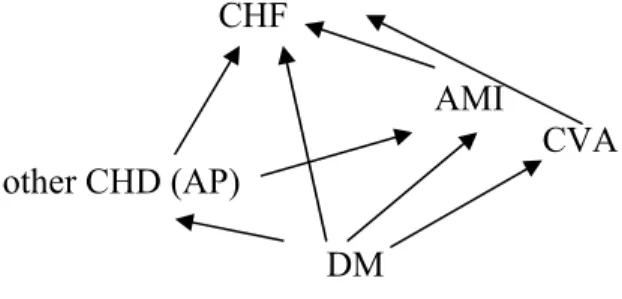
Diabetes is one of the 28 chronic diseases which is explicitly modeled in CDM. To allow for analysis of the complications of diabetes, diabetes is modeled both as a disease and a risk factor for some other diseases, that is, an intermediate disease. Some cardiovascular diseases are also intermediate diseases in CDM. Figure 1 shows the causal dependency structure between diabetes and cardiovascular diseases.
CHF
AMI
CVA other CHD (AP)
DM
Figure 1: Causal dependency relations between diabetes mellitus and several cardiovascular diseasesi
i
CHF=Chronic heart failure, AMI= Acute Myocardial infarction, other CHD=other Coronary diseases (AP=Angina pectoris), CVA=Stroke (cardiovascular accident), DM=Diabetes Mellitus
For each pair of diseases the incidence rate ratios of the ‘end’ disease are adjusted for incidence through the ‘intermediate’ disease (see section 3.3.1.2).
The following risk factors included in the current model are important for the modelling of diabetes and its complications:
• Body Mass Index (BMI) • physical activity
• smoking
• total cholesterol
• Systolic Bloodpressure (SBP)
For all risk factors, the model distinguishes several classes, for instance normal weight (BMI<25), overweight (BMI 25-30) and obese BMI (BMI >30).
In CDM2003, BMI and physical activity are risk factors for diabetes incidence as well as for some other cardiovascular diseases. Smoking, cholesterol and blood pressure are modeled as risk factors for cardiovascular diseases.
Adding these risk factors for diabetes (BMI and activity) and its complications to the figure above, a rather complex structure results.
Risk factors for diabetes incidence and cardiovascular diseases Risk factors for cardiovascular diseases
Cardiovascular diseases (macro vascular diabetes complications)
Figure 2: Structure of dependency relations between risk factors, diabetes mellitus and several cardiovascular diseases.
Simplifying this structure (see Figure 3), the CDM2003 marginal model catches the link between risk factors, diabetes and its complications, but does not keep track of the risk factors for people with diabetes.
Therefore, the model is fit to evaluate the effects of primary prevention, since the effect of changes in risk factor prevalences on diabetes and on complications can be analysed. However diabetes is modeled as a single stage disease and in the model the risk of complications is not different for a person with diabetes with or without e.g. high blood pressure. Therefore, the model is not fit to evaluate the effect of tertiary prevention, that is the prevention of diabetes complications resulting from improved care. Hence, an extension of the model is needed to allow for the evaluation of tertiary prevention.
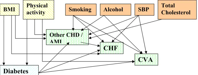
To be able to evaluate prevention of complications, the model was to be extended to include the prevalence of risk factors for macrovascular complications in diabetes, as follows (see Figure 4):
Figure 3: Simplified structure of dependency relations between risk factors, diabetes mellitus and complications in CDM-2003
BMI
Physical
activity
Smoking
Alcohol
SBP
Total
Cholesterol
Diabetes
Other CHD /
AMI
CHF
CVA
That is, in the new model (CDM2005-joint version), the diabetes population was
That is, in the new model (CDM2005 joint version), the diabetes population was divided into risk factor classes. This enables us to evaluate the effect of treatment aiming at risk factor levels in patients with diabetes to reduce the incidence of macrovascular complications. For the formal model, this new structure implied that the model had to be reformulated, keeping track of risk factor prevalences, once people get a disease. The evaluation of the effects of treatment on the level of glycemic control, asks for a further extension. People with diabetes then have to be classified according to their level of HbA1c.
Figure 4: Simplified structure of dependency relations between risk factors, diabetes mellitus and complications in CDM2005
3.
A model of diabetes and macrovasculair
complications in relation to risk factors.
This section describes the formal structure and the input data needed for the diabetes module and related parts in the recent version of the RVM Chronic Disease model named CDM2005 joint version. This version was developed to enable budget allocation over all types of prevention for diabetes and its macrovascular
complications. The general structure of the model was described in section 2 above. The current section starts in 3.1. with a list of the methodological issues to be
addressed in realizing this structure followed by an explanation of the elements in the RIVM Chronic Disease Model 2005. Then, 3.2 discusses the input parameters needed and refers to the documentation of their estimates from empirical data. Finally, section 3.3 addresses each of the methodological issues, in a description of the joint model set up.
3.1
The RIVM Chronic Disease model, CDM2005 joint
version
The RIVM Chronic Disease Model (CDM2005 joint version) refers to the combination of a conceptual model, mathematical formulas that specify the
approaches to the methodological issues involved in realizing the conceptual model and the implementation of the mathematical formulas. Implementation involves transcription of the mathematical formulas in a Mathematica code and the estimation of model parameters based on empirical data.
Many methodological issues that arise are not specific to diabetes and were solved for the chronic disease model in general. For some issues, reference is given to the
relevant background reports to keep this report as specific as possible.
To realize a formal model according to the structure set out in section 2 above, the following issues were addressed:
- the modelling of socalled intermediate diseases, diseases that are a risk factor for other diseases in the model
- attribution of mortality to diabetes and its complications, that is, adjustment of disease-related excess mortality rates for competing mortality risks.
- joint modelling of risk factor prevalence and disease prevalence - modelling of the effects of disease duration on transition rates - stages of diabetes and modelling of progression over these stages
The RIVM Chronic Disease Model has been developed as a mathematical tool to describe the relation between any selected set of risk factors and set of chronic
diseases over time. Therefore, methodological requirements for any model version are flexibility and internal consistency. That is, the model must work for any selection of risk factors and diseases, while results for any disease or risk factor should not change in the first order with the selection of the remaining risk factors and diseases.
Moreover, since the number of different model states grows exponentially with the number of risk factors and diseases included, the model implementation must be efficient.16
The CDM is a Markov-type multistate transition model. This model type provides a mathematically and statistically consistent way of dealing with disease risks that are dependent through joint risk factors and that depend on both time and age. The term multistate means that persons belong to one of a set of disjoint states that are
characterized by the values of the state variables. Since our model applies to chronic diseases the states are defined in terms of risk factor classes and disease conditions. The term transition means that any change of state over time was modeled through transitions between these states. The term Markov-type means that the future states are independent on the past states conditional on the current state. In other words, all relevant information to describe the future life course of the cohort is stored in the current values of the state variables selected.
The model consists of an initialisation part and a simulation part. The initial input data have to be corrected and combined to calculate the input variables for the model simulations. This happens in the model initialization part. In the model simulation part the time-continuous changes of the model variables are calculated, i.e. in case of the joint model the changes of all state prevalence numbers. This part consists of
differential equations that describe the change of the model state prevalence rates over time.
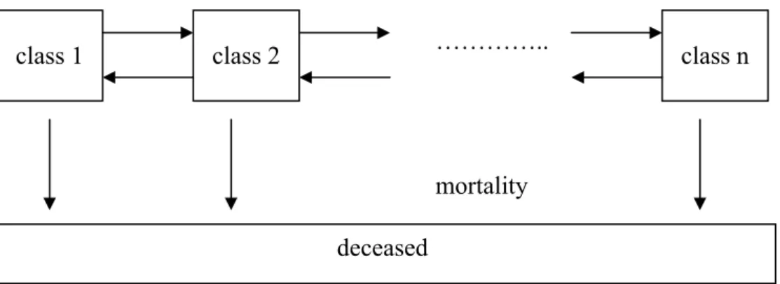
In Figure 5 and Figure 6 we present the general state-transition structure for any risk factor and disease respectively.
Figure 5 presents the state-transitions for any risk factor. The horizontal arrows describe the transitions between the risk factor classes for those that survive, the vertical arrows describe the transition to the state ‘deceased’, i.e. mortality. For instance, for the risk factor smoking, the classes are never smokers, smokers and former smokers and n equals 3. Arrows from class 1 to class 2 and class 2 to class 2 represent smoking initialization and smoking cessation, an arrow from class 3 to class 2 represents relapse, while from class 2 back to class 1 no arrow exists, since
returning to the class of never smokers is not possible. In the figure only transitions between neighboring classes were shown for graphical simplicity, but this is no restriction to the model. In case of treatment, additional classes and transitions may be introduced.
…………..
mortality
Figure 5: Transitions between risk factor classes and mortality
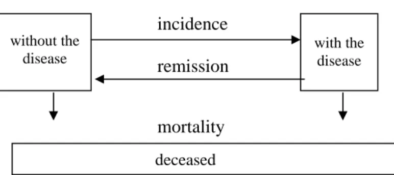
Figure 6 presents the state-transition structure for any disease. We distinguished only one disease condition here, i.e. with the disease. In principle, the mathematical model
class 1 class 2 class n
can deal with any number of disease states. The horizontal arrows describe the transitions between the states, i.e. disease incidence from the state ‘without the disease’ to ‘with the disease’. The vertical arrows describe the transition to the state ‘deceased’, i.e. mortality. Remission is the possibility to return from a disease state to a state without the disease. Disease incidence and as a result also disease mortality rates depend on the risk factor prevalences.
incidence remission
mortality
Figure 6: Transitions between disease states and mortality
Summarizing, Figure 7 shows all possible transitions in a time step ∆t with ncr(r) denoting the number of risk factor classes for risk factor r.
time t small change in time ∆t time t+∆t
gender g no changes ≡ g
age a aging= ∆t = a + ∆t
risicofactor r transitions between classes
classes 1 to ncr(r) classes 1 to ncr(r)
disease d transitions between states
not present not present
present present
alive mortality
yes yes
no no
Figure 7: Summary of possible transitions
with the disease without the
disease
The main assumptions that were used to formalize the joint CDM model versions are: (1) We assumed the individual life courses to be statistically independent
conditional on all covariates, i.e. the risk factor classes and disease conditions. In other words, all individuals behave independently given their
epidemiological characteristics.
(2) We assumed that all risk factors and chronic diseases have a discrete distribution. For continuous risk factors cut-off points were introduced to define a set of disjoint classes.
(3) We assumed the initial risk factor class prevalence rates independent. The initial disease prevalence rates were assumed independent conditional on these risk factors and on causally related intermediate diseases (‘local independence assumption’). In the CDM2003 marginal model version the class transition rates for each risk factor were also assumed to be independent from the other risk factors and the disease states. The CDM2005 joint version allowed us to condition the class transition rates on the disease state. For example, new cases of other CHD among current smokers may have higher cessation rates than CHD-free current smokers.
(4) The incidence rates for each disease were assumed to be independent from the other diseases, conditional on the risk factor levels and the causally related intermediate diseases (‘local independence assumption’). For example, the incidence rates for CVA and for other CHD were assumed independent conditional on the epidemiologic risk factors and the diabetes state. We included the most important joint risk factors in the model to cover the dependency relations between these diseases.
(5) We assumed that for any disease the excess mortality is independent from the risk factor levels. This means that the risk factors affect the disease prognosis only through increased risks for other diseases and mortality from other causes of death.
(6) We assumed that the disease-specific excess mortality rates are additive. The latter assumption of additive excess mortality rates was based on the additive cause-specific mortality hazard model.28
(7) We assumed multiplicative incidence and mortality risks, i.e. with no interaction on the log-linear scale. For example, the risk for incidence of Diabetes for an individual with both a high BMI and a low activity level is the multiplication of the risk rates for BMI and activity.
(8) The other causes mortality rates depend on the risk factors, but conditional on the risk factors do not depend on the disease states. That is, the risk to die of an accident is the same for a person with or without diabetes, conditional on risk factors.
(9) The risk rate for the incidence of diseases is an approximation for the risk rate for the prevalence of diseases. This assumption is used to derive some of the formulas below.
3.2
The new model of diabetes and macrovasculair
complications in relation to risk factors: input data
Here, the type of input data used is shortly described. The following inputdata were estimated, with inputdata new for CDM2005 joint version in bold:
• For each disease, prevalences in the model startyear, incidence rates and remission (for example for asthma) and mortality rates.
• For each risk factor, its division into classes, prevalences in the model startyear for each risk factor class, and transition rates between these classes (e.g. start and stop smoking).
• For each combination of a risk factor with a disease, per risk factor class the relative risks for incidence of the disease.
• For each combination of a causal disease with an ‘end’ disease, relative risks for incidence of the ‘end’ disease.
• Start prevalences in a diabetes population, for each risk factor distinguished
• Transition rates between classes in a diabetes population for each risk factor distinguished,
• Relative risks for risk factors in a diabetes population for incidence of macrovascular diseases.
The report ‘Modelling Chronic Diseases: the diabetes module. Justification of (new) input data in the mathematical RIVM Model’ 29 documents updates of the data that were already present in CDM2003, as well as the estimates used for the new model parameters listed above. All data must be age- and sex specific. Transition,
prevalence, incidence and mortality data need to apply to the Dutch population, and were therefore based on the most appropriate, recent Dutch registry data. Relations between risk factors and diseases (relative risks) were assumed to be less country specific and estimated from the international literature.
3.2.1 Population numbers
Demographic input data in CDM are from Statistics Netherlands. 30 The most important input data are the Dutch population numbers in the start year, divided into age and gender, prognosed numbers of births in each year, prognosed migration numbers, and all cause mortality specific to age and gender.
3.2.2 Prevalence of DM and riskfactors in startyear
In the joint model, prevalence has to be specified according to risk factors for complications. These joint prevalences can be computed based on relative risks and total prevalences (see 3.3.1.6). However, for diabetes, specific empirical data were also gathered for the most important risk factors, to validate the model computations. These empirical data were estimated for each risk factor separately, because the estimation of joint classess of all risk factors would result in unreliable estimates.
The importance of the inclusion of a riskfactors follows from: • its impact on complications
• available evidence on interventions for this risk factor • prevalence of the risk factor in the Dutch DM population
For the following risk factors additional empirical data were gathered : • total cholesterol
• systolic Bloodpressure • body Mass Index • physical activity • smoking
• level of HbA1c
For all these risk factors except HbA1c, both the prevalence in the total population as well the prevalence in the DM population was estimated. For HbA1c, only the prevalence in the DM population was estimated.
3.2.3 Transitions in a year
DM incidence
Total diabetes incidence was modelled as the weighted average of the different risk factor and disease classes using relative risks (see section 3.3.1.7). After incidence in DM, the new cases also have to be distributed over the DM risk factor classes.
For the risk factors that affect the incidence of diabetes, the relative risks for incidence of diabetes used in the model will influence the distribution of diabetes incidence over the risk factor classes. This is the case for:
• body mass index • physical activity • smoking
For the risk factors that do not affect DM incidence, incidence in DM will be
according to the prevalence in the total population. An adjustmentstep (see 3.3.1.7) is needed to adjust this incidence to the prevalence distribution of the risk factor in DM. This is the case for:
• total cholesterol • systolic Bloodpressure
Finally, the level of HbA1c is not modelled in the total population, mainly due to a lack of data, and hence the level of glycemic control in the incidence of diabetes will be an input parameter and was estimated from empirical data.
Transitions between risk factor classes.
This refers to transitions from e.g. low bloodpressure to higher bloodpressure, for the following risk factors:
• total cholesterol • systolic Bloodpressure • body Mass Index • physical activity • smoking
In the CDM2005 joint version, transition rates between risk factor classes for a certain risk factor were assumed equal for all combinations of joint states that reflect a
transition between these classes. That is, the smoking cessation rate is the same in people with and without diabetes and with a high or a low Body Mass Index. From empirical data, transition rates for specific groups, for example, for diabetes patients could be estimated. Furthermore, if interventions affect these transition rates, they will differ between groups that receive an intervention and those without. Therefore, the model was structured such that transition rates can be adjusted for each specific joint state. For HbA1c, the transition rates were estimated for the diabetes population.
Mortality
Unadjusted excess mortality rates were estimated for DM, and its complications: AMI, other CHD, CVA and CHF. The excess mortality rates were then adjusted as described in section 3.3.1.4, based on the comorbidity rates as computed in section 3.3.1.3.
3.2.4 Relative risks
The incidence of the DM complications (AMI, other CHD, CVA and CHF) in the DM population as well as the incidence of these diseases in the general population without DM is linked to risk factor classes trough relative risks. These relative risks were adjusted for other, confounding factors included in the model to prevent double counting see sections 3.3.1.21 and 2.
Total incidence of complications was estimated from empirical data. Relative risks of the risk factors BMI and activity on DM incidence were used to distribute total incidence over different risk factor classes in the general population.
Furthermore, relative risks for incidence of AMI, other CHD, CHF and CVA in the general population were estimated, as well as the relative risks of intermediate diseases on ‘end’ diseases, for instance, the risk of diabetes on AMI.
3.2.5 Costs of care for each disease stage
An estimate of total costs of diabetes care has to include the costs related to
complications. We estimated Dutch costs for diabetes, based on data from the 1999 Cost of Illness in the Netherlands.
However, to analyze the effect of interventions on costs of care, it is relevant to distinguish between cost of care for diabetes alone and costs related to complications which may be prevented by the interventions. To obtain this, we excluded the costs of modeled complications from the total cost estimate and used the model instead, including costs of care for cardiovascular diseases to estimate these costs directly. Because the same relative risk estimates were used in the cost of diabetes estimate and in the model, for a current practice scenario, the model computes the same total diabetes costs.
If hypothetical scenarios would be computed with free interventions which reduce rates of cardiovascular complications, then total diabetes costs will decrease. Of course, interventions are not free, so that this decrease must then be corrected for the costs of the intervention.
Ideally we also want to divide the costs of diabetes without costs of cardiovascular complications over the different classes of HbA1c level. This will then allow
analyzing interventions which result in better control of the level of HbA1c for their consequences on costs of care for diabetes.
3.2.6 Quality of life in each disease stage
The Chronic Disease Model uses estimates from the Global Burden of Disease Study and its Dutch Counterpart 4 31-34 to attribute loss of quality of life weights to diseases.
For Diabetes, these weights will be further specified for the different classes of HbA1c level. The effect of the presence of macro vascular complications is modeled through comorbidity. To compute the quality of life in joint states with different diseases present, an assumption has to be made about how comorbidity affects quality of life. Three possible assumptions are that the quality of life weight for a state with both disease A and B could be 1) the lowest of the weights for A or B, 2) the
multiplication of the two weights, or 3) the addition of the two weights. These three assumptions were analyzed and their results were compared. This is reported in detail in the report on the health economics module.16 In the CDM2005 joint version, it is possible to choose among the three different assumptions.
3.3
Methodological issues in a diabetes model, formal
solutions in CDM2005 joint version
To start the formal description of the model structure, the variables available as input data in the model will be listed. Let d= A,B,C,D,… denote the nd diseases in the model. Let r=R,S,… denote the nrd risk factors in the model, each with risk factor classes i=1,..,ncr(r ). All variables used were age and gender specific, but for ease of notation, these arguments will be ignored below. Then, input data for the model are: emd disease d excess mortality rate
mtot all cause mortality rates pd disease d prevalence rates incd disease d incidence rates
cfd disease d case fatality rate, i.e. the 1-month mortality rate after
disease onset
remd disease d remission rates
pri class i prevalence rate for risk factor r
λr
ij transition rates between risk factor classes, for each risk factor r and all
classes i,j
RRri,tot the relative risk for total mortality for risk class i of risk factor r
RRrd,i (unadj) the relative risk in risk class i of risk factor r for incidence of disease d, unadjusted for intermediate diseases
RRd, A (unadj) the disease A relative risk for incidence of disease d unadjusted for
intermediate diseases
The values for the transition rates and prevalence rates were estimated from empirical data, while the relative risks were estimated based on analyses of data obtained from literature reviews. For diabetes, more detailed estimates were available on risk factor prevalence and on the relative risks for incidence of complications.29
Given the input variables, in the model initialization steps the variables needed at the start of the simulation are calculated.
3.3.1 Model initialization steps
At model initialization, the following steps are taken:
1. adjust incidence risk rates of one disease on another for intermediate diseases 2. adjust incidence risk rates of risk factors on diseases for intermediate diseases 3. calculate co-morbidity prevalence rates
4. adjust excess mortality rates for double-counting mortality numbers 5. calculate mortality for other causes
6. compute prevalence rates in joint risk factor and disease classes 7. calculate incidence rates for all model states
3.3.1.1 Adjustment of co-morbidity disease incidence risks for intermediate diseases
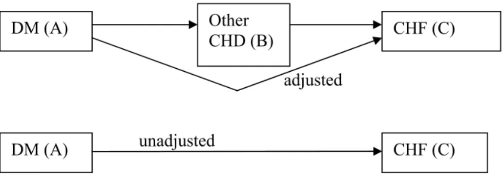
For each pair of successively causally related diseases we adjusted the incidence risk rates of one disease on another for the intermediate disease. For example (see Figure 6), the relative risks of DM on CHF are adjusted for other CHD being an intermediate disease between DM and CHF.
adjusted
unadjusted
Figure 8: Example of complication risks also working through intermediate disease
We derived the unadjusted relative risk of DM on CHF by rewriting the unadjusted risk rate, conditioning on the intermediate disease other CHD, i.e. as a function of the adjusted relative risk (see appendix B). The resulting formula was then rewritten to express the adjusted relative risk as the unadjusted risk times an adjustment factor: RRC,A = RRC,A(unadj) *
{1+(RRB,A – 1) pA+(RRC,B – 1) pB}/{1+(RRB,A –1) pA+(RRC,B –1)RRB,A pB}
with:
RRC,A the disease C relative risk for disease A, that is the relative risk for
individuals with A to get C, adjusted for intermediate disease B. RRC,A(unadj) the disease C relative risk for disease A unadjusted for intermediate
disease B
RRB,A the disease B relative risk for disease A
RRC,B the disease C relative risk for disease B
DM (A) Other
CHD (B) CHF (C)
pA, pB the prevalence rate for disease A and B respectively
The formula shows that the adjustment depends on the prevalence rates of both the causal disease (A) and the intermediate disease (B), and the relative risks of all causal relations involved. The smaller the disease B prevalence rate, the smaller the
adjustment.
In the extreme case of pB = 0, the formula reads RRC,A = RRC,A(unadj)*{1+(RRB,A–1)
pA}/{1+(RRB,A –1) pA}= RRC,A(unadj) and the adjustment has no effect. Another
example is the case that disease A is no risk factor for B (RRB,A = 1). Then, the
formula reads: RRC,A =RRC,A(unadj) *{1 + (RRC,B –1) pB}/{1 +(RRC,B – 1)*1*pB}=
RRC,A(unadj).
For more complex relations between diseases, like those shown in Figure 1, the adjustment has to take place for all relations respectively.16 This calculation method is possible as long as the causally related disease pairs constitute a so called directed a-cyclic graph. That means, if one disease works as an intermediate disease for another, the latter one is no intermediate disease for the former. Assessing the a-cyclic graph of causally related diseases is a graph-theoretical problem, and has been solved using the so-called adjacency matrix of causally related disease pairs. That is, referring to Figure 1, all dependency relations around diabetes were formalized in a square matrix with a separate row/column for each disease. This matrix contains a ‘1’ if the disease in the column is caused by the disease in the row and a zero otherwise. Then the matrix was reordered so that it formed an upper diagonal matrix. From this matrix, the order of the dependency relations forming an acyclic graph could be obtained. For the structure in Figure 1 the following ordered list of pairs of diseases results:
{{DM, other CHD},{other CHD, AMI},{AMI,CHF},{DM, AMI},{other CHD,CHF} ,{DM,CHF}}.
The adjustment is done going trough this list from the beginning to the end. That is, first the RR of DM on AMI is adjusted for other CHD, then the RR of other CHD on CHF is adjusted for AMI, and finally the RR of DM on CHF is adjusted for AMI.
3.3.1.2 Adjusting disease incidence risks of risk factors for intermediate diseases
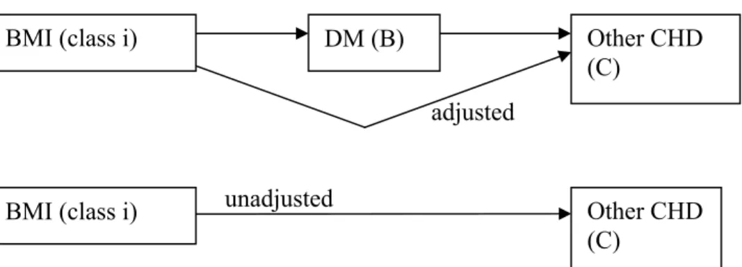
For each pair of causally related diseases the epidemiological risk factors affect the dependent ‘end’ disease in two ways, directly as well as indirectly through the
independent ‘causal’ disease. For example, (see Figure 9) the dependent ‘end’ disease other CHD incidence risk depends on the prevalence rate of the intermediate disease DM for any risk factor class of the risk factor BMI.
adjusted
unadjusted
Figure 9: Adjustment of (other CHD) relative risks for risk factors for intermediate disease (DM)
Note the similarity to Figure 6 above. Analogously to the adjustment of relative risks of one disease on another, the unadjusted relative risk can be rewritten as the adjusted relative risk times a factor (see appendix B). Rewriting this formula then expresses the adjusted relative risk as the unadjusted risk times an adjustment factor:
RRrC,i = RRrC,i(unadj) *
{ E(RRr B) + (RRC,B – 1) pB }/ { 1 + (RRC,B–1) (RRrB,i –1) pB}
with:
RRrC,i disease C incidence relative risk for risk factor class i adjusted for
intermediate disease B
RRrC,i(unadj) disease C incidence relative risk for risk factor class i unadjusted for
intermediate disease B
RRrB,i disease B incidence relative risk for risk factor class i
E(RRrB) mean value of disease B relative risk over all classes of risk factor r
RRC,B disease C incidence relative risk for disease B adjusted for risk
factor
pB disease B prevalence rate
This formula is analogous to the formula in subsection 3.3.1.1. To see this, note that that for diseases, the E(RRB), that is, the mean value of RR B,A over all classes (states)
of the causal disease A equals pA*RR B,A+ (1- pA)* 1= (RR B,A-1)* pA +1.
Again, the calculation method is possible as long as the causally related disease pairs constitute a directed a-cyclic graph.16 The formula was then applied recursively, that is going from the beginning to the end along the list of all ordered pairs of related diseases. For example, at first the relative risks of for instance the risk factor BMI on other CHD were adjusted for the intermediate disease DM, then those of BMI on AMI for the intermediate diseases DM and other CHD, etcetera.
BMI (class i) DM (B) Other CHD
(C)
BMI (class i) Other CHD
3.3.1.3 Calculation of initial disease co-morbidity rates
Using the relative risks mentioned in the foregoing paragraph, we calculated the initial prevalence rates for all co-morbidity disease states. The calculation steps applied were the following.35
(1) We calculated the co-morbidity prevalence risks resulting from joint risk factors using the relative risk values for these risk factors. For example, smoking as a joint risk factor results in co-morbidity of other CHD and lung cancer. We used the assumptions of independently distributed risk factors and multiplicative risks: pA,B = Πr Σi RRrA,i RRrB,i pri pA pB / ( Πr Σi RRrA,i pri * Πr Σi RRrB,i pri )
with:
pA , pB prevalence rate of disease A and B respectively
pA,B joint prevalence ( = co-morbidity) rate of both diseases A and B
RRrA,i, RRrB,i relative risk of disease A and B respectively for class i of risk
factor r
pri prevalence rate of class i of risk factor r
The formula shows how the disease co-morbidity rate depends on the risk factors through the relative risks. If one disease is not associated with any risk factor (the relative risks have value 1 for all r), the co-morbidity rate is equal to the product of the disease prevalence rates and the diseases are independently distributed.
(2) We adjusted the co-morbidity prevalence risks for all causally related disease pairs using the empirically known disease incidence risks adjusted for intermediate diseases (see 3.3.1.1). For example, DM as an independent risk factor for CHF results in co-morbidity between DM and CHF.
(3) We adjusted the co-morbidity prevalence risks for joint intermediate diseases. For example, co-morbidity between DM and CHF also results from the effect of DM on CHF through the intermediate disease AMI.
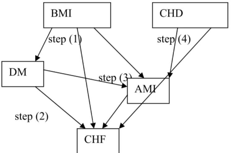
(4) We adjusted the co-morbidity prevalence risks for joint ‘causal’ diseases. For example, co-morbidity between AMI and CHF results from other CHD (Angina Pectoris) being an independent risk factor for both AMI and CHF.
(5) Finally, since all co-morbidity risks were defined as prevalence rate ratios we calculated for each causally related pair of diseases the co-morbidity rate ratio for the reversed pair. For example, the prevalence rate ratio for other CHD given disease CHF was calculated from the prevalence rate ratio for CHF given other CHD.
step (1) step (4)
step (3)
step (2)
Figure 10: Example of steps to calculate co-morbidity rates
These calculation steps result in co-morbidity prevalence rate ratios for each pair of diseases that are related through joint risk factors and/or directly or indirectly through intermediate diseases along a pathways of causal relations.
If empirical data are available on the comorbidity prevalence rates then an alternative approach is to use these empirical estimates.
3.3.1.4 Adjustment of excess mortality rates
CDM distinguishes two types of disease-related mortality: (1) mortality with the disease, and (2) mortality due to the disease. The model parameter related to (1) is the excess mortality rate, i.e. the excess mortality rate of persons with the disease
compared to those without the disease. The excess mortality rates can also be caused by other co-morbid chronic diseases such as disease complications, e.g. other CHD being a complication of diabetes. Summing up excess mortality numbers over all diseases then results in double-counting mortality cases. Therefore we also need (2), the adjusted disease-related excess mortality rates. These excess mortality rates are adjusted for competing death risks, and thus can be interpreted as the mortality uniquely attributable to the disease. Unadjusted disease-related excess mortality rates can be estimated from empirical data.29 36 37 We calculated the excess mortality rates from empirical disease incidence and prevalence rates available from registries in general practice using the DisMod model equations.38 The DisMod equations express the relation between disease incidence, prevalence and mortality rates. They allow computing one of these rates from data on the other two.
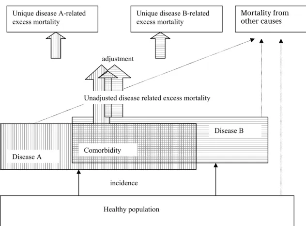
Figure 11 presents all cause mortality, disease-related mortality, and mortality from other causes of death in relation to co-morbidity.
BMI
CHF
AMI DM
Figure 11: Relation between all cause and disease-related mortality
The co-morbidity prevalence rates were calculated in the foregoing paragraph (3.3.1.3). Using these co-morbidity prevalence rates we related the unadjusted disease-related excess mortality to the adjusted ones (see appendix C for details)39: emA = emA0 + { Σd≠A ( pd,A - pA pd)/pA(1-pA ) }emA0
with:
emA, emA0 disease A excess mortality rate unadjusted and adjusted for co-morbidity respectively
pd, pA disease d and disease A prevalence rate
pd,A joint prevalence (= co-morbidity) rate of diseases d and A The term ( pd,A - pA pd) is the calculated morbidity prevalence rate minus the co-morbidity rate found in case of independent disease rates. The term pA(1-pA ) is used to scale the expression and equals pA,A - pA pA , the ‘co-morbidity of a disease with itself’ (note that pA,A= pA ). Combining these equations for all diseases result in a matrix equation:
diag(M) {em} = M {em0}
Healthy population incidence Disease A Disease B Comorbidity Mortality from other causes Unique disease A-related
excess mortality
Unique disease B-related excess mortality
adjustment
with:
M matrix with elements ( pd,A - pA pd).
diag(M) the diagonal-matrix of M , that is, the matrix with elements pA(1- pA) {em}, {em0} vector of excess mortality rates unadjusted and adjusted
respectively The matrix equation was solved: {em0} = M-1 diag(M) {em}
In this way the empirically known unadjusted excess mortality rates were adjusted for double-counting mortality numbers through co-morbidity.
3.3.1.5 Mortality rates and rate ratios for other causes
The all cause mortality rates are the sum of the adjusted excess mortality rates and the mortality rates from other causes of death. All cause mortality numbers are available from Statistics Netherlands (CBS). The adjusted disease-related excess mortality rates were calculated above. We combined both to calculate the mortality rates for other causes of death. We took account of the ‘acute’ mortality of diseases, i.e. the 1-month mortality (case fatality) rate immediately after disease onset. This type of mortality was modeled only for diseases with unstable initial disease periods, i.e. AMI and CVA:
moc = mtot - Σd emd0 pd - Σd incd cfd
with:
moc mortality rate for other causes of death mtot all cause mortality rate
pd disease d prevalence rates
emd0 disease d excess mortality rates adjusted for co-morbidity incd disease d incidence rate
cfd disease d case fatality rate, i.e. the 1-month mortality rate after
disease onset
Likewise we calculated the relative risks for other causes of death, i.e. the relative mortality risks through all diseases that were not included in our model. The equations are expressed in so called risk multipliers, these are re-scaled relative risks, obtained by dividing the relative risk with the weighted average of relative risks over all risk classes.40
RMr
i,oc ={ RMri,tot mtot – Σd RMrd,i [emd0 pd + incd cfd ] } / moc with the same notation as above and:
RMri,oc = RRri,oc / Σi RRri,oc pri risk multiplier for other causes of death for class i of risk factor r
RMri,tot = RRri,tot / Σi RRri,tot pri risk multiplier for all cause mortality
RMrd,i= RRrd,i / Σi RRrd,i pri risk multiplier for disease d incidence in risk class i of risk factor r.
pri class i prevalence rate for risk factor r
These equations may be solved for the RRr i,oc .
3.3.1.6 Initial prevalence rates for all model states
Next the initial prevalence rates for all joint states have to be calculated. That is, sthe prevalence rates for each value of the vector (i,j,…nrd,A,B,…nd) have to be determined. This vector represents a joint state and its first elements express risk factor class for each risk factor r=1,…nrd, while its the last elements express disease state (with the disease=1, without the disease=0) for each disease d=A,B,..nd.
In principle, the state prevalences could be based on empirical data. In practice, the available data will be less detailed. Therefore, the model also enables to approximate the joint prevalence rates from total disease prevalence and total risk factor prevalence rates in combination with relative risks. If more detailed input data are available, these may be used instead.
The initial class prevalence rates of the CDM2005 joint version were calculated in successive steps. We illustrate the results with an example on two risk factors with two classes each and two diseases.
(1) We calculated the prevalence rates for all joint risk factor classes. In case of two risk factors the class prevalence rates generate a two-dimensional table.
Table 1: Class prevalence and marginal prevalence in case of two risk factors
risk factor 2 marginal
class 1 class 2
risk factor 1 class 1 p11 p12 p11
class2 p21 p22 p12
marginal p2
1 p22
with:
pij prevalence rate for class i for risk factor 1 and class j for risk factor 2 pri class i prevalence rate for risk factor r
By applying assumption 3 of independent risk factor distributions we find: pij = p1i p2j
That means, the joint risk factor class prevalence rate is the product of the class prevalence rates. This first step can be written in general terms of any number of risk factors selected:
p0( r ) = Πr pri
with:
r vector of classes i for all risk factors r distinguished pri class i prevalence rate for risk factor r
p0( r ) joint prevalence rate of state r
(2) We multiplied these prevalence rates with the disease state prevalence rates applying the assumption of independent disease distributions conditional on the risk