Renewable energy sources

Hele tekst

(1)

(2) ON THE GLOBAL AND REGIONAL POTENTIAL OF RENEWABLE ENERGY SOURCES Over het mondiale en regionale potentieel van hernieuwbare energiebronnen (met een samenvatting in het Nederlands). PROEFSCHRIFT TER VERKRIJGING VAN DE GRAAD VAN DOCTOR AAN DE UNIVERSITEIT UTRECHT OP GEZAG VAN DE RECTOR MAGNIFICUS,. PROF. DR. W.H. GISPEN, INGEVOLGE HET BESLUIT VAN HET COLLEGE VOOR PROMOTIES IN HET OPENBAAR TE VERDEDIGEN OP VRIJDAG 12 MAART 2004 DES MIDDAGS OM 12.45 UUR. door. Monique Maria Hoogwijk geboren op 22 november 1974 te Enschede.

(3) Promotor: Prof. Dr. W.C. Turkenburg Verbonden aan de Faculteit Scheikunde van de Universiteit Utrecht Promotor: Prof. Dr. H.J.M. de Vries Verbonden aan de Faculteit Scheikunde van de Universiteit Utrecht. Dit proefschrift werd mede mogelijk gemaakt met financiële steun van het Rijksinstituut voor Volksgezondheid en Milieu (RIVM).. CIP GEGEVENS KONINKLIJKE BIBLIOTHEEK, DEN HAAG. Hoogwijk, Monique M. On the global and regional potential of renewable energy sources/ Monique Hoogwijk – Utrecht: Universiteit Utrecht, Faculteit Scheikunde Proefschrift Universiteit Utrecht. Met lit. opg. − Met samenvatting in het Nederlands ISBN: 90-393-3640-7 Omslagfoto: NASA Omslag ontwerp: Dirk-Jan Treffers en Monique Hoogwijk, met dank aan Jacco Farla.

(4) ON THE GLOBAL AND REGIONAL POTENTIAL OF RENEWABLE ENERGY SOURCES. Aan mijn ouders.

(5) CONTENTS Chapter one: Introduction 1. Energy and sustainable development. 9 9. 2. Future energy scenarios 2.1 Scenarios on future energy system and energy models 2.2 The SRES scenarios. 11 11 13. 3. The potential of wind, solar and biomass energy. 16. 4. Renewable electricity in the IMAGE/TIMER 1.0 model 4.1 The IMAGE/TIMER 1.0 model 4.2 Restriction to wind, solar PV and biomass electricity 4.3 The electricity simulation in TIMER 1.0. 17 17 18 19. 5. Central research question. 20. 6. Outline of this thesis. 22. Chapter two: Exploration of the ranges of the global potential of biomass for energy. 25. 1. Introduction. 26. 2. Methodology 2.1 Biomass categories 2.2 Approach. 27 27 29. 3. The potential for energy farming on agricultural land 3.1 Availability of surplus agricultural land (Category I) 3.2 Availability of marginal/degraded land for energy farming (Category II) 3.3 Productivity and primary energy potential of energy crops 3.4 Summary of the potential of energy crops. 29 29 33 34 35. 4. The potential supply of biomass residues 4.1 Agricultural residues (Category III) 4.2 Forest residues (Category IV) 4.3 Animal residues (Category V) 4.4 Organic waste (Category VI). 36 36 36 37 37. 5. Bio-material production (Category VII). 37. 6. Integration and discussion 6.1 Integration 6.2 Discussion. 39 39 40. 7. Conclusions. 41. Chapter three: Potential of biomass energy under four land-use scenarios. Part A: the geographical and technical potential. 43. 1. Introduction. 44. 2. Definitions and system boundaries 2.1 Categories of potentials 2.2 Description of primary biomass categories 2.3 Restriction to woody energy crops 2.4 Restriction of conversion technologies.. 46 46 47 48 49. 3. Methodology, framework, scenarios and main assumptions. 49.

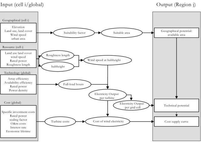
(6) 3.1 The IMAGE 2.2 model: the Terrestrial Environment System (TES) 3.2 The quantification of the SRES Scenarios of the IPCC 3.3 Land availability (Ai): different categories of land for energy plantations 3.4 The land-claim exclusion factor 3.5 The management factor for energy crops. 51 54 56 57 60. 4. Results for land availability and energy crop productivity 4.1 Land availability 4.2 The productivity of energy crops. 61 61 65. 5. Results for the theoretical and geographical potential 5.1 The theoretical potential of biomass energy 5.2 The global geographical potential of energy crops 5.3 Regional variation in geographical potential. 67 67 67 68. 6. The technical potential of biomass energy. 72. 7. Sensitivity analysis and discussion 7.1 Sensitivity of the available area from abandoned agricultural land 7.2 Comparison of the geographical potential with previous studies 7.3 Discussion of results. 73 73 77 79. 8. Summary and conclusion. 80. Chapter four: Potential of biomass energy under four land-use scenarios. Part B: exploration of regional and global cost-supply curves. 85. 1. Introduction. 86. 2. Methodology 2.1 Crop choice and land-use scenarios 2.2 The cost-supply curve of primary biomass energy from energy crops 2.3 The cost-supply of secondary biomass: liquid fuel and bio-electricity. 87 87 88 93. 3. Inputs to assess the production cost of energy crops 3.1 Land productivity and geographical potential 3.2 Land rental cost 3.3 Capital, labour cost, substitution coefficient and learning 3.4 Transportation cost 3.5 Conversion to liquid fuel and bioelectricity. 95 95 97 98 99 100. 4. The cost-supply curves of primary biomass energy. 102. 5. The cost-supply curve of secondary biomass energy. 107. 6. Sensitivity analysis. 108. 7. Discussion 7.1 Comparison with other studies 7.2 Limitations of this study. 111 111 112. 8. Summary and conclusion. 113. Chapter five: Assessment of the global and regional technical and economic potential of onshore wind-energy 117 1. Introduction. 118. 2. Approach and definitions. 120. 3. Theoretical potential. 121.

(7) 4. The geographical potential. 122. 5. The technical potential 5.1 Wind regime 5.2 Wind turbine output; amount of full-load hours 5.3 Wind power density per km2 5.4 Results. 127 127 129 130 132. 6. The cost of wind electricity: the economic potential using regional cost supply curves 6.1 Approach 6.2 Results. 134 134 135. 7. Discussion of the results 7.1 Sensitivity analysis 7.2 Comparison with previous studies 7.3 Discussion of main assumptions. 137 137 141 143. 8. Conclusions. 145. List of variables. 146. Chapter six: Assessment of the global and regional technical and economic potential of 149 photovoltaic energy 1. Introduction. 150. 2. Approach 2.1 System definitions and boundaries 2.2 Definition of potential. 152 152 154. 3. Theoretical potential: the solar radiation. 155. 4. The geographical potential. 158. 4.1 Suitable area. 158. 4.2 Results on the geographical potential. 163. 5. The technical potential 5.1 How to estimate the technical potential 5.2 Results of the technical potential assessment. 164 164 165. 6. The economic potential of PV electricity 6.1 The cost of PV electricity 6.2 The cost of PV electricity and the PV cost-supply curve. 166 166 167. 7. Future perspective of PV electricity. 170. 8. Sensitivity analysis. 172. 9. Discussion. 176. 10. Summary and conclusions. 178. List of variables. 181. Chapter seven: Exploring the impact on cost and electricity production of high penetration levels of intermittent electricity in OECD Europe and the USA. 185. 1. Introduction. 186. 2. Regional static cost-supply curves of wind and solar PV. 188. 3. Factors determining the overall production cost of wind and solar PV in the electricity system 3.1 Additional cost factors with increasing penetration levels. 192 193.

(8) 3.2 Related aspects for the overall cost development of intermittent electricity 3.3 Technological learning: declining capital costs. 195 197. 4. Simulation of wind/solar PV penetration: the use of the TIMER-EPG model 4.1 General description of TIMER-EPG 4.2 Investment strategy 4.3 Electricity demand 4.4 Spinning reserve and back-up capacity 4.5 Supply and cost of conventional electricity 4.6 Supply of wind and solar PV electricity 4.7 Discarded wind and solar PV electricity 4.8 Operational strategy 4.9 Technological learning: declining capital costs. 197 197 198 199 200 200 201 202 202 203. 5. Results 5.1 Intermittent electricity production and load factor (Experiment A) 5.2 Discarded electricity from intermittent sources (Experiment A) 5.3 Costs of wind electricity (Experiment A) 5.4 Fuel savings (Experiment B) 5.5 Potential CO2 abatement costs (Experiment B). 203 203 205 207 209 210. 6. Sensitivity analysis (Experiment B). 212. 7. Discussion. 214. 8. Summary and conclusions. 217. Chapter eight: Summary and conclusions. 221. Chapter eight: Samenvatting en conclusies. 231. References. 242. Dankwoord. 254. Curriculum Vitae. 256.

(9)

(10) CHAPTER ONE INTRODUCTION 1. Energy and sustainable development Energy plays a crucial role in the development of economies and their people. The energy system, considered as the whole of the energy supply sector, which converts the primary energy to energy carriers, and the end-use technologies needed to convert these energy carriers to deliver the demanded energy services (see Figure 1), has developed significantly over time. Two main transitions can be distinguished in the history of the energy system (Grübler et al., 1995; Grübler, 1998). The first was the transition from wood to coal in the industrialising countries, initiated by the steam engine in the late 18th century. The use of coal, which could more easily be transported and stored, allowed higher power densities and related services to be site independent. By the turn of the 20th century nearly all primary energy in industrialised countries was supplied by coal. The second transition was related to the proliferation of electricity, resulting in a diversification of both energy enduse technologies and energy supply sources. Electricity was the first energy carrier that could easily be converted to light, heat or work at the point of end use. Furthermore, the introduction of the internal combustion engine increased mobility, as cars, buses and aircraft were built, and stimulated the use of oil for transportation. These innovations together lead to a shift in the mix of commercial energy sources from mainly coal towards domination of coal, oil and later natural gas and increased the global commercial primary energy use from 1850 to 1990 by a factor of about 40 (Grübler, 1998). However, the energy system has developed differently over the world. At present we are living in a world where about 4 billion people use mainly fossil fuels as their primary energy sources and rely for about 16% on electricity for their energy services, whereas about 2.4 billion people rely for most of their energy supply on traditional fuels and energy sources, such as biomass (IEA/OECD, 2002a). As the latter consumption corresponds to only about 11% of the total primary energy use, it is not directly visible and often neglected in statistics on energy consumption (Goldemberg, 2000). This disparity in the availability of energy services reflects the disparity in possibilities for (economic) development. For that reason energy plays a crucial direct or indirect role in order to achieve several Millennium Development Goals (MDGs) constructed at the Millennium Summit held in 2000 at the United Nations General Assembly (Goldemberg 9.

(11) CHAPTER ONE. and Johansson, to be published). Consequently, in the debates at the World Summit on Sustainable Development (WSSD) in Johannesburg held in September 2002, energy was one of the key issues. It was concluded that the current use and production of energy carriers is incompatible with the goal of sustainable development in view of the following (Goldemberg and Johansson, to be published): • Opportunities for economic development are constrained for more than two billion people that do not have access to affordable energy services. • Social stability is threatened due to a growing disparity in access to affordable energy. • Human health, regional and local air pollution and ecosystems are threatened due to energy-related emissions like suspended fine particles and precursors of acid deposition. • There is increasing evidence that the anthropogenic greenhouse gas (GHG) emissions originating from the combustion of fossil fuels and unsustainable use of biomass energy have a severe impact on the climate system. • As economies rely for a significant part on imported energy, they are also increasingly vulnerable to disruption in the supply. Energy supply system Primary energy. Coal. Solar. Conversion technology. Combustion power plant. Solar thermal cell. Wind turbine. Secondary energy. Electricity. Heat. Electricity. Transportation. Grid. Grid. Grid. Final energy. Electricity. Heat. Electricity. End-use conversion technology. Lamp. Boiler. Cook-stove. Hair dryer. End-use energy. Light. Hot water. Heat. Heat. End-use Technology system. Room. District heating grid. Pan. Energy service. Lighting a room. Warming a house. Cooking food. Fuelwood. Wind. Drying hair. Energy end-use system. Figure 1: Description of the energy system consisting of the energy supply and end-use system and four examples of energy systems (based on de Beer, 1998). One of the pathways to follow in order to achieve the goals of sustainable development is an increased reliance on renewable energy. Renewable energy conversion technologies (‘renewables’) generally depend on energy flows through the earth‘s ecosystem fed by 10.

(12) INTRODUCTION. solar radiation and the geothermal energy of the earth (Turkenburg, 2000). A major advantage is that they can be extracted in a ‘renewable’ mode, i.e. their rate of extraction is lower than the rate at which new energy is arriving or flowing into the reservoirs (Sørensen, 2000). Renewables are expected to be suitable alternatives in a sustainable energy future for several reasons (Turkenburg, 2000): • They lead to a diversification of energy sources by increasing the share of a diverse mixture of renewable sources, and thus to an enhanced energy security. • They are more widely available compared to fossil fuels and therefore reduce the geopolitical dependency of countries as well as minimise spending on imported fuels. • They contribute less to local air pollution (except for some biomass applications) and therefore reduce the human health damages. • Many renewable energy technologies are well suited to small-scale off-grid applications and hence can contribute to improved access of energy services in rural areas. • They can balance the use of fossil fuels and save these for other applications and future use. • They can improve the development of local economies and create jobs. • They do not give rise to greenhouse gas (GHG) emissions to the atmosphere. This also holds for the use of biomass, if produced in a sustainable way, as the emitted carbon has been produced before in the process of photosynthesis. Biomass energy can then be considered as carbon dioxide neutral. 2. Future energy scenarios For the reasons mentioned above, e.g. energy security, accessibility to affordable energy services, energy related emissions to the atmosphere, etc., it is interesting to assess the potential supply of renewables to long-term energy demand at a global scale. Since several decades, the possible developments and dynamics of the energy system is analysed at various levels of geographical detail. These studies give insight in energy security at the long term, in the rate the resources may be depleted, in how the energy prices may develop, and in possible developments of energy-related emissions to the atmosphere. Amongst others this type of analyses facilitates the international policy debate regarding climate change. To assess the future energy consumption and supply mix, assumptions on technical, demographical, economic, social, institutional and political parameters have to be made. To study these issues in a consistent manner, a scenario approach is usually adopted. 2.1 Scenarios on future energy system and energy models Scenarios are images of possible alternatives for the future. They are neither predictions nor forecasts, but are consistent descriptions of how the future may unfold (Grübler et al., 1995), (Nakicenovic, 2000). One of the first global energy scenarios has been. 11.

(13) CHAPTER ONE. constructed at the International Institute of Applied System Analysis (IIASA) during the late 1970s. Since then a large number of global energy scenarios have been developed. Two types of scenarios on the future energy system can be distinguished: descriptive scenarios, and normative scenarios. The first type gives insights in possible pathways for the future; the latter explores the future routes that can be taken to end at a certain predefined end-point. Some typical normative scenarios developed in the context of sustainable development are (Goldemberg et al., 1988), RIGES (Renewable Intensive Global Energy Supply) (Johansson et al., 1993), and the Fossil Free Energy Scenario (FFES) scenario developed by the Stockholm Environmental Institute in collaboration with Greenpeace (1993) (Lazarus, 1993). Typical descriptive scenarios are the emission scenarios that have been developed in the context of the Intergovernmental Panel on Climate Change (IPCC), like the most recent so-called SRES scenarios (Special Report on Emission Scenarios) (Nakicenovic, 2000). Main driving forces of the scenarios that influence the future energy system are: • population dynamics; • economic dynamics; • technological change; • social dynamics. Population dynamics influence the demand side of the energy system. Economic development affects the demand as well as the availability of the energy resources or the supply mix, as it is a measure for the future availability of financial resources for investments in the energy supply sector. Technological change is reflected in the demand for energy, e.g. through technological improvements on energy efficiency, as well as on the supply side, e.g. through conversion technologies that come available, specific investment costs and limits to up-scaling. These driving forces need to be consistent within a scenario and are quantified within a modelling framework. For that reason, scenarios are often characterised by the development paths of the driving forces described above. Scenarios on the future energy system can be quantified by using energy models. Energy models are widely used by national governments and international agencies to aid the decision-making process, e.g. regarding energy and environmental policies, prospects of future technologies and energy supply strategies (Audus, 2000). One can distinguish various types of energy models, e.g. regarding their geographical coverage (e.g. national versus global), their timeframe (e.g. a year versus a century), their number of energy carriers and sectors included in the model and the main approach that is used for the calculation (e.g. optimisation towards cost or deterministic simulation model). Examples of energy models that compute the global long-term energy system are the MESSAGE model (Messner and Schrattenholzer, 2000), the POLES model (Criqui, 1996), the 12.

(14) INTRODUCTION. MERGE model (Manne et al., 1995) and the IMAGE/TIMER1.0 model (de Vries et al., 2002). These models are linked to sub-models that amongst others include the GHG emissions that are related to the conversion of primary energy to other energy carriers and the final use of these carriers. The demand for energy services is estimated and from there, via conversion and end-use technologies efficiencies, the required primary energy can be computed. The type of primary energy sources that is used is mostly determined by the operational cost and performance of the final energy. 2.2 The SRES scenarios Recently developed descriptive scenarios are the SRES scenarios from the IPCC (Nakicenovic, 2000). Their aim is to simulate the long-term (up to 2100) greenhouse gas emissions due to the combustion of fossil fuels. These scenarios are based on four storylines that describe how the world could develop over time. Differences between the scenarios concern the economic, demographical and technological development and the orientation towards economic, social and ecological values. The four storylines are constructed along two axes, (see Figure 2). The A1 and A2 storylines are considered societies with a strong focus towards to economy, economic development. Whereas the B1 and B2 storylines are more focused on welfare issues and are ecological orientated. The A1 and B1 storylines are globally oriented, with a strong focus towards trade and global markets. A2 and B2 are more oriented towards regions. These storylines are the origin of a large set of scenarios. Figure 3 describes the energy mixture and the total energy demand of the four marker1 scenarios from the IPCC. In all scenarios biomass and renewable energy sources, mainly solar energy and wind energy, are expected to contribute at significant levels.. The marker scenarios were originally posted in draft form on the SRES website to represent a given scenario family. The choice of the marker was based on which of the initial quantification best reflected the storyline, and the features of specific models.. 1. 13.

(15) CHAPTER ONE Material/economic. A1. A2. Population: 2050: 2100:. 8.7 billion 7.1 billion. Population: 2050: 2100:. 11.3 billion 15.1 billion. GDP:. 24.2 • 103 billion $95 y-1 86.2 • 103 billion $95 y-1. GDP:. 8.6 • 103 billion $95 y-1 17.9 • 103 billion $95 y-1. 2050: 2100:. 2050: 2100:. Technological growth: high. Technological growth: low. Trade: maximal. Trade: minimal. Regional oriented. Global oriented. B1. B2. Population: 2050: 2100:. 8.7 billion 7.1 billion. Population: 2050: 9.4 billion 2100: 10.4 billion. GDP:. 18.4 • 103 billion $95 y-1 53.9 • 103 billion $95 y-1. GDP:. 2050: 2100:. 2050: 2100:. 13.6 • 103 billion $95 y-1 27.7 • 103 billion $95 y-1. Technological growth: high. Technological growth: low. Trade: high. Trade: low. Environment/Social. Figure 2: Description of the main four storylines from SRES (for reference, see text).. 14.

(16) INTRODUCTION Economic/material A2 Marker (ASF). A1 Marker (AIM). 1600 1400. 2200 2000. -1. ). 1800. 2400. Other renewables Biomass Nuclear Gas Oil Coal. Total primary energy consumption (EJ y. ). 2000. -1. 2200. Total primary energy consumption (EJ y. 2400. 1200 1000 800 600 400 200 0 1990 2000 2010 2020 2030 2040 2050 2060 2070 2080 2090 2100. 1800 1600 1400. Other renewables Biomass Nuclear Gas Oil Coal. 1200 1000 800 600 400 200 0 1990 2000. Globalisation. 2010 2020 2030. B1 Marker (IMAGE 2.1). 1600 1400. 2400. 1200 1000 800 600 400 200 0 1990. 2000. 2010. 2200 2000. -1. Other renewables Biomass Non-fossil electric Gas Oil Coal. ). 1800. 2020. 2030. 2040. 2050. 2060 2070 2080. 2090 2100. Regionalisation. B2 Marker (MESSAGE). Total primary energy consumption (EJ y. ). 2000. -1. 2200. Total primary energy consumption (EJ y. 2400. 2040 2050. 2060. 2070. 2080. 2090. 2100. 1800 1600 1400. Other renewables Biomass Nuclear Gas Oil Coal. 1200 1000 800 600 400 200 0 1990 2000 2010 2020 2030 2040 2050 2060 2070 2080 2090 2100. Environmental/social. Figure 3: The simulation of the energy mixture and total primary energy demand over time for the four SRES marker-scenarios of the IPCC (Nakicenovic, 2000). In parenthesis, the name of the energy model is given. From Figure 3 it can be seen that due to the variation in the population dynamics, and the economic and technological development, the various scenarios of the future energy system show large differences, both regarding the total demand, as well as the mixture of the used primary energy sources. Regarding the latter, most studies simulate a significant contribution of ‘renewable energy sources’ in the future, although among scenarios and among modelling frameworks the quantitative estimated of their market share varies considerably. Variation also consists when the same storyline is used (Nakicenovic, 2000). What are the reasons for these variations? A variety of questions or driving sources are conceptualised differently in the different scenarios. One of them is how prices of fossil fuels will evolve. When and how the transition to more costly variants – such as tar sands and oil shales – will occur and whether and how political (in)stabilities will affect prices is quite uncertain. Then, 15.

(17) CHAPTER ONE. although most analysts would agree that the large cost reductions of wind turbines and solar photovoltaic in the last decades will continue, there are controversial views on the rate at which this will or can happen, and hence on the penetration rate of these technologies. Moreover, there are the large uncertainties on costs and land requirements for large-scale production of commercial biomass energy, and on the interference with food production and climate change. Compounding these uncertainties are the prospects and problems of novel end-use technologies and carriers such as fuel cells and hydrogen. It is increasingly recognized that the answers to these questions are not merely a matter of cost and technology; also societal developments such as life-styles, the role of market institutions and the balance between decentralized and centralized options are important aspects. The considerations put forward to explain the differences in the results for the different scenario analyses shown in Figure 3 emphasize the importance of the use of a set of scenarios that are well-chosen, well-described and sufficiently transparent to show the impact of the separated input parameters. Important input parameters are the potential availability of the separate energy sources and the developments of the conversion technologies and the associated production costs. This thesis therefore focuses on the cost-supply curves of wind, solar PV and biomass energy. As such, insight is gained in the main input parameters of energy scenarios. 3. The potential of wind, solar and biomass energy The main characteristic of renewable energy sources is that they can be extracted in a ‘renewable’ mode. Wind, solar and biomass energy are all derived from the sun which, when considered at timeframes of centuries, supplies a constant flow of energy to the earth. The potential availability of wind, solar and biomass energy over time and between regions is therefore hardly varied by the resource availability (theoretical limit), but rather by geographical developments, e.g. land-use demands, by technical developments, e.g. innovative conversion technologies, economic developments, e.g. labour cost variations, or implementation constraints, (e.g. legislations). These aspects vary the potential availability over time and among regions. When studying the potential of (renewable) energy sources, the aspects like geographical, technical and economic developments need consideration. As a result, different types of potentials can be defined, e.g. the categories introduced by van Wijk and Coelingh (1993): • The theoretical potential is the theoretical limit of the primary resource. For solardriven sources this is the solar energy or solar energy converted to wind or biomass. • The geographical potential is the theoretical potential reduced by the energy generated at areas that are considered available and suitable for this production.. 16.

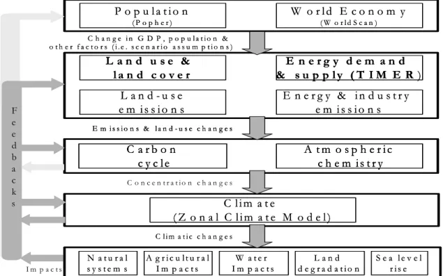
(18) INTRODUCTION. • The technical potential is the geographical potential reduced by the losses of the conversion of the primary energy to secondary energy sources • The economic potential is the total amount of technical potential derived at cost levels that are competitive with alternative energy applications. • The implementation potential is the total amount of the technical potential that is implemented in the energy system. Subsidies and other policy incentives can give an extra push to the implementation potential, but social barriers like noxious smell can reduce the implementation potential. The implementation potential can be both higher and lower then the economic potential, but can never exceed the technical potential. In the literature, there are various studies that assess the potential of wind energy (Grubb and Meyer, 1993; World Energy Council, 1994; Fellows, 2000; Sørensen, 1999; Rogner, 2000); solar energy (Hofman et al., 2002; Sørensen, 1999; Rogner, 2000); or biomass energy (Berndes et al., 2003; Rogner, 2000) at a global scale. The studies show that for each of the sources, the potential availability is significant and exceeds the present electricity consumption. However the above-presented distinction between the different types of potentials is in these studies mostly not made, except for the assessment of the potential fo wind energy, formulated by Utrecht University and presented by the World Energy Council (1994). Moreover, most studies, except World Energy Council (1994), Fellows (2000) and Hofman et al. (2002), do not include the production cost, or the economic potential of renewable resources. In addition, most studies, neglect the impact on the operational costs if intermittent sources of wind or solar PV electricity penetrate the electricity system. For biomass energy it is concluded that no potential assessment has been conducted with the use of different land-use scenarios. Finally, the studies differ according to their regional aggregation and approach. Therefore no comparison could be made between the categories of potentials for the three renewable energy sources at similar regional aggregation. In this thesis, the theoretical, geographical, technical and economic potential of wind, solar PV and biomass energy is assessed, using a similar approach. As such, not only more insight is gained in the factors that influence the availability; the types of potentials can also be better compared among the energy sources. 4. Renewable electricity in the IMAGE/TIMER 1.0 model 4.1 The IMAGE/TIMER 1.0 model In this thesis we focus on the energy model IMAGE/TIMER 1.0, or simply TIMER 1.0 (de Vries et al., 2002). The TIMER 1.0 model is a system-dynamic, simulation model of the global energy system at an intermediate level of aggregation. TIMER 1.0 is a submodel of the IMAGE 2.2 model (Integrated Model to Assess the Global Environment) (IMAGEteam, 2001) (Figure 4). The IMAGE 2.2 model is developed at grid cell level of 0.5° x 0.5° (longitude, latitude). It is also this level that is mainly used in this thesis. All results of IMAGE 2.2, TIMER 1.0 and this thesis are aggregated to 17 world-regions: 17.

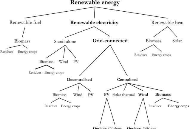
(19) CHAPTER ONE. Canada, USA, Central America, South America, Northern Africa, Eastern Africa, Western Africa, Southern Africa, OECD Europe, Eastern Europe Former USSR, Middle East, South Asia, East Asia, South East Asia, Oceania, Japan. TIMER 1.0 distinguished itself from top-down or optimisation models using a combination of bottom-up engineering information and specific rules and mechanisms about investment behaviour and technology development to simulate the possible development and characteristics of the energy system over time. TIMER 1.0 aims to analyse the long-term dynamics of energy conservation and use and the transition to nonfossil fuel use within an integrated modelling framework, and to calculate energy related greenhouse gases emissions, which are used as an input in other sub-models of IMAGE 2.2. The competition among energy sources within the TIMER 1.0 model is based on long-term cost-supply curves per energy technology and the technical potential of supply per technology and energy source. P o p u la tio n. W o r ld E c o n o m y. (P o p h e r). (W o r ld S c a n ). C h a n g e in G D P , p o p u la tio n & o t h e r f a c t o r s ( i.e . s c e n a r io a s s u m p t io n s ). L an d u se & la n d c o v e r. E n e rg y d e m a n d & s u p p ly ( T I M E R ). L a n d -u se e m is s io n s. FF ee ee d d b ba ac ck ks s. E n e r g y & in d u s tr y e m is s io n s. E m is s io n s & la n d - u s e c h a n g e s. C arb o n c y c le. A tm o s p h e r ic c h e m is tr y. C o n c e n tr a tio n c h a n g e s. C lim a te (Z o n a l C lim a te M o d e l) C lim a tic c h a n g e s. Im p a c ts. N a tu ra l sy ste m s. A g r ic u ltu r a l Im p a c ts. W a te r Im p a c ts. L and d e g r a d a tio n. S e a le v e l r is e. Figure 4: Framework of the IMAGE 2.2 models and the connection with the energy demand and supply model TIMER 1.0 (source: IMAGEteam, 2001). 4.2 Restriction to wind, solar PV and biomass electricity We focus ourselves on renewable electricity only. This has been done because electricity is increasingly used in the energy system. It is widely applicable but cannot be stored at short and longer timeframes in large quantities. Wind, solar and biomass energy can all be converted to electricity. They are included in one sub-model of the TIMER 1.0 model. It is therefore rather easy to implement the results of the assessment of the potential of these sources in the TIMER 1.0 model. The restriction to electricity only means that we exclude the production of heat and fuel using renewables. Furthermore, we focus on grid18.

(20) INTRODUCTION. connected applications since, in terms of quantities involved, these are most significant in the energy system and are only included in TIMER 1.0. The renewables that are included in this thesis are shown in Figure 5 in bold, we also mention the options and technologies that are not investigated.. Renewable energy Renewable fuel. Renewable electricity. Biomass Residues. Renewable heat. Grid-connected. Stand-alone. Energy crops. Biomass Residues. Biomass. Wind. Solar. Energy crops. PV. Residues Energy crops. Decentralised Biomass. Wind. Centralised. PV. PV Solar thermal Wind. Residues Energy crops. Biomass Residues. Onshore Offshore. Energy crops. Onshore Offshore. Figure 5: The types of renewable energy carriers and technologies that are included in this thesis (in bold). 4.3 The electricity simulation in TIMER 1.0 TIMER 1.0 consists of various sub-models. The Electric Power Generation (EPG) submodel focuses on the overall long-term dynamics of regional electricity production. The model can be summarised in two parts (Figure 6). The first part is the investment strategy, which simulates the investments in various forms of electricity production in response to a demand for expansion and for replacement capacity. The investment strategy is based on changes in relative fuel prices and changes in relative generation costs of thermal and non-thermal power plants. The second part simulates the operational strategy. The operational strategy determines how much of the installed capacity is used and when. It reflects that electric power companies minimise the production costs while maintaining the required system reliability. The basic rule-of-thumb here is the merit order strategy: power plants are operated in order of variable costs. Technological learning is included using exogeneous assumptions and using an experience curve for the renewable energy sources, resulting in a decrease of the operational costs. Depletion is included using a cost-supply curve resulting in an increase of operational costs.. 19.

(21) CHAPTER ONE Population Existing park. Technology Electricity demand. Lifetim e plants D em and for replacem ent capacity. D em and for capacity M ultinom inal logit M arket shares. Cost of conventional electricity Cost of interm ittent electricity. + learning - depletion Investment strategy. Load dem and curve N ew Park Operational strategy Fuel use. CO 2 em issions. Figure 6: Schematic description of the TIMER 1.0 model. The current version of TIMER 1.0 simulates renewable electricity sources in an aggregated manner. To enhance the detail of TIMER 1.0 these sources should be simulated separately. Therefore, similar main input (cost-supply curve) per source and technology is required, at similar regional aggregation and timeframe (1970 to 2050 and/or 2100). In this thesis we construct cost-supply curves of wind, solar PV and biomass electricity that can be used for scenario simulation in the TIMER 1.0 model. We also analyse in this thesis how the intermittent sources wind and solar PV can be implemented in the TIMER 1.0 model and how this would influence the cost of wind electricity and the CO2 abatement costs. 5. Central research question In the above sections we have addressed the importance of analysing the theoretical, geographical, technical, economic and implementation potential of wind, solar PV and biomass electricity in a consistent way. We also have indicated the importance of studying the renewable electricity sources, in particular wind and solar PV in the context of an energy model. The main objective of this thesis is: To assess the geographical, technical and economic potential of wind, solar and biomass electricity for seventeen world regions by constructing regional cost-supply curves for these renewable electricity options using a grid cell approach. In addition, we aim to investigate the dynamics and main factors that influence the additional overall production and CO2 abatement costs of intermittent sources with increasing penetration in the electricity market. 20.

(22) INTRODUCTION. To analyse this objective, relatively more attention is given to biomass energy. This is done the feedstock availability depends on the land-use system development over time (Berndes et al., 2003). Furthermore, the costs of biomass energy are more regionally varying, so more regional detail is needed to analyse the regional cost-supply curves of biomass energy. The objective of this thesis is reached by addressing the following research questions: • What range can be expected of the geographical potential of biomass energy? • What factors determine the geographical potential of biomass energy? • What is the geographical and technical potential of biomass energy for four different land-use scenarios? • What are the regional cost-supply curves and the economic potential of biomass energy? • What is the geographical, technical and economic potential of onshore wind electricity? • What is the geographical, technical and economic potential of onshore solar PV electricity? • What factors influence the amount of wind and solar PV electricity absorbed by the electricity system? • How do the operational costs of wind electricity change with increasing penetration levels? • What factors determine the CO2 abatement costs of wind electricity at increasing penetration levels of wind in the electricity system? To meet the objective we will assess the theoretical, geographical and technical potential of wind, solar PV and biomass electricity in this thesis. This has been done using climatic and land-use data at grid-cell level of 0.5°x 0.5° (except for Chapter 2). This geographical aggregation level is consistent with the level used in the terrestrial environment system of the IMAGE 2.2 model. The results are aggregated to the regional level of the TIMER 1.0 model. For the biomass energy potential assessment we will use four land-use scenarios as the assessment of the availability of biomass energy requires an integrated approach with land-use development. The cost-supply curves at a regional and global level are derived by calculating the electricity production costs in each grid cell. These include the costs of the fuel (zero for wind and solar PV), specific investment costs and the operation and maintenance costs. These grid cells are ranked according to their production costs resulting in the cost-supply curve.. 21.

(23) CHAPTER ONE. 6. Outline of this thesis This thesis is structured as follows. Chapter 2 starts with an exploration of the ranges of the geographical potential of biomass energy. This study identifies the factors that determine the long-term geographical potential of biomass energy. In Chapter 3 a similar approach is used to assess the regional geographical and technical potential of energy crops based on four land-use scenarios. These potentials are used in Chapter 4 to estimate the long-term development of regional cost-supply curves of energy crops within the four assumed scenarios. The following chapters focus on the potential supply and cost-supply curves of wind and solar PV electricity. In Chapter 5 the theoretical, geographcial and technical potential of wind electricity and cost-supply curves of onshore wind electricity production is estimated on the basis of a static land-use pattern. A similar study is presented in Chapter 6 for solar PV. In Chapter 7 the TIMER-EPG model is used to simulate the impact of high penetration levels of wind and solar PV on the amount of intermittent electricity in the system, the overall production and CO2 abatement costs of wind electricity in the USA and OECD Europe. The final Chapter 8 summarises the main findings and conclusions of this thesis.. 22.

(24) ART BIOMASS ENERGY.

(25)

(26) CHAPTER TWO. EXPLORATION OF THE RANGES OF THE GLOBAL POTENTIAL OF BIOMASS FOR ENERGY#. Abstract This study explores the range of the future global potential of primary biomass energy. The focus has been put on factors that influence the potential biomass availability for energy purposes rather than give exact numbers. Six biomass resource categories for energy are identified: energy crops on surplus cropland, energy crops on degraded land, agricultural residues, forest residues, animal manure and organic wastes. Furthermore, specific attention is paid to the competing biomass use for material. The analysis makes use of a wide variety of existing studies on all separate resource categories. The main conclusion of the study is that the range of the global potential of primary biomass (in about 50 years) is very broad, quantified at 0 – 1135 EJ y-1. Energy crops from surplus agricultural land have the largest potential contribution (0 – 988 EJ y-1). Crucial factors determining biomass availability for energy are: 1. The future demand for food, determined by population growth and future diet; 2. The type of food production systems that can be adopted world-wide over the next 50 years; 3. Productivity of forest and energy crops; 4. The (increased) use of bio-materials; 5. Availability of degraded land; 6. Competing land use types, e.g. surplus agricultural land used for reforestation. It is therefore not ‘a given’ that biomass for energy can become available at a large-scale. Furthermore, it is shown that policies aiming for the energy supply from biomass should take factors like food production system developments into account in comprehensive development schemes. #. Published in Biomass and Bioenergy (2003), Vol. 25, Issue 2, pp: 119-133. Co-authors are André Faaij, Richard van den Broek, Göran Berndes, Dolf Gielen and Wim Turkenburg. Joep Luyten is kindly thanked for his support of Section 4. The authors furthermore are grateful to Eric Kreileman (RIVM) for his help on Figure 2. This work has been conducted with financial help of the Netherlands Agency for Energy and the Environmental (NOVEM)..

(27) CHAPTER TWO. 1. Introduction Biomass is seen as an interesting energy source for several reasons. The main reason is that bioenergy can contribute to sustainable development (van den Broek, 2000). Biomass energy is also interesting from an energy security perspective. Resources are often locally available and conversion into secondary energy carriers is feasible without high capital investments. Moreover, biomass energy can have a positive effect on degraded land by adding organic matter to the soil. Furthermore, biomass energy can play an important role in reducing greenhouse gas emissions, since if produced and utilised in a sustainable way, the use of biomass for energy offsets fossil fuel greenhouse gas emissions. Since energy plantations may also create new employment opportunities in rural areas in developing countries, it also contributes to the social aspect of sustainability. At present, biomass is mainly used as a traditional fuel (e.g. fuelwood, dung), globally contributing to about 45 ± 10 EJ y-1. Modern biomass (e.g. fuel, electricity) to about 7 EJy-1 (Turkenburg, 2000). In this study we include both traditional and modern biomass energy. Many energy scenarios suggest large shares of biomass in the future energy system e.g. (Nakicenovic, 2000; Shell, 1995; Johansson et al., 1993; Goldemberg, 2000). The availability of this biomass is not always separately analysed. Furthermore, large-scale utilisation will have large consequences for land demand and biomass infrastructure, which should be assessed. Many studies have been undertaken to assess the future primary biomass energy potential, e.g.: (Battjes, 1994; Dessus et al., 1992; Edmonds et al., 1996; Fischer and Schrattenholzer, 2001; Grübler et al., 1995; Hall et al., 1993; Lashof and Tirpak, 1990; Lazarus, 1993; Leemans et al., 1996; Rogner, 2000; Shell, 1995; Swisher and Wilson, 1993; Williams, 1995; World Energy Council, 1994; Yamamoto et al., 1999). To get insight in the main assumptions that have been made in these studies Berndes et al. (2003) have conducted an analysis of the approaches used to assess the global biomass energy potential. Overall, it has been concluded that the results vary widely. Furthermore, most of the investigated studies do not include all sources of biomass in competition with other land use functions. The studies are not always transparent in the procedure for calculating the energy potential. Insight in factors that are of main importance to realise the investigated potential is therefore not always presented. Finally, many studies tend to neglect competition between various land use functions and between various applications of biomass residues (Berndes et al., 2003). Therefore, in this study we consider a different approach of exploring the primary biomass potential. The main objectives of this study are: 1) to gain insight in factors that influences the primary potential of primary biomass for energy in the long term; 2) To explore the theoretical ranges of the biomass energy potential on the longer term in a comprehensive way, including all key categories and factors; 3) To evaluate to what extent the potential of 26.

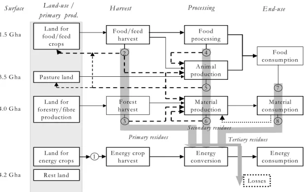
(28) EXPLORATION OF RANGES OF POTENTIAL OF BIOMASS ENERGY. biomass supply can be influenced. This analysis focuses on a global scale. The chosen timeframe for this exercise is the year 2050. In this study we first describe the methodology applied (Section 2). Next, in Sections 3 and 4 the potential production of biomass is assessed. In Section 5, the potential future demand of biomass for production of materials as a competing option is taken into account by evaluation of utilisation, and potential growth in demand for the long term with the use of economic projections. Finally, the ranges found for land availability, biomass productivity levels, availability of biomass residues and of organic wastes are translated into primary energy supply potentials (Sections 6 and 7). 2. Methodology 2.1 Biomass categories First we define the concept ‘potential’ that is used in this study. We are interested in an upper limit of the amount of biomass that can become available as (primary) energy supply without affecting the supply for food crops. This is defined as the geographical potential. We define our biomass supply system by dividing biomass production and use into different resource categories (Figure 1). These categories increase transparency in competition and synergy of separated biomass resources. The scheme presented in Figure 1 is a simplification of the real system, and hence not complete. E.g. one could think of aquatic biomass from the fresh water or oceans. Furthermore, the land use category ‘other land’ includes all kind of land types such as desert, semi-arid land, ice, etc. This scheme also implies that biomass supply from protected nature conservation areas is not included in this study. Competing land use functions like recreation and human settlements are also excluded. Nevertheless, residues from forest areas are included in this study. Figure 1 also shows the total surface per land use type. Out of the total land surface of 13 Gha, about 5 Gha is used for food production (Wirsenius, 2000). To some extent the figures vary among different studies, e.g. Fischer and Schrattenholzer (2001) take a figure of 5.3 Gha.. 27.

(29) CHAPTER TWO Surface. 1.5 G ha. Land-use / primary prod.. Harvest. Land for food/feed crops. Food/feed harvest. End-use. Food processing Food consum ption. 4. 2. 3.5 G ha. Processing. Anim al production. Pasture land. 5 4.0 G ha. Forest harvest. Land for forestry/fibre production. M aterial production. 4.2 G ha. Rest land. 1. M aterial consum ption. 6 Secondary residues. 3 Primary residues. Land for energy crops. 7. Energy crop harvest. 8. Tertiary residues Energy conversion. Energy consum ption Losses. Figure 1: Overview of competition and synergism among various types of biomass flows and the global land surface. Based on: (van den Broek, 2000 and Wirsenius, 2000). The black arrows indicate the main product flows, whereas the dotted lines show potential non-energy applications of various residue categories. The gray arrows represent the potential energetic use of the resources (1 = energy crops, 2 = energy crops at degraded land, 3 = agricultural residues, 4 = forest residues, 5 = animal manure, 6 = organic waste, 7 = bio-material). In the system defined (Figure 1) there is on the one hand competition for land, for the production of energy, food and materials; i.e. farmers may compete with foresters or energy producers on the use of land for their products. Furthermore, competition exists between the use of residues (dotted lines). Residues can be used for energy purposes, but also for fiber, fertiliser or fodder. On the other hand, synergies occur between energy and food material production (the end-use options, right part of the figure), since residue flows increase with increasing food production and these flows can also be utilized for energy purposes. To explore the ranges of biomass potential for energy that includes all those flows and applications we define -based on Figure 1- seven categories of biomass resource types (Table I). Land for energy crops from Figure 1 is divided in two categories (here referred to as categories I and II): surplus agricultural land and degraded land. Degraded land is included in the land use category ‘other land’ in Figure 1. The primary and secondary residues, as shown in Figure 1, are estimated separated, but merged due to lack of detailed disaggregated data. This is done for both agricultural residues (Category III) and forest residues (Category IV). The use of biomass for material applications (such as solid products or fiber or wood for pulp) may increase in the future, and should be subtracted 28.

(30) EXPLORATION OF RANGES OF POTENTIAL OF BIOMASS ENERGY. from the biomass production for energy applications on surplus agricultural and degraded land. However, after a delay of time (which can cover a time period between several weeks (paper) up to decades (construction wood), this biomass becomes, at least partly, available as waste and adds to Category VI (organic waste). Table I: Biomass resource categories distinguished in this study to assess the global available potential of biomass for energy use on the long term. Category Category I: Biomass production on surplus agricultural land Category II: Biomass production on degraded land Category III: Agricultural residues Category IV: Forest residues (incl. material processing residues) Category V: Animal manure (dung) Category VI: Organic wastes Category VII: Bio-materials. Description The biomass that can be produced on surplus agricultural land, after the demand for food and fodder is satisfied. The biomass that can be produced on deforested or otherwise degraded or marginal land that is still suitable for reforestation. Residues released together with food production and processing (both primary and secondary). Residues released together with wood production and processing (both primary and secondary). Biomass from animal manure. Biomass released after material use, e.g. waste wood (producers), municipal solid waste. Biomass directly on used as a feedstock for material end-use options like pulp and paper, but also as feedstock for the petrochemical industry.. 2.2 Approach The potential supply of the various categories presented in Table I is assessed using the results of existing studies. For the assessment of biomass produced on surplus agricultural land (Category I), the demand for land required for food is assessed. Therefore various population scenarios, three different diets and two different food production systems are assumed. The potential of Category II is mainly based on an overview of studies with the objective to assess the amount of degraded land available for reforestation. The potential biomass productivity at both surplus agricultural and degraded land is estimated using a grid cell based crop growth model. The potential assessment of residues (Category III, IV, V and VI) is based on various potential assessments. The approaches are compared and similar assumptions and results combined to construct a lower and upper limit of the potential. The demand for bio-materials (Category VII) is based on scenarios on the future economic development, production figures and share of bio-materials in the total material production. The results of the separated categories are combined to give an overall estimation of the upper and lower ranges of primary biomass supply. 3. The potential for energy farming on agricultural land 3.1 Availability of surplus agricultural land (Category I) To assess land areas available for production of biomass for energy use on surplus agricultural land, the future demand for land for food and fodder production has to be 29.

(31) CHAPTER TWO. estimated. In order to do so, we use a study from Luyten that explores the potentials of food production on a global level (Luyten, 1995), as basis for the assessments. Several adaptations are made to the Luyten study, mainly regarding the land areas included. The adaptations can be done since the study by Luyten has been reported transparently. While Luyten considers all land that can be used in principle for food production (e.g. including current forests), we limit ourselves to the current 5 Gha in use for food production (see also Figure 1). At present, (forest) land is converted into agricultural land. And so, the agricultural land is increasing. If more land is required for food production, there is no land available for energy crops. We assume furthermore that the land area that is abandoned because of a decreased quality is included in the second category of biomass sources (energy crops on degraded land). The first category only includes (high quality) surplus agricultural land. Furthermore, more recent insights on population growth scenarios are used (Nakicenovic, 2000). We assess the potential future world food demand assuming three population projections and three food consumption patterns. To assess the required land to supply this demand, two types of food production systems are assumed, based on very different input levels of fertilisers and pesticides and more intensified management techniques and thus different intensities of farming (Luyten, 1995). Hence, eighteen different food scenarios are produced. 3.1.1 Future demand for food Total food demand depends primarily on population figures and the average diet consumed. Three average food consumption patterns are considered, taken from (Luyten, 1995): a vegetarian diet with little or no animal protein; a moderate diet; and an affluent diet with a large share of meat and dairy products (Table II). The diets are composed of different shares of plant, dairy and meat products. To make the diets comparable, they are expressed in grain equivalents (gr. eq.). Grain equivalents are universal measures for the amount of dry weight in grains used directly or indirectly (as raw material for other food products e.g. milk or meat) in our food consumption. In this approach some crops, which are not cereals (e.g. fruit) are translated to grains (Luyten, 1995). Losses when converting grains and grasses to dairy and meat products are taken into account. Luyten assumes conversion efficiencies of 33% for dairy and 11% for meat2. The three diets are all sufficient with respect to daily caloric intake and daily protein requirements, but differ strongly with respect to their composition and thus daily consumption per adult in grain equivalents (see Table II). The conversion factor that converts the diets to grain equivalents, are weighted averages of the conversion factors of each separate product consumed in the diet, respectively 0.92, 1.45 and 2.77 kg grain eq/kg product, for the vegetarian diet, moderate and affluent diet (Luyten, 1995). Taking into account an annual increase of productivity of about 2%, these data compare reasonably with present production efficiencies as studied by Wirsenius. Wirsenius mentions a variation of conversion efficiency from corn (in corn equivalents) between 5.2 and 19%, for cattle milk and dairy products respectively. For meat production a range is given of 0.58 – 1.8% for beef, 2.8 – 6.4% for pork meat, 4.1 – 8.3% for chicken and 10-18% for eggs (Wirsenius, 2000).. 2. 30.

(32) EXPLORATION OF RANGES OF POTENTIAL OF BIOMASS ENERGY. Table II: Assumed global average daily consumption per adult for three different diets expressed in MJ day-1 and in grain equivalents in kg dry weight per day, source: (Luyten, 1995). d-1). Energy intake (MJ Plant prod. (gr eq, kg-1d-1) Meat prod. (gr eq, kg-1 d-1) Dairy prod. (gr eq, kg-1d-1) Total (gr eq, kg-1d-1). Current situation 9.4. 2.3. Vegetarian diet 10.1 1.05 0.28 1.3. Moderate diet 10.1 0.90 0.22 1.23 2.4. Affluent diet 11.5 1.13 1.91 1.16 4.2. Population projections are taken from recent scenario studies of the Intergovernmental Panel on Climate Change (Nakicenovic, 2000). Projections for 2050 vary between 8.7 to 11.3 billion people, compared to the present (2000) figure of 5.9 billion global citizens. Combined with the three average diets described, and assuming that the entire world population adopts those diets, this results in the total future food demands for the three diets as indicated in Table III. Hence, it can be concluded that the total global demand (represented in grain equivalents) can, in principle, vary between 4.1 ⋅ 1012 and 17.3 ⋅ 1012 kg dry weight, which is 80% up to 350% of the current demand for food. Table III: Population projections for 2050 (in 109 people) and the food requirement in grain equivalents (in 1012 kg dry weight) for three population scenarios (L = low, M = medium and H = high). Current situation Population size 109 people 5. 9 Global food requirement 5.0 (1012 kg d.weight gr. eq.). Vegetarian diet L M H 8.7 9.4 11.3 4.1 4.5 5.4. Moderate diet L M H 8.7 9.4 11.3 7.6 8.2 9.9. Affluent diet L M H 8.7 9.4 11.3 13.3 14.4 17.3. 3.1.2 Future supply of food Two fundamentally different production systems are defined to assess the future supply of food: a High External Input (HEI) system and a Low External Input (LEI) system (Luyten, 1995). These systems differ mainly in the way diseases and plagues are combated and in the use of fertilisers. HEI production system The HEI production system is based on the concept of ‘best technical means’: crop production is maximized, and realized under optimum management, with an efficient use of resources (WRR, 1992 and Luyten, 1995). Nutrient requirements are fully covered by fertiliser application. The crop production is only limited by the availability of water if no irrigation water can be applied. The most effective methods of weed, pest and disease control are used to avoid yield losses and there are no restrictions in biocide use. Typical yields are 14.3 tons dry matter of gr. eq. ha-1y-1 for irrigated areas and 5.9 tons dry matter 31.

(33) CHAPTER TWO. of product in gr eq ha-1y-1, for non-irrigated areas (Luyten, 1995). These figures are relatively high (about a factor 2) compared to the present yield figures (2000) of cereal crops in Western Europe, of 5.7 ton ha-1y-1, and a world average figure of 3.1 ton ha-1y-1 (FAO, 2003). LEI production system The LEI system aims at an agricultural system that minimises environmental risks. Within this system, no chemical fertilisers and biocides are applied. Fertilisation is only obtained through biological fixation and is kept in the system by recycling animal and crop residues. Potassium and phosphorous availability to the crop are assumed optimal, but production is limited by both water and nitrogen availability. Herbicide application is replaced by mechanical weeding and the control of pests and diseases is carried out by means of prevention. This results in an average yield of 4.0 tons dry matter of gr eq ha-1y-1 for irrigated areas and 2.2 tons dry matter of product in gr eq ha-1y-1 (Luyten, 1995). These figures are close to present global average cereal yields of 3.1 ton ha-1y-1 (FAO, 2003). Luyten has calculated the rainfed crop production for the two systems with a simple crop growth model. Calculations are done for grid cells of 1º x 1º (with site-specific climate and soil conditions) over the globe (Luyten, 1995). We use the global mean irrigated and nonirrigated yields as assessed by Luyten and presented in Table IV3. The assessed yields are applied at the 5 Gha agricultural land, divided into grassland (3.5 Gha) and cropland (1.5 Gha) (see Table IV). We assume that with both systems, 20% of the agricultural land area is irrigated, and that on grassland no irrigation is applied4. Table IV: Potential area, potential yields and total potential food production. Area (Gha). Irrigated Rainfed Grassland Total. HEI 0.75 0.75 3.5 5.0. LEI 0.75 0.75 3.5 5.0. Global mean yield gr. eq. in ton ha-1y-1 HEI LEI 14.3 4.1 5.9 2.1 5.9 2.1. Potential production gr. eq. in Gton y-1 HEI LEI 10.7 3.1 4.4 1.6 20.5 7.4 35.6 12.0. 3.1.3 Future land requirement for food production The ratio between global food production and global food requirements (see Table V) is used to calculate the fractions of agricultural land needed for food production. It is assumed that the remaining fraction in principle can be used for the production of biomass for energy. The demand is only fulfilled under optimal infrastructure to match Luyten has used the following values for the Harvest Index (ratio between of harvested part and total crops), being representative for current major cereals: 0.4 (LEI, grain), 0.45 (HEI, grain), 0.7 (LEI, grass) and 0.6 (HEI, grass) (Luyten, 1995). 4 Currently 20% of the present arable land in developing countries and 13% in developed countries is irrigated. In 2030 the share of irrigated versus non-irrigated land in developing countries is estimated to be 22% (FAO, 2000). 3. 32.

(34) EXPLORATION OF RANGES OF POTENTIAL OF BIOMASS ENERGY. supply and demand. However, food production between years and regions may vary, and unequal income distribution may keep food inaccessible to the poor if food supply is limited. Furthermore various transportation and distribution losses require a higher production compared to the consumption. Therefore, we use a ratio of 2 to guarantee food self-sufficiency. This assumption is based on discussions among several experts (Luyten, 1995 and Luyten, 2001). It is stressed that this value is rather arbitrary, as it depends on a large set of factors (e.g. unequal spatial distribution of demand and supply, variation among years and losses in transport). The fraction of agricultural land that may be used for biomass production and the total area available for biomass production are given in Table V, Table VI and Table VII. Table V: Ratio between the potential global food production and global food requirement in 2050, calculated for two production systems (HEI and LEI) using three population scenarios (low, medium, high).. HEI LEI. Vegetarian diet Low Medium 7.7 7.1 2.7 2.5. High 5.9 2.1. Moderate diet Low Medium 4.2 3.9 1.5 1.3. High 3.2 11. Affluent diet Low Medium 2.4 2.2 0.8 0.8. High 1.8 0.6. Table VI: The area available for energy plantations agricultural land area using a food security factor of 2.. HEI LEI. Vegetarian diet Low Medium 3.7 3.6 1.3 1.0. High 3.3 0.2. Moderate diet Low Medium 2.6 2.4 -. High 1.9 -. Affluent diet Low Medium 0.8 0.5 -. High 0 -. Table VII: The fraction of the total global area available for energy plantations using a food security factor of 2.. HEI LEI. Vegetarian diet Low Medium 74% 72% 26% 20%. High 66% 3%. Moderate diet Low Medium 52% 48% -. High 38% -. Affluent diet Low Medium 16% 9% -. High 3% -. 3.2 Availability of marginal/degraded land for energy farming (Category II) To investigate the potential availability of marginal/degraded land for energy farming, we have analysed a selection of studies that assess land availability for forest-based climate change mitigation strategies (see Houghton, 1990; Houghton et al., 1991; Grainger, 1988; Hall et al., 1993; Lashof and Tirpak, 1990). The approach in these studies is first to identify areas where human activities have induced soil and/or vegetation degradation. The identified areas are subsequently evaluated in order to estimate availability for reforestation. In this context biomass energy plantations offer one of several possible land use options. Forest replenishment and agroforestry systems are alternative strategies for 33.

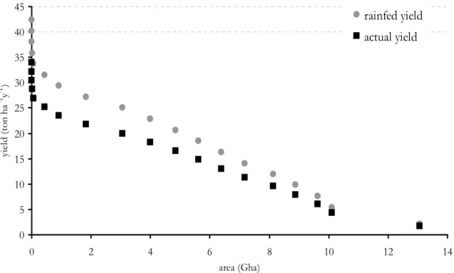
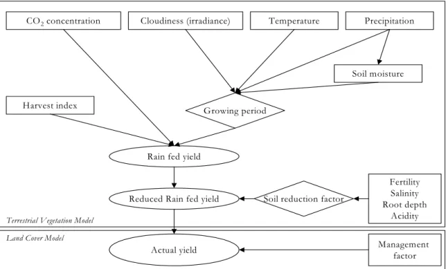
(35) CHAPTER TWO. reclamation of degraded land. The studies attempt to refine the reforestation concept in order to evaluate the feasibility for specific reforestation strategies. Otherwise, it is difficult to evaluate the feasibility of establishing biomass production for energy purposes on degraded land identified as potentially available for forestry based climate change mitigation strategies. The reason is that land availability assessments within the context of bioenergy plantations establishment require a more restricting set of evaluation criteria than if the assessment is employed within the context of forestation strategies in general. Hall et al. (1993) assumes that out of the 760 Mha of degraded land as mentioned by (Grainger, 1988), about 430 Mha can be used for energy crops. US-EPA (Lashof and Tirpak, 1990) assumes an amount of land available for reforestation of 380 Mha. Houghton (1990) and Houghton et al. (1991) estimates 500 – 580 Mha. However, a pessimistic scenario by (Houghton et al., 1991) gives a figure of 0 Mha. This pessimistic scenario was described to state that, due to financial, policy and social aspects, the effort for this deforestation could also be zero. However, as we do not include these aspects in this study, the range taken in this study, based on above-mentioned references is 430 – 580 Mha of degraded area potentially available for energy crop production. The lowest figure applies to the scenario when competing land use options are chosen. The upper limit assumes high priority input and marginal competing options. However, one should be aware that these figures are difficult to quantify, so these values are highly uncertain. 3.3 Productivity and primary energy potential of energy crops In this study the species of energy crop is not specified. For the productivity assessment we restrict the energy crop to woody short rotation crops, like eucalyptus and willow. Energy crop productivity depends on environmental conditions (i.e. climate, soil, etc.) and management (i.e. crop protection, nutrient supply, irrigation, etc.) and can therefore vary considerably among different areas. We distinguish two types of biomass cultivation for energy. The first type of cultivation is reforestation on degraded land, characterized by (more) extensive management and often on less productive land. The second category is ‘dedicated fuel supply systems’, with a more intensive management methods, (e.g. eucalyptus, grasses, willows). The latter is assumed to have a higher productivity. The value of this future productivity is difficult to assess, as well as the difference in productivity between both production systems. We have studied the productivity of energy crops, using the crop growth model of the IMAGE 2.1 model (see Figure 2). This crop growth model is similar to the one used by Luyten to estimate the food productivity. It includes climatic and soil characteristics and is applied at grid cell basis, here at 0.5° x 0.5°. To convert the theoretical yield to actual yield, a management factor is introduced. This management factor can be seen as a weighting factor for the losses due to nonoptimal biomass agricultural practices, and is based on empirical values as described in literature (Alcamo et al., 1998 and IMAGEteam, 2001). For the simulation of the management-based productivity, a constant management factor of 0.7 is assumed in this study, see Figure 2. 34.

(36) EXPLORATION OF RANGES OF POTENTIAL OF BIOMASS ENERGY. 45. rainfed yield. 40. actual yield. yield (ton ha -1y-1 ). 35 30 25 20 15 10 5 0 0. 2. 4. 6. 8. 10. 12. 14. area (Gha). Figure 2: Global average yield of woody short rotation crops, based on (IMAGEteam, 2001). The graph in Figure 2 shows decreasing yields with decreasing soil and climate quality. So the highest productivity is assumed to be found for energy plantations of the ‘dedicated fuel supply systems’, the lower for plantations at degraded land. Taking Figure 2 as a basis for the yield assumptions on both surplus agricultural land and degraded land, a range of 10 - 20 ton ha-1y-1 for surplus agricultural land and 1 - 10 ton ha-1y-1 for degraded land is used in this study for the year 2050. These figures are consistent with future yield assessments presented in literature (Hall et al., 1993; Swisher and Wilson, 1993; Johansson et al., 1993 and Williams, 1995). It is to be noticed that our estimate is based on the assumption of no improvements of the production system on the long term, (i.e. we assume a constant management factor). This may be conservative, see Chapter 3. 3.4 Summary of the potential of energy crops The area potentially available for energy crop production ranges from 0 and 3.7 Gha. 2.6 Gha could be available on a global scale for the moderate diet in a low population growth scenario (see Tables VI and VII). This may be a reasonable set for establishing the upper limit and is used in the final figure in Section 6 and considered more realistic than the vegetarian diet applied on a global scale. The degraded area potentially available for energy crop production may lie between 430 and 580 Mha. Using the upper level of productivity of energy crops on these land types and a higher heating value (HHV) of 19 GJ, this results in a primary potential for energy on surplus agricultural area of 0 – 988 EJ y-1 and for degraded land of 8– 110 EJ y-1.9 35.

(37) CHAPTER TWO. 4. The potential supply of biomass residues 4.1 Agricultural residues (Category III) The availability of agricultural residues depends on food and fodder production (see Section 3). The residues are either field based or process based (primary or secondary, see Figure 1). The availability of field-based residues depends on the residue to product ratio and on the production system. Most studies included in the overview of (Berndes et al., 2003) assume that about 25% of the total available agricultural residues can be recovered (Johansson et al., 1993; Swisher and Wilson, 1993; Williams, 1995; Yamamoto et al., 1999 and. Hall et al., 1993) presents the potential of agricultural residues based on this assumption, respectively 14 EJ y-1 and 25 EJ y-1. The potential contribution of crop residues is assessed by Lazarus (1993) at 5 EJ y-1. Fischer and Schrattenholzer (2001) have assessed the crop residue potential for five crop groups: wheat, rice, other grains, protein feed, and other food crops similar to Hall. The contribution of crop residues is 27 EJ y-1 in their high potential assessment and 18 EJ y-1 in their low potential assessment. Hence, the range of primary agricultural residues we include in this study varies between 5 and 27 EJ y-1. Secondary or process-based residues are residues obtained during food processing, like bagasse and rice husk. This has to be derived from the production of crops that produce valuable secondary residues and from the residue fraction available after processing these crops. Of the secondary residues, only bagasse has been included by some studies in the overview. It is assumed that all bagasse can be recovered and used for energy applications (Williams, 1995; Yamamoto et al., 1999; Hall et al., 1993; Johansson et al., 1993). Based on these assumptions, the total potential of secondary residues is assessed at 5 EJ y-1. Hence, the range of total agricultural residues included in this study varies between 10 and 32 EJ y-1. 4.2 Forest residues (Category IV) Hall (1993) assumed that 25% of logging residues plus 33% of mill and manufacturing residues could be recoverable for energy use (total 13 EJ y-1). Yamamoto and the RIGES scenario gave higher figures, i.e. 50% harvesting residues and 42 % sawmill residues in the developing regions (Yamamoto (1999)) and 75% in developed regions (Yamamoto et al., 2001; Johansson et al., 1993); this results in a forest residue contribution of 10 - 11 EJ y-1, for the year 2025. However, this figure is assumed for the lower limit in this study for the year 2050. Lazarus assumes that the forest residues availability could increased from 0 to 16 EJ y-1 over a 40 year period (Lazarus, 1993). Hence, the range of forest residues included in this study varies between 10 EJ y-1 and 16 EJ y-1 depending on the recoverability of the residues and the productivity of the forests. 36.

(38) EXPLORATION OF RANGES OF POTENTIAL OF BIOMASS ENERGY. 4.3 Animal residues (Category V) One can consider animal residues as dung and slaughter residues. Here we only include dung. The available amount of dung depends on the number of animals and the requirement of manure as fertiliser. Wirsenius has assessed the total current average (1992-1995) amount of manure produced annually at 46 EJ y-1 (Wirsenius, 2000). Several studies have assumed that 12.5% (Hall et al., 1993) to 25% (Swisher and Wilson, 1993; Williams, 1995; Yamamoto et al., 1999; Johansson et al., 1993) of the total available manure can be recovered for energy production. With the figure of Wirsenius the net available amount would be 6 – 12 EJ y-1. For scenario simulations with IMAGE 2.1 (SRES A1b and B1), it is assumed that the number of animals may increase annually with 1% from 1990 to 2050. Thus, if we assume that the manure production per animal is constant over time, the amount of animal residues may increase also with 1% per year. This results in a range of 9 to 19 EJ y-1. Other studies that have included the growth of animals and manure production resulted in assessments of 25 EJ y-1 (Johansson et al., 1993) and 13 EJ y-1 (Williams, 1995) annually available for energy production. Hence, the availability of energy from animal manure included in this study ranges from 9 EJ y-1 to 25 EJ y-1, depending on the animal growth and the recoverability of the residues. 4.4 Organic waste (Category VI) The availability of organic waste for energy use depends strongly on variables like economic development, consumption pattern and the fraction of biomass material in total waste production. Several studies on the primary biomass energy potential have considered the theoretical availability of organic waste for energy purposes. The RIGES (Johansson et al., 1993) and the LESS-BI scenario (Williams, 1995) have assumed that 75% of the produced organic urban refuse is available for energy use. Furthermore, it is assumed that the organic waste production is about 0.3 ton capita-1 y-1, resulting is 3 EJ y1. Dessus et al. (1992) have assumed in their assessment of the biomass energy potential in 2030 that the urban waste production could be between 0.1 and 0.3 ton per capita (less developed regions and developed regions), resulting in 1 EJ y-1. Hence the range of organic waste could vary from 1 – 3 EJ y-1. 5. Bio-material production (Category VII) The biomass use for materials (‘biomaterials’) is analysed in more detail, since it can be an important competing application of biomass for energy. Production of bio-materials can make sense from an energy and CO2 point of view because use of biomass can have a double benefit: its use can save fossil fuels by replacing other materials (e.g. oil feedstock in the petrochemical industry) and waste bio-materials can be used for energy and material recovery. In case bio-materials can be recycled several times before energy recovery (e.g. in the case of construction wood and for pulp and paper), the material and 37.

No results found