Probabilistic dietary exposure models
Relevant for acute and chronic exposure assessment of adverse chemicals via foodRIVM Letter report 2015-0191 P.E. Boon | H. van der Voet
Page 2 of 41
Colophon
© RIVM 2015
Parts of this publication may be reproduced, provided acknowledgement is given to: National Institute for Public Health and the Environment, along with the title and year of publication.
Polly E. Boon (author), RIVM
Hilko van der Voet (author), Wageningen UR Biometris
Contact: Polly E. Boon
Department Food Safety
Centre for Nutrition, Prevention and Health Services polly.boon@rivm.nl
This investigation was performed by order and for the account of Netherlands Food and Consumer Product Safety Authority (NVWA), Office for Risk Assessment and Research, within the framework of Intake calculations and modelling, research question 9.4.39
This is a publication of:
National Institute for Public Health and the Environment
P.O. Box 1 | 3720 BA Bilthoven The Netherlands
Page 3 of 41
Publiekssamenvatting
Probabilistische modellen voor de inname via de voeding Met zogeheten innamemodellen wordt berekend in welke hoeveelheid mensen potentieel schadelijke stoffen kunnen binnenkrijgen via de voeding. Voorbeelden zijn resten van bestrijdingsmiddelen, stoffen die via het milieu in voedsel terechtkomen (zoals dioxine, cadmium, lood, kwik) en stoffen die er door verhitting in komen (zoals acrylamide en furanen). Dit rapport beschrijft de kenmerken van twee soorten modellen: voor de berekening van de inname op de korte en op de langetermijn. Met deze modellen kan de meest realistische schatting van de inname via de voeding worden verkregen die op dit moment mogelijk is.
Bij de langetermijnmodellen zijn meerdere typen mogelijk. Daarom bevat de beschrijving ook een beslisboom om te kiezen welke van de drie optimaal is om de langetermijninname te berekenen. Deze keuze moet altijd worden gemotiveerd in de verslaglegging van een
innameberekening.
De modellen zijn alleen bruikbaar als er gegevens beschikbaar zijn over de hoeveelheid waarin bepaalde voedingsmiddelen worden gegeten en in welke concentraties de stoffen in deze voedingsmiddelen aanwezig zijn. De voedselconsumptiegegevens die hiervoor gebruikt worden, zijn afkomstig van Nederlandse voedselconsumptiepeilingen en zijn veelal voldoende om de inname van de meeste stoffen te berekenen. Dit geldt niet voor stoffen die in voedingsmiddelen zitten die zelden worden gegeten. Voor de concentratiegegevens zal per berekening moeten worden vastgesteld of het mogelijk is een inname met deze modellen te berekenen.
De beschrijving is gemaakt door het RIVM en Wageningen UR Biometris. De modellen zijn beschikbaar in de software Monte Carlo Risk
Assessment (MCRA). Het model om de kortetermijninname te berekenen heet de probabilistische Monte Carlo methode. De drie modellen voor de langetermijninname zijn: het Observed Individual Means (OIM) model, het LogisticNormal-Normal (LNN) model en het Model-Then-Add (MTA) model.
Kernwoorden: Inname, blootstelling, voedsel, langetermijn, kortetermijn, probabilistisch modelleren, onzekerheid
Page 5 of 41
Synopsis
Probabilistic dietary exposure models
Exposure models are used to calculate the amount of potential harmful chemicals ingested by a human population. Examples of harmful chemicals are residues of pesticides, chemicals entering food from the environment (such as dioxins, cadmium, lead, mercury), and chemicals that are generated via heating (such as acrylamide and furans). In this report we describe the characteristics of two types of models: the first for calculating the short term-intake, and the second for calculating long-term intake. These models currently result in the most realistic estimation of chemical intake via food.
There are three types of long-term exposure models, therefore we present a decision tree to select the optimal model. This choice always has to be motivated when reporting the exposure assessment.
The models can only be used when data are available on the amount of food consumed and the concentrations of chemicals present in this food. The food consumption data used are provided by the Dutch food
consumption surveys; in most cases these data are suitable for
calculating the intake of most chemicals, however this does not apply to chemicals present in rarely consumed foods. For concentration data, an assessment per exposure calculation has to be provided as to whether the exposure can be calculated using these models.
The report was produced by the RIVM and Wageningen UR Biometris. The models are available in the Monte Carlo Risk Assessment (MCRA) software. The model used to calculate short-term intake is the
probabilistic Monte Carlo approach. The three models for the long-term intake are: the Observed Individual Means (OIM) model, the
LogisticNormal-Normal (LNN) model, and the Model-Then-Add (MTA) model.
Keywords: Intake, exposure, food, long-term, short-term, probabilistic modelling, uncertainty
Page 7 of 41
Contents
1 Introduction — 9
2 Probabilistic models to assess exposure to adverse chemicals via food — 11
2.1 Acute exposure assessment — 11 2.2 Chronic exposure assessment — 13 2.2.1 Observed Individual Means (OIM) — 14 2.2.2 LogisticNormal-Normal (LNN) model — 16 2.2.3 Model-Then-Add (MTA) — 18
2.3 Model input uncertainty — 20 3 Which model to use — 23
4 Additional model functionalities — 31
4.1 Optimistic and pessimistic exposure assessment — 31 4.2 Cumulative exposure assessment — 31
4.3 Aggregate exposure assessment — 32 5 Conclusion — 33
Acknowledgements — 35 References — 37
Page 9 of 41
1
Introduction
Chemicals present in food may have adverse effects on human health. To assess whether the intake of these chemicals via food poses a health risk to humans, risk assessments are performed of which exposure assessments are a key part (Kroes et al., 2002). In risk assessment procedures, it is common to use tiered approaches (e.g. (Pastoor et al., 2014)). In lower tiers, exposure estimates are based on few data (e.g. use of PRIMo (Pesticide Residues Intake Model) to assess the exposure to pesticide residues via food (EFSA, 2007) or FAIM (Food Additives Intake Model) for additives (EFSA, 2014a). If more precision in the exposure estimation is needed, higher-tier approaches become
necessary. The current document focuses on these types of models, also referred to as probabilistic models.
In the last decade, different probabilistic models have been developed to assess the exposure to adverse chemicals via the consumption of foods. Each of these models estimates the exposure in a different manner. In this document, the models are described that are available within the Monte Carlo Risk Assessment (MCRA) software1 (van der Voet et al., 2015) and which have been used in the last two years by the National Institute for Public Health (RIVM) in scientific papers (e.g. (Boon et al., 2014b; Boon et al., 2015), (letter) reports (Boon et al., 2014a; Sprong et al., 2014; Sprong & Boon, 2015) and in food safety assessments of the Front Office Food and Consumer Product Safety. A description of the software used within the RIVM within the field of nutrition (SPADE2) is not included in this document.
The focus of this document is furthermore on the use of these models to obtain exposure estimates that are as close to the true intake as
possible. We do not address the use of these models as part of risk assessment, where these models may only be applied if a lower tier assessment cannot rule out a possible health risk related to the exposure to a certain chemical via food.
In this report, the terms exposure to and intake of are used
alternatively, referring both to the ingestion of adverse chemicals via food.
1 mcra.rivm.nl
Page 11 of 41
2
Probabilistic models to assess exposure to adverse
chemicals via food
This document deals with the use of probabilistic models to estimate the exposure to chemicals via food as close to the true intake as possible. A probabilistic model is a model that estimates the exposure by
addressing, at least, the variation in exposure due to variation in consumption patterns between individuals.
Two types of probabilistic exposure models can be distinguished based on the toxicity profile of the chemical of interest: acute (or short-term) exposure (related to acute toxicity) and chronic (or long-term) exposure (related to chronic toxicity)3 . These two types of exposure demand different models to assess the exposure via food. Below we will describe these models in general terms without going into all statistical details. For the in-depth statistical details, we refer to the MCRA reference manual (de Boer et al., 2015). Also the most common uncertainties related to the models themselves, so-called model uncertainties, will be addressed.
To calculate the dietary exposure to an adverse chemical using
probabilistic models, individual food consumption data from a national food consumption survey are needed (for the Netherlands, data from the Dutch National Food Consumption Surveys (DNFCS)) combined with concentration data analysed in individual foods (e.g. from monitoring programmes, experimental studies, or total diet surveys). In the
description of the models below, these data are assumed to be available and suitable for assessing the exposure. Uncertainties in the exposure estimates due to the input data used, so-called model input
uncertainties, will be addressed in section 2.3. 2.1 Acute exposure assessment
What
Acute exposures cover a period of up to 24 h (WHO, 2009). To assess this exposure using a probabilistic model, the probabilistic Monte Carlo approach is used. In this approach, person-days are randomly selected from the DNFCS database. The consumption amount of each relevant single food item on that particular day is multiplied by a randomly selected concentration available for that food item from the
concentration database. The exposures per food are subsequently added to obtain the total intake for that particular person-day and divided by the individual’s body weight to obtain the exposure per kg body weight. This procedure is repeated many times resulting in a frequency
distribution that reflects all plausible combinations of daily consumptions and concentrations. The procedure is repeated until a stable frequency distribution is obtained (Table 1 and Figure 1).
3 Other terms that are often used for chronic or long-term exposure are usual and habitual exposure. In this document, we will only use the terms chronic and long-term.
Page 12 of 41
Table 1. Assessment of the acute exposure by selecting at random person-days (defined by person and day) from a food consumption database and matching of the consumed amounts of relevant foods to ad randomly drawn concentrations of the chemical of interest in that food, resulting in an overall exposure (in red) per person-day. These calculated exposures are input for the frequency
distribution of acute exposure (Figure 1).
Person Day Body weight (kg)
Food
consumed Amount consumed (g) Concentration (µg/kg) Exposure (µg/kg bw per day) 1,234 1 65 Apple 500 0.5 0.004 Lettuce 500 0.3 0.0005 Orange 100 0 0 + 0.0045 567 1 10 Mango 100 0.3 0.003 Endive 100 0.05 0.0005 + 0.0035 6,250 2 45 - - - 0 + 0 2 1 55 Pear 250 0.35 0.002 Carrot 350 1.0 0.006 + 0.008 366 2 25 Lettuce 250 1.5 0.015 Pear 500 0 0 + 0.015 Etc …
The acute exposure using the approach described above can be
estimated for levels of a covariable (e.g. age) and a cofactor (sex) using the implementation in MCRA. For more details, see MCRA reference manual (de Boer et al., 2015). The most common cofactor / covariable used in exposure assessments is age, since the exposure to adverse chemicals in food is often age-dependent.
Figure 1. Example of a frequency distribution of positive daily intakes of an adverse chemical (acute). The zero exposures are quantified as a fraction and not plotted in this distribution. In the above example, 50% of the exposure estimates was positive.
Page 13 of 41 Data requirements
For an acute exposure assessment, at least one person-day per
respondent is needed. Furthermore, concentration data of chemicals in individual foods (e.g. one apple, one orange) are needed to reflect the concentrations persons may be exposed to during a single eating moment. Because of this, concentration data from total diet studies cannot be used directly, since these data are based on mixed samples, and do therefore not reflect concentrations on single food items. Assumptions
In a probabilistic Monte Carlo acute exposure assessment, no assumptions are made regarding the model itself (van Ooijen et al., 2009). The model is a straightforward multiplication of consumption amounts of relevant foods as reported in the food consumption survey per day and per respondent, and concentrations analysed in these foods resulting in a distribution of daily exposure estimates (Table 1 and Figure 1).
Uncertainties
Uncertainty related to the probabilistic acute exposure approach, so-called model uncertainty, is due to the number of times (i.e. iterations), a person-day is combined with concentration data to generate the frequency distribution (Table 1). In Monte Carlo methods a finite
number of iterations (e.g. 100,000) is used to represent the collection of all possible combinations of individual consumption patterns and
concentrations. The number of all possible combinations is typically very large, resulting in practice in a negligible model uncertainty.
2.2 Chronic exposure assessment
Chronic exposure covers average daily exposures over a longer period of time. More specific, if the chronic exposure is expected a priori to
change with another individual-dependent factor, such as age, then the long-term exposure should be interpreted as the average exposure over a period of time in which this factor (like age) does not change
substantially. In practice, if exposure is considered to be age-dependent, this means that long-term exposure models should not be used to
estimate the average exposure for periods over which the exposure is changing to a substantial degree. If the exposure is however known to be stable over a longer period of time (e.g. during adulthood), a long-term assessment covering this whole period can be performed to evaluate the chronic exposure over this period of individual consumers. To assess the chronic exposure via food, three models are currently used by RIVM and available in MCRA. These models are Observed Individual Means (OIM), LogisticNormal-Normal (LNN) and Model-Then-Add (MTA)4. These models are addressed below. For an elaborate description, see the MCRA reference manual (de Boer et al., 2015). The data requirements for a chronic exposure are the same for all models,
4 In MCRA, two other models are available to assess chronic intake, namely ISUF and BetaBinomial-Normal
(BBN). These models are however no longer used in exposure assessments performed by RIVM: ISUF is outdated, and BBN gives usually results that are very similar to LNN in cases with no correlation between intake frequency and intake amount (section 2.2.2). If such a correlation exists, LNN is the better model.
Page 14 of 41
and include at least two person-days5 per respondent, preferably non-consecutive, in the food consumption database, for at least a part of the respondents. Furthermore, the concentrations used in a chronic
assessment are mean levels of chemicals in relevant foods, since it is assumed that over a longer period of time any consumer will consume foods for which the contamination varies randomly according to the availability on the market. Preferably, the individual concentrations are available for estimating the mean concentration so that the uncertainty in the concentration data can be quantified in the exposure assessment (section 2.3).
2.2.1 Observed Individual Means (OIM) What
The Observed Individual Means (OIM) model is a simple, distribution-free method to estimate long-term exposure, but is known to
overestimate the upper tail of the exposure distribution (Goedhart et al., 2012). This approach is currently used by the European Food Safety Authority (EFSA) to estimate the long-term exposure to environmental contaminants (e.g. (EFSA, 2015b)) and additives (e.g. (EFSA, 2015a)). In the OIM approach, the chronic exposure is calculated as follows:
1. All relevant foods consumed on a person-day present in the food consumption database are multiplied with the mean
concentration of a chemical in that food;
2. Exposures per food are summed to obtain the overall exposure on that person-day and adjusted for individual body weight;
3. To obtain the mean exposure per person, the exposure per person-day is averaged over the person-days of that person (in the Dutch food consumption surveys this is typically two days) resulting in a distribution of mean daily exposures per person (OIMs). The number of mean daily exposure levels equals the number of respondents present in the food consumption database.
See Table 2 for an example how this works in practice.
OIM does not allow the inclusion of covariables and –factors in the exposure assessment.
Assumptions
As with the probabilistic acute exposure assessment, no assumptions are made regarding the model itself. The model is just a simple multiplication of consumption amounts with mean concentrations of relevant foods, resulting a distribution of average exposures per person. Uncertainties
The largest uncertainty of using OIM is equalling the distribution of mean exposures over the person-days per person to the ‘true’ long-term exposure distribution of a given population. Given the limited number of person-days present in a food consumption database per person and the variation in daily food consumption patterns within an individual, the 5 In this context, a person-day is defined as one day of one person. For example, in the DNFCS-Young children (Ocké et al., 2008), food consumption data was collected on two days of 1,279 children, resulting in
Page 15 of 41
person-days per person. For more details see text.
Person Day Body weight (kg)
Food
consumed Amount consumed (g) Mean concentration (µg/kg) Exposure (µg/kg bw)1 Exposure per food (Step 1) Total exposure on one person-day (Step 2) Mean exposure over two person-days (OIM) (Step 3) 1 1 65 Apple 500 0.5 0.0038 Lettuce 500 0.3 0.0023 0.0061 1 2 65 Mango 100 0.3 0.0005 Endive 100 0.05 0.0001 0.0006 0.0034 2 1 45 - - - 0 0 2 2 45 Pear 250 0.35 0.0019 Lettuce 350 0.3 0.0023 0.0042 0.0021 3 1 25 Lettuce 250 0.3 0.003 Orange 500 0 0 0.003 3 2 25 Endive 150 0.05 0.0003 Orange 250 0 0 Pear 300 0.35 0.0042 0.0045 0.0038 4 1 14 Mango 500 0.3 0.0107 Endive 200 0.05 0.0007 Orange 270 0 0 0.0114 4 2 14 Apple 225 0.5 0.0080 Kiwi 950 1.0 0.0679 Orange 265 0 0 0.0759 0.0437 Etc.
Page 16 of 41
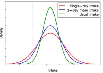
Figure 2. The effect of the within-individual variation on long-term (usual) exposure distributions. This figure is obtained from the National Cancer Institute.
distribution of mean exposures over individuals obtained with OIM will often be too wide in comparison to distributions of ‘true’ long term exposures (compare the green (‘true’ intake) line with the blue line in Figure 2) (Goedhart et al., 2012). For example, the mean exposure assessed over just two days is more variable than the mean exposure assessed over more (up to hundreds) days that constitute a longer period of time. This results in exposures that are about right in the middle of the exposure distribution, but are far too high in the upper tail of the exposure distribution and too low in the lower tail of the exposure distribution).
2.2.2 LogisticNormal-Normal (LNN) model What
Exposure to chemicals via food varies between individuals and between days of the same individual (within individuals). Statistical models that separate these two sources of variation, and subsequently remove the within individual variation from the long-term exposure distribution, have proven useful for the estimation of the long term intake (Dodd et al., 2006; Hoffmann et al., 2002; Slob, 1993). To assess the long-term exposure, variation within individuals is not relevant by definition (the long-term exposure distribution is the variation between individuals, not within individuals), and removal of this source of variation results
therefore in a more accurate estimation of the long-term exposure. LNN is an example of such a statistical model, which is basically very similar to a model published by the National Cancer Institute in the US, known as the NCI model (Tooze et al., 2006). Using LNN, removal of the variation within individuals from the exposure distribution is achieved in the following way. LNN models exposure frequencies and exposure amounts separately, followed by an integration step. By modelling intake frequencies, the model accounts for the fact that for some compounds the intake does not take place every day, but only on a
Page 17 of 41 fraction of the days6 . For the modelling of the positive exposure
amounts, LNN first transforms the positive daily exposure distribution into a more symmetric distribution7. Then a normal distribution8 is fitted to estimate the between-person variation, while removing the within person variation. The resulting between-person normal distribution is then back-transformed and combined with the exposure frequency distribution to obtain the chronic dietary exposure distribution. This is achieved by sampling a large number of times from both the exposure frequency distribution and the back-transformed positive exposure distribution (Monte Carlo integration).
LNN exists in two varieties: with or without assuming and modelling correlation between the exposure frequency and exposure amount. Normally, the variety without correlation is used (sometimes named LNN0), which is the simpler model. MCRA gives the possibility to check how large the correlation is by fitting the full LNN model with
correlation, so that the most optimal variety of the model can be
selected. Furthermore, LNN provides two types of estimates of the long-term exposure distribution: model-based or model-assisted (Goedhart et al., 2012)9. In practice, RIVM normally uses the model-based estimates (see also section 2.2.3).
Using LNN, the long-term exposure can be estimated for specified levels of a covariable (e.g. age) and / or cofactor (sex). As with acute
exposure, also for long-term exposure the most common cofactor / covariable is age. An example of this is the long-term exposure
assessment of dioxins in children aged 2 to 6 years (Boon et al, 2014a) or cadmium in persons aged 2 to 69 years (Sprong & Boon, 2015). Assumptions
LNN assumes that, after a suitable transformation, exposure amounts follow a normal distribution. If this condition is not met at least
approximately, LNN should not be used to assess long-term exposure. As proposed by de Boer et al. (2009), normality can be checked by using the normal quantile–quantile (q–q) plot, a graphical display of observed vs. theoretical residuals. Figure 3 shows an example of a logarithmically transformed positive daily exposure distribution that is acceptable (red line follows the dark line; Figure 3A) and one that is not (Figure 3B). When the fit is not acceptable, LNN should not be used to avoid erroneous long-term exposure estimates. For example, use of LNN in case B of Figure 3 would have resulted in an overestimation of the exposure in the right tail of the exposure distribution.
6 For example, if an individual reports consumption of beer on all person-days which is contaminated with a certain chemical, the model, based on the information on beer consumption in the total food consumption database, estimates the probability that this person will consume beer on all days of a longer period or only a fraction. If in the whole database the number of person-days on which beer consumption is recorded is low, this probability will be estimated to be low.
7 Transformation can be performed with either a logarithmic or power transformation (Goedhart et al., 2012). 8 By fitting a variance components model using the residual maximum likelihood (REML) method.
9 Model-assisted estimates of the long-term exposure distribution are back-transformed values from a shrunken version of the transformed OIM distribution, where the shrinkage factor is based on the variance components estimated using the linear mixed model for amounts at the transformed scale. For individuals with no observed exposure (OIM=0), no model-assisted estimate of long-term exposure can be made and a model-based replacement is used
Page 18 of 41
Figure 3. Histogram together with best fitting normal distribution (left panel) and corresponding q-q plot (right panel). A: acceptable fit; B: unacceptable fit. The lines 1 and 2 correspond with the 97.5th and 99th percentiles of exposure, respectively.
Uncertainties
The main uncertainty of using LNN is that the true long-term distribution may deviate from the assumed normal distribution. This may be
especially true in the tails (both lower and upper) of the distribution. For food safety purposes, the upper tail is most crucial. The 97.5th and 99th percentiles of exposure correspond with theoretical residues of 2 and 2.3 in the q-q plot (Figure 3). In the example, the q-q plot with an
acceptable fit (Figure 3A) shows that these residuals are still reasonably approximated by a normal distribution. In cases where the fit is not acceptable (such as in Figure 3B), very broad normal distributions may be fitted leading to a large overestimation of the upper tail of the
exposure distribution. The acceptance of normality based on the q-q plot may introduce an additional uncertainty, since it is partly based on expert judgement. To reduce the probability of subjectivity, the q-q plot(s) on which the expert judgement is based should always be
discussed among colleague risk assessors. Furthermore, the plots should always be published, for example as an annex to the publication, to allow other experts to judge the appropriateness of the decision. For examples of this, see Boon et al. (2014a,b) and Sprong & Boon (2015).
2.2.3 Model-Then-Add (MTA)
Model-Then-Add (MTA) was developed to address those long-term exposure assessments where the daily positive exposure distribution after transformation is not normally distributed. Non-normality is often
Page 19 of 41
Figure 4. Histogram together with best fitting normal distribution (left panel) and corresponding q-q plot (right panel) for the long-term exposure to patulin. Figure is obtained from de Boer et al. (2009).
due to the contribution of individual foods or food groups to the total exposure that combined result in a multimodal distribution (de Boer et al., 2009). An example of such a distribution was the long-term
exposure to patulin via food due to the consumption of multiple distinct foods, including apple juice, apple sauce and other fruit juices (Figure 4) (de Boer et al., 2009). The same was shown for the exposure
distribution to smoke flavours, which was trimodal due to the intake via three distinct food groups: 1) ‘sausage, frankfurther’ ‘sausage, smoked cooked’ and ‘soup, pea’; 2) ‘bacon’, ‘ham’, ‘herbs’ and ‘sausage,
luncheon meat’, and 3) all other foods (van der Voet et al., 2014). Exposure to patulin and smoke flavours via each of these foods or food groups was shown to be approximately normal (except for the ‘all other foods’ group for smoke flavours).
What
In MTA, a statistical model, such as LNN, or OIM is applied to assess the long-term exposure via subsets of the diet (single foods or food groups), and then the resulting long-term intake distribution per food or food group are added to obtain the overall intake distribution. The advantage of this approach is that the exposure via separate foods or food groups may show a better fit to a normal distribution than the exposure via all foods together.In the add step of MTA, the modelled exposures per food or food group are added to obtain a total exposure intake distribution. There are two approaches for this: distribution-based or individual-based. With the use of the distribution-based approach, exposures per food or food group are independently sampled from the separate exposure distributions and subsequently added. This approach ignores possible correlations between the foods or food groups consumed, and may therefore result in erroneous estimates of the intake if such
dependencies exist. Using the individual-based approach, some aspects of this correlation are included resulting in an improved estimate of the exposure (Goedhart et al., 2012). The distribution-based adding
approach uses the model-based exposure estimates from LNN and the individual-based adding approach the model-assisted exposure
Page 20 of 41
The exposure assessment only benefits from MTA when at least one subset of the diet can be identified for which the exposure can be modelled using a statistical model. If no such food (group) can be identified, MTA has no added value to OIM. Inclusion of covariables or cofactors is not possible in the current version of MTA in MCRA. Assumptions
The major assumption of MTA is that modelling of the exposure via the consumption of subsets of the diet and adding these to obtain the overall exposure results in a better estimation of the exposure than estimating the exposure via all foods together. A first case study into the intake of smoke flavours demonstrated that MTA may result in lower, more refined estimates of long-term exposure in the right tail of the exposure distribution, reflecting high exposure, compared to using either OIM or LNN (van der Voet et al., 2014). Also, simulation studies showed that MTA performs very well and gives good results for the upper percentiles (Goedhart et al., 2012; Slob et al., 2010).
Because MTA uses OIM and LNN to model the exposure per food
(group), the same assumptions apply as described for these two models (section 2.2.1 and 2.2.1, respectively).
Uncertainties
Because MTA is based on OIM and LLN, the same uncertainties apply as described for these two models (section 2.2.1 and 2.2.2, respectively). An additional uncertainty is related to the approach chosen in the add step: with or without taking correlations in food consumption into account. Slob et al. (2010) showed an example where performing the addition step without considering possible correlations in food
consumption performed well, even if correlations in consumptions of foods were present. To test this assumption, the add step of MTA should be performed using both approaches to check if results differ
significantly and if so, if this would have a significant impact on the risk management decision. In case this is true, the cause of the difference should be examined and the best approach should be taken.
2.3 Model input uncertainty
In the previous two sections, we described several probabilistic models to assess the acute and chronic exposure to chemicals via food. The use of these models is subjected to uncertainties. Apart from model
uncertainty, as addressed above per model, the uncertainty is also related to the input data used in these assessments. These input data include food consumption data and concentrations of the relevant chemicals in food. Dependent on the type of chemical additional information may be needed about processing or unit variability. Processing information is needed to adjust chemical concentrations analysed in raw foods (e.g. oranges with peel, lettuce with outer leaves) to those in foods as consumed (e.g. oranges without peel, orange juice). Unit variability is needed to derive concentrations in individual units (e.g. one apple) based on average composite sample (e.g. 15 apples) concentrations (FAO/WHO, 2004). Unit variability is relevant for acute exposure. These inputs are not exhaustive, but are those most
Page 21 of 41 commonly used in exposure assessments. The most common sources of uncertainty related to these input data are:
• Uncertainty due to the size of the food consumption and concentration database
• Biased sampling of food products;
• Concentrations reported below a certain limit value; • Under- or overreporting of the consumption of foods; • Combining of foods consumed to those analysed; • Processing factors;
• Unit variability factors, including number of units in a composite sample and unit weights;
The first uncertainty listed above can be quantified with the use of the bootstrap approach (van Ooijen et al., 2009). With this technique multiple input databases are created from the original input databases with replacement and used to assess the exposure, resulting in a 95% confidence interval10 around the exposure outcomes. See for an example of such outputs Tables 3-1 and 3-2 in Boon et al. (2014a). The more limited the size of the food consumption and concentration data, the broader the confidence interval will be, and subsequently, the larger the uncertainty around the estimated exposure percentiles. Obviously, a broad uncertainty interval is not so serious if the whole interval is far above or far below the relevant health-based guidance value. Estimates in the neighbourhood of such guidance value will benefit most from a reduced uncertainty. The bootstrap approach can also be used to assess the uncertainty due to the size of the food consumption or concentration data, separately. For a more elaborate discussion related to uncertainty about food consumption and concentration data, see section 3.
Apart from bootstrapping, uncertainty can also be quantified using parametric methods. With these methods, the uncertainty in processing factors and concentration data can be modelled, resulting also in
confidence intervals around the exposure estimates. For more details, see van der Voet, et al. (2015) and Kennedy et al. (2015b).
All other sources of uncertainty listed above can either be assessed via sensitivity analyses or qualitatively based on expert judgement as recommended by EFSA (2006). In sensitivity analyses, different values of an input variable are used to study how this affects the exposure outcome. Sensitivity analyses are often used to address the uncertainty related to the concentrations to be assigned to samples reported to contain the chemical at a concentration below a certain limit value, such as the limit of quantification (LOQ), detection (LOD) or reporting
(LOR)11. For an example of this, see Appendix E in Boon et al. (2009). The larger the difference in exposure due to different values of an input variable, the more uncertain the exposure estimate will be. Whether this 10Means e.g. for the P99 that there is a 95% probability that the real P99 of exposure level lies within this interval, and there is therefore a 5% probability that the real P99 is outside this interval: 2.5% probability that the real P99 is higher than the upper level of the confidence limit and 2.5% probability that the real P99 is lower than the lower limit of the confidence interval.
11 Note that in MCRA no distinction is made between LOD, LOQ and LOR. In the literature on performance characteristics of analytical methods important distinctions are made between these concepts in the context of analytical method validation. However, for exposure modelling it is only important that these values have been used as a censoring limit for reporting quantitative outcomes by the data providers.
Page 22 of 41
is acceptable or not will, again, depend on the relation between the exposure estimate and the relevant health-based guidance value, as described above. If not acceptable, additional input data are needed to improve the exposure estimation or it may be decided that an intake assessment is not feasible (see section 3). Examples of a qualitative uncertainty analysis can be found in several exposure publications (Boon et al., 2014a; Boon et al., 2015; Sprong & Boon, 2015).
For a more detailed description of the sources of uncertainty (and others) within exposure assessments, see van Ooijen et al. (2009).
Page 23 of 41
3
Which model to use
In this section, we address which model is most appropriate to use to assess the exposure as close to the true intake as possible. Since there is only one model available to assess the acute exposure for this
purpose and moreover this model makes few assumptions, this section will primarily deal with the models that are available for long-term exposure assessments.
Assessing long-term exposure to chemicals in food is complex, since the reality of the true long-term intake is inherently complex. Many factors determine this long-term intake. To assess this type of exposure, models have been developed to capture this reality in the best way possible. In practice, these models approach reality by making
assumptions about this reality. Therefore, more complex models can be expected to give a better approximation of the true intake, if the
assumptions are valid. But, obviously, complex models have also more opportunities that assumptions are not valid, so their results can also be as far away from the true intake or even further if assumptions are not correct. For a schematic representation of this, without implying
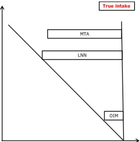
quantitative exactness, see Figure 5. In this sketch the true intake can be found in the upper right corner. Model results can deviate from the true intake in two directions: more to the bottom if the complexity of the real world is not incorporated in the model, and more to the left if model assumptions are not valid.
OIM is a model with few assumptions, and can therefore often be
assumed valid for the estimation of the mean exposure over the survey
Figure 5. Schematic representation of the long-term models in relation to the true intake depending on the validity of the assumptions and their complexity. Complexity and validity cannot be quantified in practice, so this graph is just a qualitative illustration of the concepts.
Increasing validity of assumptions
In cr easi ng com ple xity OIM True intake LNN MTA
Page 24 of 41
Figure 6. Flow diagram of a long-term exposure assessment to adverse substances via food with the aim to assess the exposure as close to the real intake as possible. LNN = Logisticnormal-normal; MTA = Model-Then-Add; OIM = Observed individual means. For more details, see text.
days (section 2.2.1). However, because of this the model is very simple and tail estimates of the exposure distribution will inherently be far from the true long-term intake tail percentiles (Figure 2). LNN is a more complex model, whose output will potentially be closer to the true intake than the OIM estimate of exposure. However, how close to the true intake will depend on the validity of the assumptions (especially the assumption that the exposure amounts follow approximately a normal distribution, section 2.2.2). If the assumptions are not valid, the exposure estimate can be as far from the true intake as the OIM estimate, or maybe even further. MTA is an even more complex model than LNN and can potentially result in exposure estimates that are closer to the true intake than LNN (Figure 5). However, also the use of this model may result in an exposure estimate that is either close or far from the true intake, depending on the validity of the assumptions. Based on the analysis above, LLN is the first model of choice to assess the long-term exposure (Figure 6). This model, if assumptions are valid, results in exposure estimates that are potentially close to the true intake. If however, the assumption of normality is not met
(section 2.2.2) and the exposure estimates show a non-normal
distribution, the more complex MTA model could be used to refine the exposure estimate. If however, no distinct food or food group can be distinguished for which the exposure distribution shows a normal distribution resulting in an acceptable estimation of the long-term exposure, OIM can be selected as a fall-back option (Figure 6). OIM is not based on model assumptions and can therefore always be used to assess the long-term exposure, given the input data allow for this (see below). However, because of its assumptions, it overestimates the intake in the upper tail of the exposure distribution (section 2.2.1), and should therefore only be used if the other two models are not suitable. The model selection should always be motivated in the reporting so that
LNN yes no LNN MTA OK? OK? yes no MTA OIM
Page 25 of 41 it is clear why a certain model has been applied and that this choice can be checked.
Please note that MTA is not recommended as the first choice of model to assess the long-term exposure, although this model potentially results in the optimal exposure estimate (Figure 5). MTA is a more labour
intensive approach and should therefore only be used if the validity of the assumptions of LNN is not met. Furthermore, complex models should only be used if they result in significantly improved estimates of the exposure compared to less complex models. We estimate that this is only the case when the assumptions underlying LNN are not met
(section 2.2.2).
Choice of model in relation to available food consumption and concentration data
In the recommendations of the use of models described above to assess the exposure as close to the real intake as possible, it is assumed that the input data are of good quality and the use of the models is not restricted by this. However, this will often not reflect reality. In practice, the input data may be limited and / or of poor quality. Below we will address this issue by discussing the use of the models in relation to the availability of food consumption and concentration data as the two most important input sources for an exposure assessment to a chemical via food.
For the food consumption, the Dutch food consumption data from the DNFCS are used. These data are based on two days of food recording per person, as recommended by EFSA (2014b). Two days, in
combination with statistical modelling, is the minimum number of days that can be used to estimate the long-term intake distribution of a population (Dodd et al., 2006). According to Bakker et al. (2009), three days would be better. However, it is wiser to use available budgets to obtain food consumption data of more persons on two days than less on three days (Slob et al., 2006). For acute exposure modelling, one food recording day per person would be sufficient to estimate the exposure. The food consumption data from the DNFCS are in general well suitable to model the long-term exposure to chemicals using the different models, except when dealing with those that only occur in very rarely consumed foods (Bakker et al., 2009)12. A recent example of this was the estimation of the long-term intake of nitrite via the consumption of salmon sausage: on only 7 out of 7638 person-days consumption of a relevant food was recorded (Front Office Food and Consumer Product Safety, 2014). In those cases, an estimation of the long-term intake within a population with any of the three models (Figure 5) is not feasible. In the example of salmon sausage, a deterministic approach was therefore used based on a conservative estimate of the daily consumption of salmon sausage in the Netherlands.
12 Simulation studies showed that this is true for foods with a consumption frequency (= fraction of days that the food is consumed) lower than 0.0065 (=0.65%, which corresponds to about 20 and 50 person-days in DNFCS-Young children (Ocké et al., 2008) and DNFCS 2007-2010 (van Rossum et al., 2011), respectively) (Slob, 2006).
Page 26 of 41
In addition to food consumption data, concentration data for the relevant foods need also to be suitable for a reliable exposure
assessment. Two types of concentration data can be distinguished which are commonly used in exposure assessments: monitoring data and concentration data of total diet studies (TDS). Monitoring data are generated by national authorities and are obtained to ensure compliance with maximum limits or indicative values as set in legislation. TDS are mainly performed to assess the long-term exposure to chemicals via food among the general population.
As discussed in Sprong & Boon (2013), the concentration data of chemicals in food should, in the optimal situation, meet at least the following criteria for use in probabilistic exposure assessments, both acute and chronic:
1. Concentrations of relevant chemicals are determined in individual foods as consumed including all possible processing options; 2. The sample size is large enough;
3. Samples are representative for all food products consumed in the Netherlands, which may contain the chemical of interest;
4. True zero concentrations are known for each chemical-food combination;
5. Analyses are performed with analytical methods that analyse at low LOQs;
In practice, the available concentration will very rarely, if ever, meet all these criteria (Sprong & Boon, 2013). For example, monitoring data are often analysed in raw products (e.g. wheat, raw endive, orange with peel) instead of foods consumed and targeted at those most likely to contain the chemical at concentrations above a legal limit value. TDS concentration data are analysed in mixed samples of comparable foods regarding their possible contamination, making their use for acute exposure assessments, without (additional) assumptions about the distribution of the chemical over the individual foods within the mixed sample, not appropriate. For an elaborate description of the
characteristics and (dis)advantages of these two types of concentration data in relation to their use in exposure assessments, see Sprong & Boon (2013).
It is difficult to set criteria for the reliable use of concentration data in a probabilistic exposure assessment. This will depend on a number of factors, of which the most important are the percentile of exposure to be estimated, type of foods included in the assessment, LOQ in relation to the quantified levels, type of assessment (acute vs. chronic), and variability in concentrations within a food:
• The percentile of exposure will determine the minimal number of exposure estimates that are needed to describe the exposure distribution within a population. In exposure assessments, this number is dependent on a combination of consumption and concentration values of many foods. A standard result, based on a non-parametric method, is that at least 59 and 298 exposure estimates are needed to estimate the P95 and P99 of an
Page 27 of 41 have been used by EFSA to calculate P95 and P99 food
consumption statistics from the Comprehensive13. • The type of food analysed is relevant in relation to its
contribution to the overall exposure to the chemical. If limited data or poor quality data are available for a food that does not contribute significantly to the exposure (e.g. rarely eaten foods, foods with very low chemical concentrations), they may still be used in the exposure assessment. If it however concerns a major contributor, it should be examined if the quality of the data can be improved (see below).
• The LOQ of the analytical method may result in a conclusion that the exposure estimate is very uncertain if the number of samples with an analysed level below the LOQ is large and / or the
quantified levels are close to the LOQ. In those cases, the
exposure estimates may largely depend on the levels assigned to the non-quantified samples. An example of this is the use of screening methods with high LORs to analyse multiple chemicals (Boon et al., 2009).
• The type of assessment may also be an important factor. In an acute exposure assessment, the whole range of possible
concentrations per food that people may encounter in real life needs to be considered, whereas for a chronic exposure assessment a mean concentration per food suffices. This
difference may result in other conclusions about the suitability of the concentration data available.
• When the variability in concentration values within a food is low, the sample size needed to obtain representative concentrations of that food will be smaller than when the variation is large. Sample size is an important aspect of concentration data. However, a clear indication of an adequate (= minimum) number of concentrations needed to obtain a reliable exposure estimate is hard (if not impossible) to give. In the literature, no clear guidance regarding sample size is available. For example, the EFSA guidance on probabilistic modelling only states that a minimum of two samples is needed to model the concentration per food parametrically via a lognormal distribution (EFSA, 2012). This number is however based on the minimal data requirements to fit a lognormal distribution and has no relation to data quality. In TDS, a sample size of 12 per food (group) is recommended (Ruprich, 2013). However, this number may not always be sufficient to obtain reliable concentrations per food (group) (Sprong et al., 2015). Sample size should therefore be addressed per chemical and food analysed. When the sample size is judged to be too small, there are a number of options to increase it. These options are listed here in random order:
1. Obtaining additional data from the literature; 2. Grouping of foods with comparable characteristics; 3. Parametric modelling of concentration data.
4. Additional analytical measurement in foods 13 www.efsa.europa.eu/en/datexfoodcdb/datexfooddb.htm
Page 28 of 41
Which of these options (one or more) should be chosen depends on the chemical. For example, if concentrations in certain foods for a specific chemical are not expected to vary between European countries, concentration data as published by EFSA may be used to increase sample size or to fill data gaps. This was for example done in a study into the exposure to lead in the Netherlands, in which (reliable) Dutch data on lead in wheat, rice and eggs were not available and therefore obtained from EFSA (Boon et al., 2012). Grouping of foods may be relevant when foods can be identified that are expected to contain comparable levels of the chemical of interest. This was for example done to assess the dietary exposure to lead in five European countries (Boon et al., 2014b). Parametric modelling may be useful when the observed concentrations per food are not expected to represent the whole range of possible concentrations to which a population may be exposed. Using parametric models based on the observed data, concentrations above, between and below the observed values per food can be modelled (van der Voet et al, 2015). This approach is recommended in the acute pessimistic model run of the EFSA guidance on probabilistic modelling and the refined chronic exposure assessment (EFSA, 2012). As stated above, to use this option at least two quantifiable concentrations per analysed food are needed and the use of a lognormal distribution is recommended (EFSA, 2012). In a recent exposure assessment of methylmercury (MeHg) intake in children ages 2 to 15 years in the Netherlands this approach was used to describe the concentration data of MeHg in different foods (Front Office Food and Consumer Product Safety, 2015). Another option is to generate additional concentrations in foods for which no (reliable) data are available and which are deemed important for the exposure estimate. Examples of this are analyses of cadmium in peanut butter (Sprong & Boon, 2015), and flame retardants in fruit and vegetables (Boon et al., in prep.). In practice, this last option may not be used often because of the costs involved. Obtaining additional data from the literature or from additional measurements in foods can also be used to improve the quality of concentration data that do not cover all relevant foods. The use of concentration data known to be targeted to foods within a food group expected to be highly contaminated (e.g. when visible from the outside of the food in case of mycotoxins or obtained from a suspect country in the case of pesticide residues) in an exposure assessment should be avoided as much as possible. If this results in low sampling sizes or missing data for certain foods, the options described above can be used to address this.
Based on the analysis above, the minimum requirements of the concentration data used in an exposure assessment are:
• Coverage, possibly via mapping to foods consumed, of all relevant foods that may contain the chemical,
• It is known how the data are obtained (monitoring, targeted sampling, TDS, etc.),
• Analysed with a validated analytical method. • Sample size should be adequate
It is impossible to state these requirements in a general quantitative form. Rather, they should be checked case by case, and they must be considered in the context of the risk assessment question. For example,
Page 29 of 41 the sample size for a certain food may be very low, but this is less important if the contributions of other foods are the main risk drivers or if exposure estimates are far below toxicologically relevant levels even when considering sampling uncertainty. Dependent on the chemical addressed, additional minimum requirements may also be needed before the concentration data are suitable for use in an exposure assessment.
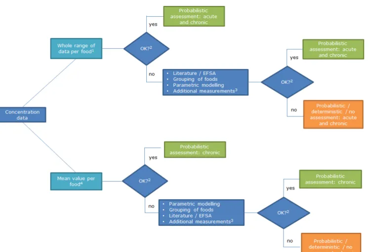
If the quality of the concentration data cannot be improved as indicated above or only partly, it has to be discussed whether the exposure models (section 2) are nevertheless the best way forward to estimate the intake as close to the true intake as possible. This discussion requires a comparison with alternative options, such as the use of a deterministic approach to obtain an indication of the possible exposure. A conclusion may also be that no reliable exposure assessment can be performed. Figure 7 shows an overview of the different steps regarding the evaluation of the available concentration data for use in exposure assessments.
Overall, probabilistic exposure assessments will always be performed in situations of limitations regarding concentration data which can either be major or minor. These limitations can be reduced, if relevant, using the above options, but will never be completely removed. A probabilistic exposure assessment should therefore always include an uncertainty analysis regarding the concentration data used (as well as other input variables), as recommended by EFSA (2006, 2012) (section 2.3). If the data are of too poor quality, but a probabilistic exposure assessment is performed despite this, it should always be argued why the exposure assessment is performed (e.g. obtain insight in possible health risks or foods contributing potentially largely to the exposure as input for generation of concentration data), and the limitations of the exposure output should be addressed. Examples of such assessments are the preliminary assessment of the exposure to 3-monochloropropane-1,2-diol (3-MCPD) via food (EFSA, 2013), and the one to mycotoxins in children aged 2 to 6 in the Netherlands (Boon et al., 2009). In those cases, conclusions regarding the exposure estimates and possible health risks should mirror these uncertainties. For example, in the case of the exposure assessment to mycotoxins, it was recognised that the
concentration data were (partly) targeted (Boon et al., 2009). Exposures below the relevant health-based guidance values were therefore judged to indicate negligible health risk. However, for exposures above the guidance values no conclusion was possible about possible health risks due to the very likely overestimation of the exposure. In those cases, it was concluded that ‘Determination of health risk is not feasible’ (Boon et al., 2009).
Page 30 of 41
Figure 7. Flow diagram of concentration data to be used in probabilistic exposure assessments. 1Monitoring programs, and total diet studies (TDS) using assumptions regarding distribution of concentration data over individual foods within TDS sample;2 Refersto minimum requirements met (p 28); 3 See text for details; 4 Monitoring programs and TDS.
Page 31 of 41
4
Additional model functionalities
In this document, we have focussed on the most commonly used functionalities available within MCRA to assess the acute and chronic exposure assessment.
The MCRA software is continuously being updated, including the implementation of user wishes to improve its use, but also new
functionalities, like the implementation of MTA in 2013 (van der Voet et al, 2014). Some of the other functionalities / options are described shortly below.
4.1 Optimistic and pessimistic exposure assessment
In 2012, the EFSA guidance on the use of the probabilistic methodology for modelling dietary exposure to pesticide residues was released (EFSA, 2012). In this guidance, two model runs are proposed, an optimistic and a pessimistic model run for both acute and chronic exposure
assessments. In the optimistic model run, the major uncertainties of the assessments are treated using assumptions that are expected to result in lower estimates of exposure, whereas in the pessimistic model run these uncertainties are treated in such a way that it is expected to result in overestimates of exposure. This provides the risk manager a range for the true exposure and a tool for decision making. When in the optimistic model run the exposure estimate exceeds the health-based guidance value14, the true exposure will be higher and risk reduction measures should be taken. In case the pessimistic model run results is below the health-based guidance value, the risk manager can be confident that the true exposure will be even lower and no risk reduction measures are needed. Any other outcome needs further investigation, e.g. by refining the exposure assessment.
In MCRA, the settings needed to assess the optimistic and pessimistic exposure to chemicals have been implemented. Via the calculation options ‘EFSA Guidance Optimistic’ and ‘EFSA Guidance Pessimistic’ the user can very easily select all the correct settings belonging to the two calculation scenarios. These options are available for the assessment of the exposure to both single and multiple (see section 4.2) chemicals. This implementation was performed within the EU project ACROPOLIS (Boon et al, 2015; van der Voet et al., 2015).
4.2 Cumulative exposure assessment
For some chemicals, sharing the same toxicological effects, it may be relevant to assess the exposure simultaneously instead of chemical by chemical. These types of assessments can be performed with MCRA using the relative potency approach as described in EFSA (2012). Examples of such assessment are the exposure to groups of pesticides, including organophosphates and carbamates (Boon et al., 2008, 2009), and pesticides of the triazole group (Boon et al., 2015). The acute and 14 For example, the acceptable or tolerable daily intake (ADI, TDI) for chronic exposure and the acute reference dose (ARfD) for acute exposure.
Page 32 of 41
chronic models can be used to assess cumulative exposure. This implementation was also performed within the EU project ACROPOLIS (van der Voet et al., 2015). The H2020 project EuroMix will extend upon the model developed in this EU project.
4.3 Aggregate exposure assessment
Within MCRA there is the possibility to assess the exposure to chemicals via dietary and non-dietary routes, such as air or skin, which was also implemented as part of the EU project ACROPOLIS (Kennedy et al., 2015a). In this implementation, the dietary exposure is calculated as described in section 2. The exposure via non-dietary routes needs to calculated outside MCRA and then uploaded onto the program. MCRA will then combine the exposure via food with that of the non-dietary sources to arrive at a total exposure. The linking of exposure via both sources (dietary and non-dietary) can be performed by matching individuals based on their characteristics, such as age and sex, or randomly.
This implementation of aggregate exposure in MCRA is a first prototype of how such an assessment can be performed using probabilistic
techniques (van Klaveren et al., 2015). The H2020 project EuroMix will add on to these fundaments.
Page 34 of 41
5
Conclusion
This document describes the probabilistic models available to assess the acute and chronic exposure to chemicals via food as close to the true intake as possible in MCRA and which have been used in the last two years by the RIVM in scientific papers, (letter) reports and in
assessments of the Front Office Food and Consumer Product Safety. When the aim is to estimate the exposure as close to the true intake as possible, probabilistic models should be used. We recommend the use of LNN, followed by MTA if needed (Figure 6), for a long-term exposure assessment. If the use of MTA is also not feasible due to violation of its underlying assumptions, OIM can be used, realising that it
overestimates the intake in the upper tail of the exposure distribution. The model selection should always be motivated in the reporting so that it is clear why a certain model has been applied and that this choice can be checked. For an acute exposure assessment, only one basic model is available to assess the exposure as close to the true intake as possible, the probabilistic Monte Carlo approach.
If these models are however used as part of a risk assessment (start simple and conservative, and only proceed to more advanced, refined approaches if a health risk cannot be ruled out), the choice of models may be different than described in this document. In that case,
deterministic models will often be chosen in the first tier (e.g. PRIMo for the acute or chronic exposure to pesticide residues via food (EFSA, 2007)), and the first probabilistic model of choice to assess long-term exposure may be OIM instead of LNN. The reason for this is that these options are less labour intensive.
Use of all models addressed in this document is data dependent. It should therefore always be examined if the data allow the use of the models. For food consumption data, it is assessed that the data of the Dutch national food consumption surveys mostly allow their use, except for very rarely consumed foods. For concentration data this is less clear, and will depend on a case-by-case judgement of the concentration data available and foods involved. Furthermore, for both acute and chronic models, many decisions regarding submodelling aspects will determine the ‘precision’ of the exposure estimate. For example, how to match foods-as-eaten to those analysed, and whether or not to model
processing factors, unit variability, and concentrations below LOQ, LOD and / or LOR.
Overall, the models described in the document represent the current state of art regarding exposure modelling to adverse chemicals via food, and allow in many cases for the most realistic exposure estimates currently possible.
Page 36 of 41
Acknowledgements
The authors would like to thank Corinne Sprong and Jan Dirk te
Biesebeek of the RIVM, and Jacqueline Castenmiller, Rob Theelen, Dirk van Aken and Marca Schrap of the NVWA-BuRO for their valuable comments on earlier versions of this document.
Page 38 of 41
References
Bakker MI, Fransen HP, Ocké MC, Slob W (2009). Evaluation of the Dutch National Food Consumption Survey with respect to dietary exposure assessment of chemical substances. RIVM report 320128001. National Institute for Public Health and the Environment (RIVM),
Bilthoven. Available online: www.rivm.nl.
Boon PE, Bakker MI, van Klaveren JD, van Rossum CTM (2009). Risk assessment of the dietary exposure to contaminants and pesticide residues in young children in the Netherlands. RIVM report 350070002 National Institute for Public Health and the Environment (RIVM), Bilthoven. Available online: www.rivm.nl.
Boon PE, te Biesebeek JD, de Wit L, van Donkersgoed G (2014a). Dietary exposure to dioxins in the Netherlands. RIVM letter report 2014-0001. National Institute for Public Health and the Environment (RIVM), Bilthoven. Available online: www.rivm.nl.
Boon PE, te Biesebeek JD, van Donkersgoed G, van Leeuwen S, Hoogenboom LAP, Zeilmaker MJ (in prep.). Dietary exposure to
polybrominated diphenyl ethers in the Netherlands. National Institute for Public Health and the Environment (RIVM), Bilthoven.
Boon PE, te Biesebeek JD, Sioen I, Huybrechts I, Moschandreas J,
Ruprich J, Turrini A, Azpiri M, Busk L, Christensen T, Kersting M, Lafay L, Liukkonen K-H, Papoutsou S, Serra-Majem L, Traczyk I, De Henauw S, van Klaveren JD (2012). Long-term dietary exposure to lead in young European children: comparing a pan-European approach with a national exposure assessment. Food Additives and Contaminants: Part A 29: 1701-1715.
Boon PE, van der Voet H., Ruprich J, Turrini A, Sand S, van Klaveren JD (2014b). Computational tool for usual intake modelling workable at the European level. Food and Chemical Toxicology 74: 279-288.
Boon PE, van der Voet H, van Raaij MTM, van Klaveren JD (2008). Cumulative risk assessment of the exposure to organophosphorus and carbamate insecticides in the Dutch diet. Food and Chemical Toxicology 46: 3090-3098.
Boon PE, van Donkersgoed G, Christodoulou D, Crépet A, D’Addezio L, Desvignes V, Ericsson B-G, Galimberti F, Ioannou-Kakouri E, Jensen BH, Rehurkova I, Rety J, Ruprich J, Sand S, Stephenson C, Strömberg A, Turrini A, van der Voet H, Ziegler P, Hamey P, van Klaveren JD (2015). Cumulative dietary exposure to a selected group of pesticides of the triazole group in different European countries according to the EFSA guidance on probabilistic modelling. Food and Chemical Toxicology 79: 13-31.
de Boer W, Goedhart PW, Hart A, Kennedy MC, Kruisselbrink J, Owen H, Roelofs W, van der Voet H (2015). MCRA 8.1 a web-based program for Monte Carlo Risk Assessment. Reference Manual. September 1, 2015. Biometris, Wageningen UR, National Institute for Public Health and the Environment (RIVM) and Food and Environmmental Research Agency (Fera), Wageningen, Bilthoven, The Netherlands and York, UK.
Page 39 of 41 de Boer WJ, van der Voet H, Bokkers BGH, Bakker MI, Boon PE (2009). Comparison of two models for the estimation of usual intake addressing zero consumptions and non-normality. Food Additives and
Contaminants: Part A 26: 1433-1449.
Dodd KW, Guenther PM, Freedman LS, Subar AF, Kipnis V, Midthune D, Tooze JA, Krebs-Smith SM (2006). Statistical methods for estimating usual intake of nutrients and foods: a review of the theory. Journal of the American Dietetic Association 106: 1640-1650.
EFSA (2006). Opinion of the Scientific Committee related to
uncertainties in dietary exposure assessment. The EFSA Journal 438: 1-54. Available online: www.efsa.europa.eu.
EFSA (2007). Pesticide Residues Intake Model for assessment of acute and chronic consumer exposure to pesticide residues-rev.2. Available online: www.efsa.europa.eu.
EFSA (2011). Use of the EFSA Comprehensive European Food Consumption Database in Exposure Assessment. EFSA Journal 9(3):2097, 34 pp. Available online: www.efsa.europa.eu.
EFSA (2012). Guidance on the Use of Probabilistic Methodology for Modelling Dietary Exposure to Pesticide Residues. EFSA Journal 10(10):2839, 95 pp. Available online: www.efsa.europa.eu.
EFSA (2013). Analysis of occurrence of 3-monochloropropane-1,2-diol (3-MCPD) in food in Europe in the years 2009-2011 and preliminary exposure assessment. EFSA Journal 11(9):3381, 45 pp. Available online: www.efsa.europa.eu.
EFSA (2014a). Food Additives Intake Model (FAIM): comments received from stakeholders and EFSA’s views. EFSA supporting publication 2014:EN-566. 25 pp. Available online: www.efsa.europa.eu.
EFSA (2014b).Guidance on the EU Menu methodology.EFSA Journal 12(12):3944, 77 pp. Available online: www.efsa.eu.europa.
EFSA (2015a). Refined exposure assessment for Quinoline Yellow (E 104). EFSA Journal 13(3):4070, 33 pp. Available online:
www.efsa.europa.eu.
EFSA (2015b). Scientific Opinion on acrylamide in food. EFSA Panel on Contaminants in the Food Chain (CONTAM). EFSA Journal 13(6):4104, 321 pp. Available online: www.efsa.europa.eu.
FAO/WHO (2004). Pesticide residues in food - 2003. Report of the Joint Meeting of the FAO Panel of Experts on Pesticide Residues in Food and the Environment and the WHO Core Assessment Group. FAO Plant Production and Protection Paper, 176. Geneva. Available online:
www.fao.org/fileadmin/templates/agphome/documents/Pests_Pesticides
/JMPR/Reports_1991-2006/Report_2003.pdf.
Front Office Food and Consumer Product Safety (2014). Assessment of nitrite in salmon sausage (in Dutch). National Institute for Public Health and the Environment (RIVM), Bilthoven.