Effects of bail-ins on European banks

EFFECTS

OF

BAIL-INS

ON

EUROPEAN BANKS

Aantal woorden / Word count: 20.984

Tom Remue

Studentennummer / student number : 01510379

Promotor / supervisor: Prof. Dr. Rudi Vander Vennet

Masterproef voorgedragen tot het bekomen van de graad van:

Master’s Dissertation submitted to obtain the degree of:

Master in Business Engineering: Finance

Academiejaar / Academic year: 2019-2020

I

VERTROUWELIJKHEIDSCLAUSULE

PERMISSION Ondergetekende verklaart dat de inhoud van deze masterproef mag geraadpleegd en/of gereproduceerd worden, mits bronvermelding.

II Preface

This dissertation was written with the goal of achieving my master in business engineering : finance.

I want to thank prof. Dr. Vander Vennet and Nicolas Soenen for letting me work on this interesting topic and helping me along the way. I also want to thank Dan, Jan and Steven for proofreading and my family for supporting me during my studies.

III

Preamble for master’s dissertations impacted by the corona measures

The research was originally planned to Investigate the effects of a bail-in on European banks using an event study approach. Because the needed data and information was all available online I didn’t experience much trouble due to the coronavirus. The meetings were not done in person anymore, but the online tool (Microsoft teams) worked efficiently and didn’t hinder much.

“ This preamble is drawn up in consultation between the student and the supervisor and is approved by both”.

IV

Content

2.3 ARGUMENTS FOR BAIL-IN ... 8

2.4 POSSIBLE PROBLEMS ... 9

3.EMPIRICAL METHOD AND DATA ... 11

3.1 EMPIRICAL METHOD ... 11

3.2 DATA ... 14

4.EXPECTATIONS ... 18

5.EVENT OVERVIEW... 20

6.SELECTED CASES AND RESULTS ... 25

6.1 AMAGERBANKEN ... 25

6.2 SNS REAAL ... 30

6.3 BANK OF CYPRUS AND LAIKI ... 36

6.4 UK CO-OPERATIVE BANK ... 42

6.5 REGULATION EVENTS ... 46

6.6 BANCO ESPIRITO SANTO ... 56

6.7 ANDELSKASSEN JAK SLAGELSE ... 62

6.8 FOUR ITALIAN BANKS ... 66

6.9 NOVO BANCO ... 70

6.10 BANCO POPULAR ESPANOL ... 74

6.11 VENETO BANCA AND BANCA POPOLARE DI VICENZA ... 78

7.CONCLUSION ... 82

8.SAMPLE OVERVIEW ... 84 9.REFERENCE LIST ... VII 10. APPENDIX ... XII

V

List of figures

Figure 1: Bail-in hierarchy ... 4

Figure 2: Example of a bail-in ... 7

Figure 3: Scale-Location example ... 13

Figure 4: Average total return index of sample ... 16

Figure 5:Average CDS spreads of sample ... 17

Figure 6: Cumulative total returns pre-regulation ... 21

Figure 7: Cumulative CDS spreads pre-regulation ... 21

Figure 8: Cumulative total returns of regulation events ... 22

Figure 9: Cumulative CDS spreads of regulation events ... 22

Figure 10: Cumulative total returns between regulation and implementation ... 23

Figure 11:Cumulative CDS spreads between regulation and implementation ... 23

Figure 12: Cumulative total returns post-implementation ... 24

VI

List of tables

Table 1: Amagerbanken[-5,5], total return index ... 27

Table 2:Amagerbanken[-5,5], daily total return index, t=’07-02-2011’ ... 28

Table 3: Amagerbanken [-5,5], CDS spreads, daily dummy variables ... 29

Table 4:Amagerbanken [-5,5], CDS spreads, one event dummy ... 30

Table 5:SNS Reaal [-5,5], total return index ... 32

Table 6: SNS Reaal [-5,5], Total return index, daily dummy variable ... 33

Table 7:SNS Reaal [-5,5], CDS spreads ... 34

Table 8:SNS Reaal [-5,5], Daily CDS spreads, constant return model ... 35

Table 9:Cyprus [-5,5], Total return index ... 38

Table 10:Cyprus [-5,5], total return index, daily dummy variables ... 39

Table 11:Cyprus [-5,5], Daily CDS spreads, daily dummy variables ... 40

Table 12:Cyprus [-5,5], Daily CDS spreads, constant return model ... 41

Table 13:UK Co-operative [-5,5], Total return index, daily dummy variables ... 43

Table 14:UK Co-operative [-5,5], CDS spreads, daily dummy variables ... 44

Table 15:UK [-5,5], CDS spreads ... 45

Table 16: Proposal [-5,5], Total return index ... 47

Table 17: Proposal [-5,5], Daily total return index, daily dummy variables ... 48

Table 18: Proposal [-5,5], CDS spreads, constant return model, daily dummy variables ... 49

Table 19: Proposal [-5,5], CDS spreads, Market model, daily dummy variables ... 50

Table 20: Parliament agreement[-5,5], total return index ... 52

Table 21: Parliament agreement[-5,5], total return index, daily dummy variables... 53

Table 22: Parliament agreement[-5,5], CDS spreads constant return model, daily dummy variables . 54 Table 23: Parliament [-5,5], CDS market model, daily dummy variables ... 55

Table 24: Espirito [-5,5], Total return index ... 57

Table 25: Espirito [-5,5], Total return index, Daily dummy variables ... 58

Table 26:Espirito [0,3], Total return index ... 59

Table 27:Espirito [-5,5], CDS spreads, daily dummy variables ... 60

Table 28 : Espirito [-2,2], CDS spreads ... 61

Table 29:Andelskassen [-5,5], Total return index... 63

Table 30: Andelskassen [-5,5], Total return index, daily dummy variables ... 64

Table 31:Andelskassen [-5,5], CDS spreads, Daily dummy variables ... 65

Table 32:Italy [-5,5] , Total return index ... 67

Table 33:Italy [-5,5] , Total return index, daily dummy variables ... 68

Table 34:Italy [-5,5] , Daily CDS spreads, daily dummy variables ... 69

Table 35: Novo Banco [-10,10], Total return index ... 71

Table 36: Novo Banco [-5,5], total return index, daily dummy variables... 72

Table 37: Novo Banco [-5,5], CDS spreads, daily dummy variables ... 73

Table 38: Banco Popular [-5,5], Total return index ... 75

Table 39: Banco Popular [-5,5], Total return index, daily dummy variables ... 76

Table 40: Banco Popular [-5,5], CDS spreads, daily dummy variables ... 77

Table 41: Veneto [-5,5], Total return index ... 79

Table 42: Veneto [-5,5], Daily Total return index, daily dummy variables ... 80

1

1.INTRODUCTION

After the 2008 financial crisis followed by the sovereign debt crisis, there were many complaints about the bail-out procedure. After the collapse of Lehman brothers, European governments understood they needed to save their systemic banks in order to prevent a full collapse of the financial system and consequently the economy. An action of which some countries still carry consequences today, the level of debt of some of the European countries is extremely high compared to their GDP, which decreases fiscal capacity and makes the bail-out procedure increasingly harder to execute.

Adding to that, taxpayers had to pay for the mistakes of the financial institution’s management and greed which caused a severe moral hazard problem, breaking a key principle of the free market economy being that owners and creditors are supposed to bear the losses of a failed venture. Another problem was that the subordinated creditors were also being bailed out by taxpayers in the same way as the senior creditors, which caused creditor inertia (Gleeson, 2012).

This has led to the introduction of the EU Bank Recovery and Resolution Directive (BRRD) and the Single Resolution Board (SRB), followed by the Bail-in tool and other resolution functions on January 1, 2016. Although, even before the implementation of those, multiple European countries already adopted the bail-in approach.

In this dissertation I will research the effects of a bail-in event on the total return indices and the CDS spreads of other European banks using an event study approach. I expect, due to a higher risk premium and reduced bail-out expectations, CDS spreads to rise and stock returns to go down after the announcement of a bail-in. I choose most events that used the bail-in tool from several European countries like Denmark, Spain, Portugal,… and also two events concerning the announcement of the European agreement on the implementation of the requirement of using bail-ins.

There exists a wide policy-oriented literature on the use of bail-ins ( for example, Gleeson, 2012 ; Avgouleas and Goodhart, 2016; Avgouleas and Goodhart, 2015). (Guliana, 2017) also finds that positive indications of commitment to bail-in increased the difference in yield between unsecured (i.e., bail-inable) and secured (i.e., non-bailinable) bonds. Interestingly, events indicating a decreased commitment towards the bail-in, reduce the yield spread between unsecured and secured bonds. My dissertation adds to the small literature of empirical effects of bail-ins and to the discussion on the credibility of the BRRD and the banking union. It gives us an answer to the question whether the use of a bail-in does have an impact on the market view on the riskiness of banks which could indirectly have a negative impact on banks’ funding costs (CDS is an indication of riskiness of the

2

banks which translates into higher funding costs) and hereby potentially putting more pressure on the profit margins of the European banks. Secondly it also gives us an indication which events had a bigger impact than others and was the impact limited to other domestic banks or more

internationally? Lastly, it also analyses bail-in events after the implementation of the bail-in tool together with the SRB which has not been done before to my knowledge.

I will first discuss the bail-in tool with a short explanation of the framework, a theoretical example of how the bail-in should work, arguments for the use of bail-in and possible problems. In the third part I will discuss the data and the empirical method, followed by prior expectations in part four. Next I will give an event overview followed by the selected cases in detail together with the results in part six, and the conclusion of the research will follow in part seven.

2.BAIL-IN

2.1 FRAMEWORK

The bail-in tool is a procedure to be used by the resolution authorities and allows them to write down and convert the claims of creditors into equity. This implicitly means that the creditors will have to take the losses instead of the taxpayers as before during the “bail-outs”. The writing down is done by following a hierarchy of creditors determined by the SRM regulation. Creditors that belong to the same hierarchy should be treated equally, however within the same class of creditors exclusions are possible.

Not all liabilities are to be written down, certain liabilities are excluded from the scope of the bail-in tool. For example deposit amounts that fall under the deposit guarantee scheme (DGS) are also excluded, but any amount higher than the DGS could be bailed-in. Secured liabilities are also partially ‘at risk’ in a way that the difference in value between the liability and the collateral securing it can also be potentially bailed-in.

Some examples of liabilities that haven been excluded from the bail-in tool are:

– covered deposits, i.e. deposits up to the amount covered by a deposit guarantee scheme (DGS)

– employee remuneration or benefits

– liabilities to tax and social security authorities that are preferred by law

For a full overview I refer to ‘the Handbook of Basel III Capital: Enhancing Bank Capital in Practice’ by Juan Ramirez (2017).

3

In specific conditions certain liabilities can be partially or fully excluded from the bail-in by the resolution authorities, even if this means that creditors within the same class are not going to be treated equally. Some examples of these exceptional conditions are :

– it is not possible to bail-in the liability within a reasonable timeframe (this could potentially apply to derivatives liabilities, which can be very difficult to value in a short space of time); or

– the exclusion is necessary and proportionate to achieve continuity of critical functions and core business lines.

An important principle to hold in account with this is the NCWOL (No creditor worse off than under liquidation principle). This provision cannot be broken when applying the resolution. Because the resolution authorities can exclude liabilities form the bail-in, it can also increase the level of write-down or conversion of the other liabilities to compensate for this. Following the NCWOL principle, this can only be done if these creditors absorbing the losses would not be worse off than they would have under normal insolvency proceedings. Further valuations will have to be made to determine whether this is the case. The bail-in tool also needs to follow a concrete order of creditors to be bailed-in first. The first ones to bear the losses however must always be the shareholders. The prescribed order for creditors is aligned with the procedure in normal insolvency proceedings, that way the NCWOL provision won’t be as easily violated. However the question remains when the bailed-in creditors actually are worse off than under normal insolvency proceedings, by whom should they be compensated and in what form? A suggestion could be shares.

In the case when the non-absorbed losses still needed to be absorbed due to exclusion of liabilities can’t be passed on to the other creditors, the resolution financing arrangement can support by making a contribution to cover the unabsorbed losses. They are for example able to purchase shares or capital instruments of the institution so that the bank in resolution will be able to restore itself and be recapitalized sufficiently. However this is conditional to a prior 8% of bail-in that needs to be executed first, before the resolution fund or government support can be used. Thus meaning that the institution under resolution has already absorbed losses of at least 8% of its total liabilities including own funds. This 8% has to be measured at the moment it is decided that the institution is at the point of failing or likely to fail (FOLTF), thus when the resolution is announced. Also, the funding provided by the resolution fund can’t exceed 5 % of total liabilities including own funds.

4 Bail-In hierarchy

During a Bail-in action, as mentioned before, the existing shareholders are to be hit first. The shares will be cancelled or transferred to the bailed-in creditors. This will thus lead to a severe dilution of the existing shareholders or for them to be totally wiped out depending on the required amount of bail-in.

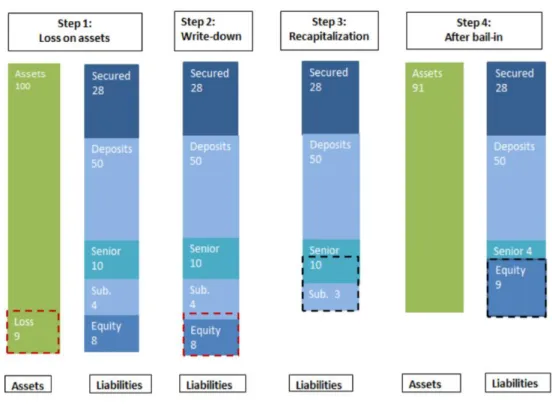
Usually, the majority of the liabilities being bailed-in will be the unsecured debt instruments. This can be done after the exercise of rights embedded in the terms of the instrument where there is a certain condition that can trigger conversion(contingent convertible bonds for example) or after decision of the resolution authority. Figure 1 gives an overview of the total hierarchy that needs to be followed during the bail-in.

Figure 1: Bail-in hierarchy

source: European commission

Necessary conditions

Three main conditions for resolution should be met in order for the bail-In tool to be used. First, there can’t be any prospect that any alternative private sector measures would prevent the failure within a reasonable timeframe. Secondly, the resolution action is necessary and in the public interest and lastly, the financial institution has to be at the point of failing-or-likely-to-fail (FLTF).

5

This determination is made by the supervisor or the resolution authority, and does not have a quantitative threshold.

MREL and TLAC

In order to avoid that the financial institutions would restructure their liabilities in a way that their borrowings could not be touched and thus give their creditors immunity from the bail-in tool, the BRRD has introduced the Minimum Requirement for Own Funds and Eligible Liabilities (MREL). This expresses a minimum level of loss-absorbing liabilities that need to be held by the financial

institution relative to its own funds and total liabilities. It sets up a sufficient loss absorbing and recapitalization capacity in resolution. These loss-absorbing liabilities will mostly consist out of own funds (capital) and inable liabilities. However, it is good to mention that not all of these bail-inable liabilities count towards the institution’s MREL. This is because there is uncertainty as to how feasible it is for some of these liabilities to be bailed-in in an actual resolution scenario.

The BRRD requires the MREL to be based on the bank-specific features, including its size (systemic importance), business model, funding model and risk profile. The targets are set by EU resolution authorities together with the prudential supervisors and can also be influenced by the desire to limit contagion effects and the level of possible negative impact on non-professional creditors.

The MREL has a similar aim to the Total loss Absorbing capacity (TLAC) standard that was developed by the Financial Stability Board (FSB). This being that G-SIBs(Globally systemic important banks) need to have the capacity to recapitalize via a bail-in procedure. However some differences are important, one being that the TLAC was designed specifically for global systemically important banks (G-SIBs) at an international level. Another apparent difference is that the TLAC standard also includes measures to strongly dis-incentivize for financial institutions to hold liabilities that are likely to be bailed in at the point of resolution of another institution. Hereby thus limiting contagion effects that could present themselves during a bail-in procedure. G-SIBs must deduct these holdings that are exposed to other external TLAC liabilities issued by other G-SIBs from their own TLAC. In the MREL

requirement there is not a similar deduction included. However the national resolution authorities can be instructed to limit the extent to which financial institutions possess another institution’s liabilities that are eligible for bail-in.

6 Level of recapitalization

The bail-in tool ultimately is applied to recapitalize the financial institution that is failing or likely to fail (FLTF) to a level that this institution can continue carrying out its normal activities for which it is authorized and to comply with the regulations that are set for the institution to be authorized. On top of that it is extremely important for the institution that market confidence is sufficiently restored.

There is no specific level of recapitalization that needs to be achieved, it is like the FLTF assessment very much more of a qualitative assessment made by the resolution authorities complying with the draft Regulatory Technical Standards(RTS) made by the European Banking Authority (EBA). In short these RTS aim for the institution to have a level of MREL that mainly satisfies the capital

requirements applicable, can match the average level of capitalization of a peer group in order to regain market confidence and be able to absorb losses sufficiently.

In order to successfully reorganize, the institution’s management or other authority has to prepare a business reorganization plan they have to submit to the resolution authority within one month of the bail-in. With this plan it has to be clear that after implementation the long term viability of the institution is restored. Within a month after the submission the resolution authority must assess and agree to this, or has to give additional instructions which they find necessary.

7

2.2 EXAMPLE

Figure 2: Example of a bail-in

source: European central bank

With the framework and concept explained, I will now introduce a short example using figure 1 to show how the working principle of the bail-in tool.

To trigger the procedure, the bank in the example incurred a loss of 9 percent on its total assets. To absorb these losses we look at the liabilities side, we can see that in this example the institution’s liabilities consist of 8% equity that will be totally wiped out following the bail-in hierarchy

(shareholders are the first line of defense). Next, subordinated debt will also be written down until all losses are absorbed. In this example there is sufficient subordinated debt to absorb the remaining losses so not all of it will be used (only 25% of the subordinated debt). During the third phase, still following the hierarchy, the liabilities will be converted into equity until a sufficient recapitalization level is achieved. In our example the total amount of remaining subordinated debt will not be sufficient, so also senior unsecured debt will be bailed-in.

After this conversion has happened the balance sheet will look like the one in step 4. The financial institution is recapitalized and will meet its capital requirements again. Of course this is an example of how it would work ideally, possible problems that might come with the execution of the bail-in will be discussed later.

8

2.3 ARGUMENTS FOR BAIL-IN

A key element of the bail-in procedure is trying to enhance the market discipline of the financial institutions. By implementing the potential that the costs of the failure of a financial institution would fall on creditors, these who own liabilities of a financial institution which are eligible for bail-in have a stronger motive to monitor the institution’s risk of failure. Considering the risk premium attached to the bail-in nature of the debt instruments, banks could offset the increased funding costs (“due to this bail-in risk premium”) by increasing/improving their credit profile. (Lewrick et al, 2019) find evidence that this “bail-in risk premium” indeed is being adopted by the investors. Adding to this, they find that investors in riskier banks get rewarded by a larger premium, however the

investors’ monitoring eases with more comfortable market-wide conditions and this is being used as a good time to issue bail-in instruments by the financial institutions. (Giuliana, 2017) also finds that bail-in events weakly increase investors' incentives to incorporate a bank's risk into the prices of its securities, consistent with an improvement of market discipline.

Another mechanism for enhancing market discipline might be that, as the potential costs of bank failure would fall on creditors, in addition to shareholders, such creditors should become more alert about the levels of leverage the bank carries, limiting one of the most likely causes of bank failures and the governance costs associated with excessive leverage. Normally, shareholders have every incentive to build leverage to maximize their return on equity (Avgouleas and Cullen, 2015).

So overall you could say that the funding costs of the bank will rise taking this risk-premium into account and the requirement of bail-inable liabilities. However opposite to this you could argue that in return the bank should have a safer structure, due to the higher market discipline, and this could then actually lower the funding costs.

Also, once the bail-in and resolution is completed the assets remaining should be less risky compared to before the bail-in as you have written of the bad assets, this hints to the fact that the capital requirements should actually be equal or lower than before bail-in.

One of the biggest advantages of course is the removal of the moral hazard problem that was apparent during bail-outs of financial institutions. Taxpayers, in principle, should not have to cover anymore for the mistakes of the bank’s management. You could argue whether it is better to let a few take a lot of loss than a lot taking a relatively small loss and why the investors in pension funds, other institutions or individual savers are better placed to absorb the losses. These investors do often not really have the expertise to act as effective bank monitors. However the reasoning there is that

9

they have made a clear decision the purchase the claim on the bank as opposed to the taxpayer (unless the instruments have been mis sold like in a specific case in Italy that is discussed later on.)

Another major advantage is that, in principle, the financial institution should be able to continue its operations as a going concern. Execution of the bail-in, if done right, can be very fast with minimum disturbance of the customers and destruction of value.

Furthermore, as mentioned in the framework it would need less of capital injected from the national authorities and is very much needed to improve the fiscal capacity of some European countries.

Finally, as the regulatory requirements focus (MREL) on G-SIBS, there could be an incentive to split banks or reduce the footprint. Hereby thus dealing with the too-big-to-fail problem that is still quite apparent.

2.4 POSSIBLE PROBLEMS

The bail-in procedure has to be timed well, if it is done too early, this can lead to multiple rounds of bail-in which is far from ideal. Opposite of this might be that if the timing is too late creditors, especially other institutionals who monitor very closely, could be able to flee from the institution which would put the institution in further problems. Potentially leading to a public bank run if confidence is lost as we have seen in the past and putting a lot of pressure on the liquidity. There is still no theoretical model of the criteria for intervention of resolution authorities (quantification of loss absorption buffer; estimation of potential extreme losses, choice of intervention

thresholds)(Goodhart and Segoviano, 2015). This can cause frictions and loopholes, for example during the liquidation of Veneto Banca and Banca popolare di Vicenza there was a lot of criticism on this issue.

This flight of creditors can also be a major problem at other financial institutions, when an institution is in problems due to non-specific firm problems and the bail-in is triggered it might alarm creditors of other institutions. This can create difficulties and contagion effects, especially in worse economic conditions. It is not uncommon in Europe that a banks’ debt is held by another bank which could then be bailed-in also, spreading contagion effects further and increasing systemic risk. (Avgouleas and Goodhart, 2016) mention that in times where there is a systemic problem, bail-ins can trigger a bank funder panic both ex ante and ex post. The BRRD acknowledges this problem and therefore Injection of public funds (including temporary public ownership under Article 58 BRRD) is allowed in any case only in ‘the very extraordinary situation of a systemic crisis’ subject to approval under the

10

Union state aid framework (BRRD). Obviously this problem should be smallest when the failure of the financial institution is caused by very firm-specific risks, for example because of bank fraud during good conditions.

Adding to this, in Italy for example one third of bondholders were other domestic banks and there was an historically high level of debt held by households (World bank group, 2016). Meaning there is a lack of internationalisation of the Italian debt market as well. This could further spill over effects and could potentially be dangerous in the case of a larger bail-in. This is one of the reasons that the resolution of ‘Monte dei Paschi di Siena’ in Italy did not follow the BRRD, because they were very concerned that pensioners for instance would lose all their savings in banks’ bonds. Hereby hurting the credibility of the BRRD and the SRB. This indicates a major issue of the bail-in, for example when a pension fund is bailed-in and faces big losses, many(f.i. pensioners) will be impacted indirectly. This is not specific to Italy.

Also we have to keep in mind that, after the bail-in, management will probably be replaced and there are other perspectives being introduced. New accountants, appointed by the resolution agency, could view the scenario way more negative than the ones before because they were incentivized to take a more positive view on the valuation. This transition could thus lead to a big drop in published accounting valuations which would mean another hit to the institution.

Another potential problem could be a difference in treatment of the domestic creditors and the foreign creditors. Resolution authorities might be biased as towards which creditors to bail in, as already happened before and was even organized like this for Icelandic banks in the past. We also saw this argument come in to play during the bail-in of 5 selected bonds of Novo Banco (a case I will discuss later). To tackle this problem, the BRRD disallows discrimination between creditors based on their nationality or other characteristics.

Next, with bail-in regimes in place, there is a serious risk of pro-cyclicality which is not wanted in the banking system, hence the countercyclicality buffers. By bailing-in the banks become weaker and it will get more expensive for them to get funding also. Thus, a shift away from bail-out towards bail-in is likely to reinforce pro-cyclicality. The ECB has been cautious about bailing-in bank bondholders for such reasons in the past (Andrew G. et al, 2016).

One more weakness of a bail-in as a bank restructuring tool is that it does not provide any new cash. Thus in order to survive the firm must not only be creditworthy, but credibly creditworthy to at least its central bank, and soon after to the market as a whole.

11

It is therefore likely that bail-in will require statutory backing in order to convince counterparties to continue dealing with it post-reconstruction.(Gleeson, 2012)

3.EMPIRICAL METHOD AND DATA

3.1 EMPIRICAL METHOD

To investigate whether the bail-in event has an impact on the stock returns and CDS spreads I will make use of the event study regression method as suggested by Pynönnen (2005). An event study is a great method to measure the impact of a specific event on the value of a firm’s equity or debt securities(Mackinlay, 1997). It estimates the value of the selected variable during an event by using data prior to the event and then compares these estimated values with the actual values during the event.

First, I choose an estimation window length of 120 days to limit possible estimation errors and I will use event windows with varying lengths to investigate possible anticipation effects. The daily returns from the total return indices or first differences in CDS spreads calculated from the collected data will be regressed on the daily returns or CDS spread difference of the market variable, creating hereby a single index market model with the coefficient 𝛽 as the market beta. To handle the potential

problem of contemporaneous correlation due to having the same event windows for the firms, which might lead to bias in the standard error estimates, I use an equally weighted portfolio suggested by Pynönnen(2005), Jaffe(1974) and Brown and Warner(1985). Brown and Warner (1985) also found that the market model was robust in the presence of cross correlations by simulating abnormal returns using actual return data for randomly selected samples.

Besides this I also create dummy variables which will have a one value on a day which is part of the event window and a zero value when not. This causes the coefficients of the dummy variables to capture abnormal effects during the event windows. If an event window happens to take place during an estimation period for another event we leave this out of that estimation period and we include prior trading days to still have an exact 120 days in the final estimation window.

The regression then goes as follows for the daily returns of the total return indices:

𝑟𝑝,𝑡 = 𝛼𝑝+ 𝛽𝑝𝑟𝑚,𝑡+ ∑ 𝛾𝑝,𝑛 𝑡2 𝑛=𝑡1

𝐷𝑡,𝑛+ 𝜇𝑝,𝑡

𝑟𝑝,𝑡 will equal the average of the daily returns of all the banks included in the sample (equally

weighted portfolio) for the event on day t. 𝑟𝑚,𝑛 equals the daily returns of the market index, in this

12

𝐷𝑡,𝑛 are dummy variables that equal to one on event day n = t and zero otherwise, n = t1, t1+1,…,t2.

Meaning that the coefficient 𝛾𝑝,𝑛 should capture any abnormal differences that occurred during the

event.

For the CDS spreads I use two different methods to run the event study regression.

The first method will use a market model just like the regression used for the total return indices:

∆𝐶𝐷𝑆𝑝,𝑡 = 𝛼𝑝+ 𝛽𝑝∆𝐶𝐷𝑆𝑚,𝑡+ ∑ 𝛾𝑝,𝑛𝐷𝑡,𝑛 𝑡2

𝑛=𝑡1

+ 𝜇𝑝,𝑡

The regression will work identical to the first one, With ∆𝐶𝐷𝑆𝑝,𝑡 denoting the average of the daily

difference in CDS spreads of the banks included in the sample on day t. ∆𝐶𝐷𝑆𝑚,𝑡 represents the daily

difference of the DS EUROPE BANKS 5Y CDS INDEX on day t.

the second method is a constant return model:

∆𝐶𝐷𝑆𝑝,𝑡 = 𝛼𝑝+ ∑ 𝛾𝑝,𝑛𝐷𝑡,𝑛 𝑡2

𝑛=𝑡1

+ 𝜇𝑝,𝑡

Where 𝛼𝑝 should equal the mean of the first differences of the CDS spreads and the coefficient of

the dummy variables should capture the abnormal effects (same mechanism as with the market model). I use these two models firstly to compare results and because I suspect that the DS EUROPE BANKS 5Y CDS INDEX potentially could also have an impact from the event and hereby mitigate the abnormal effects. Another reason I use two methods is because for some regressions the market factor did not seem to be significant, if this is the case the model actually falls back to a similar constant return model statistically but to make sure I then used the second model separately. (Mackinlay, 1997) also finds similar conclusions using these two methods but finds a larger standard error and some loss of precision. After running both, the results are qualitatively largely the same in my research as well. If the difference is remarkable both regressions will be given.

The null hypothesis in these event study regressions is that the actual return on the event day or during the event window does not statistically significantly differ from the estimated return. This means that if the dummy variable for example has a p-value of <0.01, we can reject the null

hypothesis with 99% certainty and assume that the actual return does significantly differ (positively or negatively) from the estimated return.

13

I will always start by evaluating the impact on the full sample of European banks in our data, then I will check for the contagion effects in specific countries. For example for the bail-in of Banco popular Espanol SA I will also check for the contagion effects on only Spanish banks and also on only other Southern countries like Italy and Greece. To be able to do this I split up the full sample of banks in to different subsamples( ‘Mediterranean’, ‘Scandinavian’,…) visible in Table 1.

However, if for example I investigate the Banco popular bail-in event I want to see the contagion effects on Spanish banks and other ‘Mediterranean’ banks separately so for this case I take the Spanish banks out of this subsample. The same I will do for the Amagerbanken event, taking the Danish banks separately and leaving them outside the ‘Scandinavian’ sample.

After running the regressions I also check for potential heteroskedasticity problems that could occur due to patterns in the variance of the residuals and hereby potentially causing biased results. I check for this in two ways. I check this graphically by looking at the scale-location plot. If this plot gives a straight line with no specific pattern in the observations the model does not have a

heteroskedasticity problem. Hereby an example:

Figure 3: Scale-Location example

To verify a second time I use the Breush-Pagan test developed by T.Breusch and R.Pagan in 1979 implemented in Rstudio. Only if this test has a p-value is lower 0.05 we can reject the null hypothesis of homoskedasticity at the 95% confidence level. None of the events seem to suffer from

14

3.2 DATA

I selected specific cases that made use of the bail-in tool with respect to the size of the institution that was resolved, the amount that was bailed-in, which level of creditors were hit and the importance that it might have on other institutions. Meaning not every single case with a bail-in is included in the study, but those that are included were in my opinion the most indicative, important events and are also well spread over time. To this day, not a single financial institution has been fully resolved by using the bail-in tool alone like in the given example(not in combination with sale of business for example). Besides these I also include events that happened around the implementation and regulation of the bail-in, these should give us a great indication how the market reacted on the introduction and announcement of the bail-in tool as a requirement.

The data I use are the total return indices and the CDS spreads of different banks from across Europe obtained from Datastream and markIt (full overview in section 8. Sample overview). For the market total returns index I use the total return indices of the EuroStoxx50 and I also use the Stoxx global 1800 for comparison for the events I have access to it. The EuroStoxx50 is an index that is designed to represent the 50 largest companies in the Eurozone by market capitalization. The index holds stocks from 11 Eurozone countries and is managed and licensed by STOXX Limited, which is owned by Deutsche Börse AG. It is also reviewed annually to evaluate the index components in September.

As of January 8, 2020, the top ten components in the Euro STOXX50 Index included the following:

• Total SA • SAP SE

• ASML Holding NV

• LVMH Moet Hennessy Louis Vuitton SE • Linde PLC • Sanofi SA • Siemens AG • Allianz SE • Airbus SE • Unilever NV

The Stoxx global 1800 is more of a broad representation of the world’s most developed countries, including 600 European countries, 600 American and 600 Asian/pacific companies.

15

I mainly use the Euro Stoxx 50 because they seem to be a stronger estimator for the European banks and I lack the data of the Stoxx global 1800 for some events. However I still do compare the results to see if there are no big differences due to the European banks possibly also affecting the Euro Stoxx 50 more as they make up about 7% of the index (at the present) and hereby possibly mitigating effects. After comparison, the results were qualitatively largely the same and only the Euro Stoxx 50 is used in the results tables.

I choose to work with the total return indices because it assumes that any cash distributions, such as dividends for example, are reinvested back into the stock. This way we look at both the yield of the stock and the capital gains creating a more accurate view on the total performance. For example when a stock has a capital gain of 8% over the year and also an annual yield of 3%, the total return will show a growth of 11% in total for the year. If the same stock had a drop of 3% in share price, the total return would be 0%. Comparing to price returns, which do not take into account cash

distributions, it makes a significant difference in return.

We will then convert these total return indices into daily returns (DR) in percent by subtracting the index of the day before from the day now and dividing this by the index of the day before.

𝐷𝑅𝑡 =

𝑅_{𝑡 –} 𝑅_𝑡−1 𝑅𝑡−1 ∗ 100

16

Figure 4: Average total return index of sample

Figure 4 shows an overview of how the total return index has evolved for our sample of banks compared to the market factor (Euro stoxx 50). We can see that since the financial crisis the banks’ returns index has gone down by a lot and hasn’t been able to fully recover yet to pre-crisis levels. The market however did go up a lot percentage wise since the crisis over these years. At the end of the graph we can also notice the impact of the coronavirus already putting further pressure on the banks.

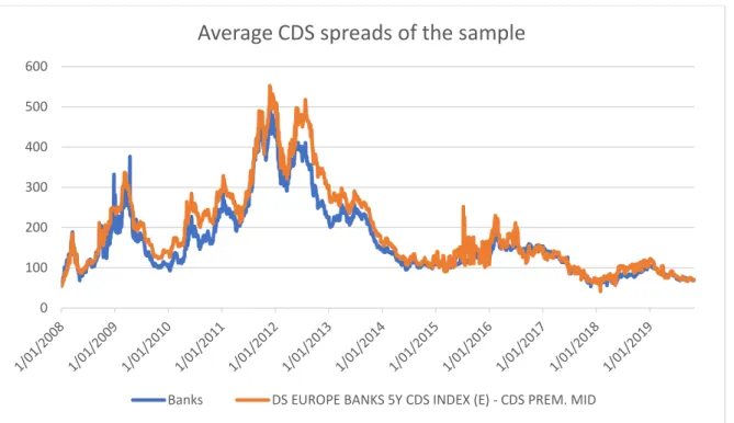
The second variable we want to perform the event study on are the credit default swap spreads of the financial institutions. A credit default swap (CDS) is a derivative instrument you can buy which will pay you if a certain company defaults. The "spread" of a CDS is the annual amount the protection buyer must pay the protection seller over the length of the contract, expressed as a percentage of the notional amount. So this translates to, the higher the spread you need to pay, the higher the probability of default. Furthermore, Bouveret (2009) finds that CDS spreads serve to estimate default probabilities expected by markets and are thus a leading indicator of fears over the solvency of borrowers. So this is a good variable to be used to measure market confidence and indirectly also the funding costs. The market factor used for the regression here is the DS EUROPE BANKS 5Y CDS INDEX. 0 1000 2000 3000 4000 5000 6000 7000

Average total return index of sample

17 ∆𝐶𝐷𝑆𝑡 =

𝐶𝐷𝑆𝑡 – 𝐶𝐷𝑆𝑡−1

𝐶𝐷𝑆𝑡−1 ∗ 100

Figure 5:Average CDS spreads of sample

Looking at the evolution of the CDS spreads in Figure 5 we can notice that, like the total returns, the CDS spreads evolved in a negative way after the financial crisis and peaked around the sovereign debt crisis in 2012. However, opposed to the total returns, the CDS spreads were able to recover to normal levels recently. We can also notice that the banks are very alike with our market factor, that is why I also include the constant return model, the DS EUROPE BANKS 5Y CDS INDEX might absorb too much of the effects.

For selecting the event date used for the event window I choose to pick the announcement dates that the troubled bank was officially going to be bailed-in. This should be the day that it gets out to the public and where the effects should happen. As it is difficult to determine possible sentiment or expectations the event window will be started 5 days before the event date and end 5 days after. In this way I will be able to notice possible anticipations on the event or leaked information. I was able to find the event dates online through news articles from qualitative financial newspapers (for example ‘The financial times’) , other academic research (f.i. Schäfer et al., 2016) and press announcements from the resolution authorities like the SRB.

0 100 200 300 400 500 600

Average CDS spreads of the sample

18

4.EXPECTATIONS

Before running the event regressions I expect to see a drop in the stock returns and an increase in the CDS spreads. The use of a bail-in means that shareholders and other creditors take a loss, when shareholders of other banks see this happen this should lead to a drop in confidence but also leads to a higher risk level. These effects could translate to lower share prices and a drop in the total returns of European banks, but also to a higher risk of defaulting thus higher CDS spreads.

Another reasoning could be that when there is a use of the bail-in method, the expectations of a bailout at other banks could decrease. Thus implying a direct increase in the probability of default and the feeling that the shareholders and other creditors won’t get saved like they maybe expected. This, again, leading to higher risks and ultimately to a drop in returns and a rise in CDS spreads. These higher CDS spreads or higher ‘riskiness’ can ultimately also lead to higher costs of funding and thus reduces profits also (this could be potentially compensated by banks increasing their loan rates).

Furthermore, I expect the reactions to be different to each specific bail-in case, as we haven’t seen any very similar resolutions with a bail-in yet. Reactions should be higher according to the level of creditors that were bailed in, because here is where the most difference is being made comparing to a bail-out and the strongest signal is sent. For example I expect effects to be higher if senior debt and uninsured deposits also get bailed-in.

I also expect these effects to be most apparent at banks located in the same country as were the bail-in takes place. This because they fall under the same national regulations, but also because they have more similar market conditions and it will be more covered in the news influencing local investors.

For announcements or decisions relating to the regulations of the SRB and the bail-in tool I expect participating countries of the Eurozone of course to be more affected than non-participating. It will be interesting to see if these non-participating countries do get affected at all. Furthermore, I expect G-SIBs to be affected more as well in their CDS spreads because as previously mentioned, they have higher capital and MREL requirements than other banks. I also expect the ‘Mediterranean’ sample specifically to experience a higher impact because during this period these banks were most affected by the sovereign-debt crisis resulting to be seen by the public as most vulnerable and unstable banks, like Greece for example. Opposite to this I expect the ‘Scandinavian’ banks to be least affected, they have been seen as more healthy banks situated in a financially better environment. The asset quality between the two groups has been divided also, with the ‘Southern’ banks having much worse asset quality (Fitch: EU Bank North/South Asset Quality Divide Persists).

19

Because of this worse position they are in it is logical that they are seen as more risky and been perceived to be more likely to make use of bail-in because of lower fiscal capacity to bail-out in the first place. Besides that Denmark for example already had a similar regulation in place with “Bank Package III” and also Sweden and Denmark have their own currency and are not part of the banking union at the time.

20

5.EVENT OVERVIEW

Event Date Country

Amagerbanken 07.02.2011 Denmark

SNS Reaal 1.02.2013 Netherlands

Bank of Cyprus and Laiki 18.03.2013 Cyprus

25.03.2013

UK Co-Operative bank 17.06.2013 UK

Proposal 20.03.2014 EU

EU Parliament back SRM 15.04.2014

Banco Espirito Santo 04.08.2014 Portugal

Andelskassen 05.10.2015 Denmark

Banca Marche, Cassa di Risparmio di Ferrara, Banca Etruria

e CariChieti 23.11.2015 Italy

Novo Banco 29.12.2015 Portugal

Banco popular Espanol 06.06.2017 Spain

Veneto Banca, Banca popolare di Vicenza 23.06.2017 Italy

Here we have a complete overview of all the selected events together with the event date and the country where the resolution took place. We can split these events up into 4 different groups. The first 5 events can be seen as the pre-regulatory events which happened before the agreement on the requirement of the bail-in tool. Then we have two events regarding to the dates where the

agreement on the bail-in happened. After that we have 4 events which happened between the decision on the bail-in tool and the implementation of the regulations (January 1, 2016). The last two events are then events that happened after the implementation. To start I will show some graphs from these four event groups over an event window of [-5,5], thus starting 5 days before the event and ending 5 days after.

The following graphs of these four groups will give us a general idea of what to expect results wise during the event windows. The graphs represent the average percentual change of the banks during the event windows and also of the market index that is used in our regressions.

Going over these graphs we can immediately see some differences in the reactions, especially in the CDS spreads there seems to be quite a difference between the pre-regulation events and the regulation events. Where the pre-regulation events seem to be following our expectations, the post-regulation events’ CDS spreads seem to react quite differently which is interesting to see. In figure 6 for example on the event day t we see the total returns of banks dropping while the market went up by around the same amount.

21

However it is important to say that we can’t really make any conclusions on these graphs because we need to first filter out the dependence on the market movements also which can play a big role in these evolutions. Also these graphs are averaged over the full sample of banks, thus we can’t see reactions for specific groups. In the next part I will go into detail on each case.

Pre-regulation

Figure 6: Cumulative total returns pre-regulation

Figure 7: Cumulative CDS spreads pre-regulation

-3,5 -3 -2,5 -2 -1,5 -1 -0,5 0 0,5 t-5 t-4 t-3 t-2 t-1 t t+1 t+2 t+3 t+4 t+5

Cumulative total returns (%) [-5,5]

Banks Euro stoxx 50

0 2 4 6 8 10 12 t-5 t-4 t-3 t-2 t-1 t t+1 t+2 t+3 t+4 t+5

Cumulative CDS spreads (%) [-5,5]

22 Regulation events

Figure 8: Cumulative total returns of regulation events

Figure 9: Cumulative CDS spreads of regulation events

-2,5 -2 -1,5 -1 -0,5 0 0,5 1 1,5 2 t-5 t-4 t-3 t-2 t-1 t t+1 t+2 t+3 t+4 t+5

Cumulative total returns (%) [-5,5]

Banks Euro stoxx 50

-5 -4 -3 -2 -1 0 1 2 t-5 t-4 t-3 t-2 t-1 t t+1 t+2 t+3 t+4 t+5

Cumulative CDS spreads (%) [-5,5]

23 Between regulation decision and implementation date

Figure 10: Cumulative total returns between regulation and implementation

Figure 11:Cumulative CDS spreads between regulation and implementation

-1,5 -1 -0,5 0 0,5 1 1,5 t-5 t-4 t-3 t-2 t-1 t t+1 t+2 t+3 t+4 t+5

Cumulative total returns (%) [-5,5]

Banks Euro stoxx 50

-4 -2 0 2 4 6 8 10 12 14 t-5 t-4 t-3 t-2 t-1 t t+1 t+2 t+3 t+4 t+5

Cumulative CDS spreads (%) [-5,5]

24 Post-implementation

Figure 12: Cumulative total returns post-implementation

Figure 13:Cumulative CDS spreads post-implementation

-1,5 -1 -0,5 0 0,5 1 t-5 t-4 t-3 t-2 t-1 t t+1 t+2 t+3 t+4 t+5

Cumulative total returns (%) [-5,5]

Banks Euro stoxx 50

-16 -14 -12 -10 -8 -6 -4 -2 0 2 4 t-5 t-4 t-3 t-2 t-1 t t+1 t+2 t+3 t+4 t+5

Cumulative CDS spreads (%) [-5,5]

25

6.SELECTED CASES AND RESULTS

6.1 AMAGERBANKEN

The very first case using the bail-in tool happened in Denmark, which had the “Bank Package III” (“Bank Package III saw the general state guarantee removed and creditors expected to bear the risk of the failure of a financial institution as an incentive to reinvigorate the market mechanism and the pricing of risk”, World bank Group) setup in their national resolution procedure at the time and this prescribed the use of bail-in. Aiming for the same goals as the SRB now does. Amagerbanken was a small retail bank in Copenhagen with total assets amounting to around 4.5 billion euro so the amount was not very high. However senior debt was also hit during the procedure, which gave of a strong signal.Hence, depositors and other unsecured creditors of this distressed bank could not be sure to receive full coverage of their claims.

I quote Ivan Zubo of BNP Paribas at the time : “At a Friday night Board meeting on 4 February, the Directors of the bank determined that the additional write-downs in Q4 2010 of DKK3.14bn implied the equity capital of the bank as of 1 January 2011 would be proforma negative DKK0.7bn. The bank subsequently informed the Danish FSA that it did not meet the solvency requirements. The FSA responded with an order for the solvency requirements to be met by 7pm on 6 February. As no acquirer or investor could be found in such a short period of time (i.e. over the weekend), the supervisory board of the bank elected for the bank to be wound down under the new Danish legislation approved in June 2010 and in force since 1 October 2010. Hence, all the assets and some liabilities have been transferred to a new company, Amagerbanken af 2011 A/S, which is wholly owned by Financial Stabilitet A/S (‘Financial Stability’), the government’s bank resolution fund. Equity and subordinated debt are to stay at the bankrupt entity and hence most likely be wiped out.”

After the resolution, it was estimated that holders of senior debt and unsecured depositors would face a haircut of 41 percent. This was a first time in Europe so the Amagerbanken resolution is a very important case to include into our research.

In the aftermath of the resolution several Danish banks were complaining about a higher cost of funding due to the risk that creditors could be bailed-in. Moody’s also downgraded credit ratings of six Danish banks which has an impact on the cost of funding. Other European countries were looking at the situation closely because they were thinking about adopting the bail-in rules in their

26

effect surely on other Danish banks and possibly on other countries as well. However we have to keep in mind that Denmark does not belong to the Eurozone and this could definitely limit contagion effects.

Results

The Amagerbanken bail-in was a very local event because of the bank and the bail-in amount being relatively small. Next to that, the bail-in regulation was specific to the national regulation of Denmark at the time and this is what we find back in the results here. We can see a statistically significant drop in daily returns for the Danish banks in our sample on the announcement date until three days after the announcement. Three days after the event we can even see a statistically significant drop for our full sample of banks, which is due to not only the Danish banks but also mostly due to the

‘Mediterranean’ banks which are included here. This is not totally against the expectations because the banks of these countries were probably in the most vulnerable situation with the European sovereign debt crisis in mind.

For the CDS spreads we only have one Danish bank in sample(Danske bank, which is a very big and stable bank) so it is hard to draw conclusions here although we can say that we don’t see any negative abnormal reactions for Danske. For the other banks there seems to be no abnormal reactions in the CDS spreads.

Thus, although being a relatively small event we do find some contagion effects for the daily returns, especially at Danish banks as expected.

27

Table 1: Amagerbanken[-5,5], total return index

======================================================================= Dependent variable: --- Banks Scandinavian Danish Mediterranean (1) (2) (3) (4) --- `EURO STOXX 50` 0.510*** 0.609*** 0.153*** 1.028*** (0.028) (0.060) (0.046) (0.064) EVENT 0.022 -0.181 -0.513*** -0.005 (0.108) (0.233) (0.179) (0.251) Constant -0.042 0.057 0.053 -0.202*** (0.031) (0.068) (0.052) (0.073) --- Observations 131 131 131 131 R2 0.729 0.449 0.128 0.667 Adjusted R2 0.725 0.440 0.114 0.662 Residual Std. Error (df = 128)0.342 0.740 0.568 0.798 F Statistic (df = 2; 128) 172.113*** 52.128*** 9.385*** 128.198*** ======================================================================= Note: *p<0.1; **p<0.05; ***p<0.01

28

Table 2:Amagerbanken[-5,5], daily total return index, t=’07-02-2011’

======================================================================= Dependent variable: --- Banks Scandinavian Danish Mediterranean (1) (2) (3) (4) --- `EURO STOXX 50` 0.509*** 0.610*** 0.156*** 1.024*** (0.028) (0.061) (0.046) (0.065) t-5 -0.303 0.382 -0.537 0.425 (0.338) (0.745) (0.562) (0.802) t-4 0.215 -0.045 -0.349 0.704 (0.342) (0.752) (0.568) (0.810) t-3 0.407 -1.007 -0.198 0.203 (0.338) (0.745) (0.562) (0.802) t-2 0.423 0.052 -0.006 0.466 (0.339) (0.746) (0.563) (0.803) t-1 0.007 -1.439* 0.252 -0.456 (0.338) (0.745) (0.562) (0.802) t -0.051 -0.082 -1.697*** -0.340 (0.339) (0.747) (0.563) (0.804) t+1 -0.088 0.058 -0.184 -0.177 (0.338) (0.745) (0.562) (0.802) t+2 -0.017 -0.117 -1.529*** 0.711 (0.338) (0.745) (0.562) (0.802) t+3 -0.942*** -0.712 -1.157** -2.040** (0.338) (0.745) (0.562) (0.802) t+4 0.365 1.311* -0.274 0.491 (0.338) (0.745) (0.562) (0.802) t+5 0.232 -0.392 0.031 -0.033 (0.338) (0.745) (0.562) (0.802) Constant -0.042 0.057 0.053 -0.202*** (0.031) (0.068) (0.051) (0.073) --- Observations 131 131 131 131 R2 0.757 0.490 0.218 0.692 Adjusted R2 0.733 0.439 0.139 0.661 Residual Std. Error (df = 118)0.337 0.742 0.560 0.798 F Statistic (df = 12; 118) 30.677*** 9.461*** 2.747*** 22.130*** ======================================================================= Note: *p<0.1; **p<0.05; ***p<0.01

29

Table 3: Amagerbanken [-5,5], CDS spreads, daily dummy variables

======================================================================= Dependent variable: --- Banks Scandinavian Danish Mediterranean (1) (2) (3) (4) --- `EUROPE BANKS 5Y CDS INDEX`0.894*** 0.568*** 0.504*** 0.970*** (0.074) (0.062) (0.084) (0.085) t-5 -1.417 0.909 -0.757 -1.729 (1.558) (1.310) (1.774) (1.792) t-4 -0.844 -0.914 -5.822*** -2.272 (1.569) (1.319) (1.787) (1.805) t-3 -0.315 -0.018 -0.194 -0.727 (1.554) (1.307) (1.770) (1.788) t-2 0.990 0.047 -0.013 -0.983 (1.553) (1.306) (1.769) (1.786) t-1 -1.476 0.137 -0.190 -1.776 (1.554) (1.307) (1.770) (1.788) t 0.433 0.653 0.660 0.210 (1.553) (1.306) (1.769) (1.787) t+1 1.096 0.229 -0.600 1.237 (1.554) (1.307) (1.770) (1.788) t+2 0.575 0.386 1.589 -0.084 (1.558) (1.310) (1.775) (1.793) t+3 0.655 0.063 -1.184 -0.130 (1.553) (1.306) (1.769) (1.787) t+4 -0.667 -0.283 1.198 -0.418 (1.553) (1.306) (1.769) (1.787) t+5 1.484 0.621 -1.336 1.788 (1.553) (1.306) (1.769) (1.786) Constant 0.089 -0.009 0.397** 0.217 (0.144) (0.121) (0.164) (0.166) --- Observations 131 131 131 131 R2 0.577 0.431 0.324 0.557 Adjusted R2 0.534 0.373 0.255 0.512 Residual Std. Error (df = 118)1.546 1.300 1.761 1.779 F Statistic (df = 12; 118)13.435*** 7.442*** 4.711*** 12.387*** ======================================================================= Note: *p<0.1; **p<0.05; ***p<0.01

30

Table 4:Amagerbanken [-5,5], CDS spreads, one event dummy

======================================================================= Dependent variable: --- Banks Scandinavian Danish Mediterranean (1) (2) (3) (4) --- `EUROPE BANKS 5Y CDS INDEX`0.903*** 0.570*** 0.529*** 0.985*** (0.071) (0.059) (0.083) (0.082) EVENT 0.054 0.168 -0.584 -0.433 (0.480) (0.398) (0.564) (0.553) Constant 0.085 -0.010 0.387** 0.211 (0.141) (0.117) (0.166) (0.162) --- Observations 131 131 131 131 R2 0.561 0.424 0.253 0.539 Adjusted R2 0.554 0.415 0.242 0.532 Residual Std. Error (df = 128)1.512 1.256 1.777 1.743 F Statistic (df = 2; 128) 81.899*** 47.058*** 21.725*** 74.853*** ======================================================================= Note: *p<0.1; **p<0.05; ***p<0.01 6.2 SNS REAAL

SNS Reaal, consisting out of SNS bank and the insurance company Reaal N.V., fell short EUR 1.9 billion of its capital requirements in February 2013. Consequently the Dutch national bank (DNB) ordered an immediate redress. A month before this, share prices already tumbled due to negative press reports and deposits were being withdrawn. SNS did not meet the deadline of the DNB, and the group got nationalized. As the BRRD was not in place during that time, many other options were considered first but proved to be unable. SNS Reaal qualified as a systemic important financial institution and its bankruptcy would have had serious consequences for the stability of the financial system in the Netherlands. The Bail-in tool was partially used in the final resolution, shareholders and subordinated debt holders were being fully bailed-in and resulted in losses of approximately EUR 240 million and EUR 1.67 billion respectively. As this resolution approach was also unprecedented in the Netherlands at this level many legal proceedings followed, this could point ant the unexpectedness of the bail-in approach, something we should take into account for our results. As the bail-in of shareholders and subordinated debt holders alone was not enough there was also an injection of

31

capital of EUR 3.7 billion by the ministry of finance, restructuring and a levy by the treasury of a ‘one-off tax’ on the banking sector amounting EUR 1 billion. As a result the group was nationalized and the board members were replaced. Although the creditors that were included were limited (senior debt was saved) it was the first bail-in that involved a considerable amount of money and also a first systemically important bank using the bail-in.

The financial institution was also considerably big in the Netherlands which made it an important event. It took place when there were already talks of reforming the European banking regulations. The Finance Minister in the Netherlands at the time was Dijsselbloem, he was also the president of the Eurogroup (which has a very prominent institutional role in the resolutions of EU banks) and was recognized as a strong advocate for the bail-in policy (Sandbu, 2015). All these elements made this bail-in pretty indicative for further resolution developments at the time, so I do expect a significant negative reaction on this event. Especially in the Netherlands and surrounding countries. However it is important to note that deposits were being withdrawn before the event and negative news was released well before the announcement of bail-in which could mitigate possible reactions during the event window, but this could also give us a ‘cleaner’ reaction on the use of a bail-in.

Results

We do see a statistically significant positive reaction in the daily returns for our Dutch bank, but this is only one bank (ING group) so it is hard to draw any conclusions from this. Besides that total returns don’t seem to be affected much. For the CDS spreads in the market model we see a significant rise of about 3 percent at the Dutch banks in our sample three days before the event and we can also notice high positive coefficients for all of our banks on the event day and the day after. For the first time, we can see a difference between the constant return model and the market model of the CDS spreads. The constant return model points at a high significant reaction on the CDS spreads on the full sample of banks and highest at the neighbour countries one day after the event. The market model also had high positive coefficients on this day but lacks significance. We can conclude for the event that there are no specific effects on the daily total returns, but we do suspect a rise in the CDS spreads, and for the first time affecting the full sample of our banks. This can be due to the centrality of the event with it being in a economically important country in Europe and also because of the unexpectedness of the bail-in. Our expectations of effects being higher at surrounding countries also get confirmed here.

32

Table 5:SNS Reaal [-5,5], total return index

Note : only one bank from the Netherlands in sample for the total return indices.

‘Neighbours’ include : Belgium, Germany, France

================================================================ Dependent variable: --- Banks ‘Neighbours’ Netherlands (1) (2) (3) --- `EURO STOXX 50` 0.544*** 0.733*** 1.639*** (0.036) (0.051) (0.250) EVENT -0.070 -0.027 2.094** (0.147) (0.209) (1.020) Constant 0.071* 0.135** -0.336 (0.043) (0.061) (0.296) --- Observations 131 131 131 R2 0.643 0.619 0.259 Adjusted R2 0.638 0.613 0.247 Residual Std. Error (df = 128) 0.465 0.658 3.220 F Statistic (df = 2; 128) 115.476*** 104.137*** 22.371*** ================================================================ Note: *p<0.1; **p<0.05; ***p<0.01

33

Table 6: SNS Reaal [-5,5], Total return index, daily dummy variable

Note : only one bank from the Netherlands in sample for the total return indices. t = ‘1-02-2013’

‘Neighbours include’ : Belgium, Germany, France

=============================================================== Dependent variable: --- Banks ‘Neighbours’ Netherlands (1) (2) (3) --- `EURO STOXX 50` 0.547*** 0.748*** 1.383*** (0.039) (0.055) (0.233) t-5 -0.035 -0.027 8.565*** (0.479) (0.676) (2.868) t-4 -0.227 0.345 -4.730 (0.479) (0.675) (2.864) t-3 -0.348 -1.002 7.723*** (0.479) (0.675) (2.864) t-2 -0.203 0.170 0.697 (0.480) (0.676) (2.869) t-1 -0.062 0.346 -4.445 (0.481) (0.678) (2.877) t -0.654 0.216 7.059** (0.479) (0.675) (2.864) t+1 -0.047 0.343 -4.116 (0.495) (0.698) (2.963) t+2 0.103 -0.886 7.762*** (0.480) (0.676) (2.871) t+3 0.489 0.093 -6.001** (0.482) (0.679) (2.882) t+4 0.080 -0.042 9.081*** (0.480) (0.676) (2.871) t+5 0.155 0.217 0.199 (0.481) (0.677) (2.875) Constant 0.071 0.133** -0.301 (0.044) (0.062) (0.262) --- Observations 131 131 131 R2 0.655 0.635 0.464 Adjusted R2 0.620 0.598 0.410 Residual Std. Error (df = 118) 0.477 0.672 2.852 F Statistic (df = 12; 118) 18.642*** 17.085*** 8.514***

34

Table 7:SNS Reaal [-5,5], CDS spreads

t = ‘1-02-2013’

‘Neighbours’ include : Belgium, Germany, France

=============================================================== Dependent variable: --- Banks ‘Neighbours’ Netherlands (1) (2) (3) --- `EUROPE BANKS 5Y CDS INDEX` 0.710*** 0.719*** 0.556*** (0.070) (0.075) (0.074) t-5 -1.094 -1.485 -0.451 (1.190) (1.271) (1.253) t-4 0.092 0.028 -0.088 (1.189) (1.270) (1.251) t-3 1.531 1.138 2.947** (1.188) (1.269) (1.250) t-2 0.577 0.244 0.115 (1.188) (1.270) (1.251) t-1 0.677 0.607 0.717 (1.188) (1.269) (1.251) t 0.636 0.279 1.034 (1.191) (1.273) (1.254) t+1 1.311 1.812 1.757 (1.210) (1.293) (1.274) t+2 -0.798 -1.459 -1.255 (1.187) (1.268) (1.249) t+3 0.470 0.963 -0.422 (1.187) (1.268) (1.249) t+4 0.470 0.912 0.153 (1.187) (1.268) (1.249) t+5 1.382 1.216 1.243 (1.196) (1.278) (1.259) Constant -0.117 -0.073 -0.039 (0.113) (0.121) (0.119) --- Observations 131 131 131 R2 0.505 0.483 0.393 Adjusted R2 0.454 0.431 0.331 Residual Std. Error (df = 118) 1.182 1.262 1.244 F Statistic (df = 12; 118) 10.021*** 9.191*** 6.367*** ===============================================================

35

Table 8:SNS Reaal [-5,5], Daily CDS spreads, constant return model

‘Neighbours’ include : Belgium, Germany, France

=============================================================== Dependent variable: --- Banks ‘Neighbours’ Netherlands (1) (2) (3) --- t-5 -0.181 -0.561 0.264 (1.613) (1.682) (1.512) t-4 0.804 0.749 0.470 (1.613) (1.682) (1.512) t-3 2.124 1.738 3.411** (1.613) (1.682) (1.512) t-2 1.260 0.936 0.650 (1.613) (1.682) (1.512) t-1 1.315 1.253 1.217 (1.613) (1.682) (1.512) t 1.715 1.371 1.879 (1.613) (1.682) (1.512) t+1 3.717** 4.247** 3.641** (1.613) (1.682) (1.512) t+2 -0.510 -1.168 -1.029 (1.613) (1.682) (1.512) t+3 0.781 1.279 -0.178 (1.613) (1.682) (1.512) t+4 0.792 1.238 0.405 (1.613) (1.682) (1.512) t+5 -0.163 -0.349 0.033 (1.613) (1.682) (1.512) Constant -0.460*** -0.420*** -0.308** (0.147) (0.153) (0.137) --- Observations 131 131 131 R2 0.077 0.083 0.103 Adjusted R2 -0.008 -0.002 0.020 Residual Std. Error (df = 119) 1.606 1.675 1.506 F Statistic (df = 11; 119) 0.908 0.974 1.243 =============================================================== Note: *p<0.1; **p<0.05; ***p<0.01