Changes in species composition of Ascomycota and agaricoid Basidiomycota on Coarse Woody Debris of beech (Zoniënwoud) : effects of ecosystem development and progressing decay stage

(1)

Jana Goes

Student number: 01308296

Supervisor(s): Prof. Dr. Mieke Verbeken Dr. Kris Vandekerkhove Scientific tutor: Ruben De Lange

Master’s dissertation submitted to obtain the degree of Master of Science in Biology

Academic year: 2019 - 2020

CHANGES IN SPECIES COMPOSITION

OF ASCOMYCOTA AND AGARICOID

BASIDIOMYCOTA ON COARSE WOODY DEBRIS

OF BEECH (ZONIËNWOUD)

EFFECTS OF ECOSYSTEM DEVELOPMENT AND PROGRESSING

DECAY STAGE

Biology Department

(2)

© Faculty of Sciences – research group Mycology

All rights reserved. This thesis contains confidential information and confidential research results that are property to the UGent. The contents of this master thesis may under no circumstances be made public, nor complete or partial, without the explicit and preceding permission of the UGent representative, i.e. the supervisor. The thesis may under no circumstances be copied or duplicated in any form, unless permission granted in written form. Any violation of the confidential nature of this thesis may impose irreparable damage to the UGent. In case of a dispute that may arise within the context of this declaration, the Judicial Court of Gent only is competent to be notified.

(3)

Due to its high shade tolerance and growth capacity the species dominates European forests in most of its physiological tolerance range (Peters 1997; Jung 2009) which extents latitudinally from the South of Norway to the Apennines in Italy, and longitudinally from the United Kingdom to the Balkan Mountains in the East (Magri 2008). The largest areas occur in France, central and southern Germany, and the Southeast European Mountains (i.e. Carpathians, Dinaric and Balkan Mountains) (Brunet et al. 2010). Palynological research indicates that beech reached central Belgium around 4500 years ago, and became the dominant tree approximately 2000 years ago (Berglund et al. 1996). This evolution is believed to be the natural post-glacial recolonization of beech from its refugia in southern Europe and was mainly controlled by climatic conditions (Magri 2008).

Unfortunately, human activities have transformed European beech forests to one of the most degraded and fragmented ecosystems in the world. Areas that escaped clearance are managed for timber production with serious complications for forest structure and the associated biodiversity (Brunet et al. 2010; Heilmann-Clausen et al. 2014). The biodiversity that is especially threatened includes specialist species associated with habitats lacking in managed forests, such as old trees and decaying wood. However, well-developed relics of beech forest are found in peripheral mountain areas where human impact remained low and conversion to other forest types did not occur. By consequence, there is not enough knowledge about the diversity and functioning of natural beech forests in the lowland of northwest Europe. This knowledge, however, is highly needed in facing the coming problems related to climate change. Dyderski et al. (2018) modeled tree species distributions for three different climate change scenarios and shows that even with a pessimistic scenario the climate in Belgium is expected to remain suitable for beech (Dyderski et al. 2018).

Importance of dead wood

Until about 30 years ago in managed forests in Poland, woody debris left on the forest floor was regarded as a source of harmful insects and pathogens (Piętka et al. 2018). Luckily, with the increasing amount of research on this topic, insights about dead wood management are changing. Traditional European beech forest management changed during the 19th_{and 20}th century from pasture and pannage (feeding pigs with beech nuts) and selective management as coppice for firewood, to the current and primary purpose of forestry (Brunet et al. 2010; Douda et al. 2017). This mainly includes paper manufacturing and timber production by sawmilling (Edlin et al. 2018). When fossil fuels started to replace wood as the primary source of energy during the 19th_{century and the demand for timber for construction increased, large} areas of beech forest were replaced by conifer plantations (e.g. plantations with Norway spruce) (Brunet et al. 2010). As a consequence of intensified management, deadwood is usually present in rather low volumes in conventionally managed forests in comparison to natural forests, in the form of short stumps, twigs and branches. However, larger pieces of

(7)

deadwood are exceptionally important since they remain longer in the ecosystem and continuously provide habitat as opposed to deadwood of smaller dimensions (Lachat et al. 2014; Vítková et al. 2018). Several studies (Høiland & Bendiksen 1996; Lindblad 1998) show a clear positive relation between log size and the number of fungal species (Heilmann-Clausen & Christensen 2003).

The importance of large dead trees for species richness implies different factors: 1) surface area effect: large logs provide more space for species than smaller ones; 2) slower decay, allowing more time for colonization;

3) higher number of microhabitats;

4) longer lasting remnants, less likely to be buried in the soil or colonized by fast growing bryophytes which may hinder spore dispersing fungi;

5) more heartwood, likely to be old with a long infection history as living trees, which may be crucial to establishment of specialized heart-rot fungi (Ódor et al. 2006).

These fallen trees, together with the remains of large branches, are classified as coarse woody debris (CWD). The minimum size required to be called “coarse” varies by author, ranging from 2.5 to 20 cm in diameter (Lofroth 1998). Coarse woody debris is a key functional and structural component of forested ecosystems and plays an important role in the food net structure, nutrient cycling, carbon storage, tree regeneration and maintenance of a heterogeneous environmental diversity. Its main ecological functions are (Yan et al. 2006):

1) forest productivity: including the accumulation of organic matter in the soil, habitat construction for decomposer organisms, maintaining moisture in dry periods, providing refuge for ectomycorrhizal roots and associated soil organisms, providing a site for nitrogen-fixing bacteria and representing carbon storage and a pool of nutrients (Harmon et al. 1986; Stevens 1997);

2) maintaining biological diversity: including nesting birds, mammals, invertebrates, amphibians, lichens, bryophytes and fungi (Stevens 1997);

3) geomorphology: enhancing slope stability and increasing soil surface stability to prevent erosion (Stevens 1997; Sturtevant et al. 1997)

In natural forests, small scale dynamics such as individual tree death caused by storms or diseases provide a continuous presence of high amounts of dead wood. In order to provide suitable environments for a variety of deadwood-dependent species, it is important to manage for diversity in the retained deadwood: a range of sizes, decay stages, tree species, locations, etc. (Vítková et al. 2018).

A long history of forest management has led to a substantial decrease in deadwood-depending organisms all over Europe (Siitonen 2001; Heilmann-Clausen & Christensen 2003). Piętka et al. (2018) recorded over six times more woody debris in forest reserves than in managed forests (Piętka et al. 2018). Siitonen (2001) estimated the decline in availability of CWD at landscape scale to be in the range of 90-98% over the last centuries, in Fennoscandian forest regions (Siitonen 2001). Christensen et al. (2005a) estimated this degree in decline to be comparable in European beech forests (Christensen et al. 2005a). Furthermore, forest fragmentation provides additional difficulties for dispersal of deadwood organisms (Ódor et

(8)

However, some promising prospects are into place. From the end of the 20th_{century interest} in biodiversity conservation has led to an increase in the amount of areas of unmanaged beech forests. In these reserves and national parks coarse woody debris and veteran trees older than 150 years can freely accumulate (Christensen et al. 2005b; Vandekerkhove et al. 2009; Brunet

et al. 2010). Worldwide there is an increasing awareness that development of sustainable

forest practices is essential. To obtain the best possible results, knowledge of structures and processes that promote high biodiversity is necessary (Heilmann-Clausen & Christensen 2003).

The importance of fine woody debris (FWD) has received less attention, even though a few studies have shown that fine woody debris in deadwood rich forests harbors more fungal species per volume unit than coarse woody debris (Nordén et al. 2004).

Deadwood fungi in old-growth forests

Wood-inhabiting fungi are defined as all fungi with fruitbodies on decaying wood. These are not necessarily only wood decayers, but can have other ecological roles as parasites or symbionts (Nordén et al. 2004).

From a fungal diversity perspective old-growth forests are extremely valuable as they provide numerous deadwood microhabitats to shelter highly diverse communities. Deadwood community development begins with the colonization of fungi that are latently present within the wood and others rapidly arriving at the surface. Soon hereafter, the new arrivals try to effect entries, domains, overlapping ranges of other colonizers, hereby shifting the community balance. The community structure continuously changes during wood decomposition until the resource has completely been decomposed (Boddy 2001). The decomposition of CWD is dominated by especially Agaricomycotina and xylariaceous Ascomycota (De Boer et al. 2005; Kubartová et al. 2012; Leonhardt et al. 2019). These fungi use hydrolases and oxidoreductases that are encoded in high numbers in their genomes to break down the lignocellulose in dead wood (Eichlerová et al. 2015; Leonhardt et al. 2019). Wood decay is the main functional role of deadwood fungi and hence they are essential to open up the wood resource for other organisms (Boddy 2001; Heilmann-Clausen & Christensen 2003). Several studies highlight decay stage as the most important variable determining fungal community composition, followed by tree species, tree size, cause of tree death, microclimatic conditions and the original position of the dead wood (Keizer & Arnolds 1990; Renvall 1995; Boddy 2001; Heilmann-Clausen 2001; Heilmann-Clausen & Christensen 2003; Ódor et al. 2004, 2006).

Logs of intermediate decay stages show a peak in species numbers, indicating a maximum of available niches during these stages. Therefore, it is important to guarantee a continued supply of dead logs and hence a steady amount of logs in intermediate decay stages. Intermediate climate conditions give the highest species richness. However, logs in extreme conditions, e.g. being partly submerged or extremely sun-exposed, appear to support more specialized species and hereby increase the overall diversity (Heilmann-Clausen & Christensen

(9)

Red-listed species seem to prefer a higher decay stage than non-red-listed species, but still inside the intermediate decay stage spectrum (Heilmann-Clausen & Christensen 2005; Brunet

et al. 2010). This trend probably reflects an increase in the number of available niches during

wood decomposition. Some parts of the log decay rapidly, while other parts remain longer intact, allowing the co-occurrence of both early and late stage decay fungi (Renvall 1995; Heilmann-Clausen & Christensen 2003). Two independent studies of Heilmann-Clausen & Christensen (2003, 2005) show statistical odds ratios that predict the highest occurrence of red-listed fungi on trees broken at the root-neck (Heilmann-Clausen & Christensen 2003, 2005). They suggested this to reflect the presence of different primary decay agents among tree types. More specifically they hypothesized certain heart-rot agents to facilitate the subsequent establishment of red-listed species in beech wood. For example: Ganoderma

lipsiense (Batscj) G. F. Atk., Ischnoderma resinosum (Schrad.) P. Karst. and Xylaria polymorpha

(Pers.) Grev. are known to cause butt-rot, making trees more likely to break at the stem base. For management it is therefore recommended to select logs that present a high diversity of primary decayers (Heilmann-Clausen & Christensen 2003).

Renvall (1995) and subsequent studies (Niemela et al. 1995; Holmer et al. 1997) described differences in species composition by the presence of different decay pathways, each initiated by one or several dominant primary decay fungi (Renvall 1995; Heilmann-Clausen & Christensen 2003; Shorohova et al. 2019). Niemela et al. (1995) reported more than 20 of such selective saprotrophic basidiomycetes, mostly polypores, that show strong dependencies on certain preceding decayers (Niemela et al. 1995; Holmer et al. 1997), (e.g. the successional pathway from windblown trees differs significantly from broken snags in pine forests (Niemela

et al. 1995; Siitonen 2001)). The mechanisms behind decay pathways seem to involve specific

parasitic relationships, selective combative replacement (i.e. where secondary decayers combat and replace territory from primary decayers) (Holmer et al. 1997), passive facilitation from species-specific alterations of wood chemistry, moisture contents and structure caused by primary decayers (Heilmann-Clausen & Christensen 2003). Depending on the cause of death of the individual tree, different decay pathways can be opened.

Saproxylic fungi are strongly affected by the reduction of dead wood in managed beech forests (Brunet et al. 2010; Piętka et al. 2018). Intensively managed stands seem to harbor lower species numbers compared to slightly thinned stands and strict forest reserves. Between these three types of forest treatments there are also noticeable differences in species composition and relative frequency (Müller et al. 2007; Brunet et al. 2010). Numerous studies confirm that forest reserves harbor a greater diversity of wood-colonizing fungi than managed stands (Heilmann-Clausen & Christensen 2003; Nordén et al. 2004; Ódor et al. 2006; Müller et

al. 2007; Brunet et al. 2010; Dvořák et al. 2017; Piętka et al. 2018). Fungi as bioindicators

(10)

since they describe forest parameters without giving information on the quality of the actual biodiversity. The second category involves indicator species. Monitoring indicator species gives a more direct measurement of the realized biodiversity. Wood-inhabiting fungi depend on old trees and dead wood and are thus suitable as indicators for dead wood associated biodiversity (Christensen et al. 2004).

Ideal indicator species should provide an adequate indicator ability (sufficient response across the whole population), should be well-studied, common and abundant (Holt & Miller 2010). Specifically for old-growth beech forests, potential indicator species should be strictly wood-inhabiting and show a clear preference for old-grown living or dead trees (heart-rot agents or late successor species confined to large diameter dead wood (Christensen et al. 2005c)). However, Jonsson & Jonsell (1999) showed in Swedish boreal forests that the indicator response of only one group of indicators is not always correlated with the indicator response of another group (Jonsson & Jonsell 1999). Hence, during monitoring or conservation programs it is recommended to examine indicator species from various groups of organisms (i.e. plants, insects, bryophytes, fungi).

(Dvořák et al. 2017) performed a fungal indicator species analysis on forests with different tree species and management practices. After further selection they chose 35 faithful old-growth species, from which 30 species are lignicolous fungi. A strong preference for beech wood was shown by 18 species. Twenty of the lignicolous faithful species favored fallen stems, of which 10 with a strong preference. Their results show that mixed and beech-dominated forests were clearly richer in lignicolous species than managed spruce stands. However, this may have been caused by the lower number of wood-inhabiting fungi in spruce plantations that are situated outside the natural range of spruce, compared to beech forests within the natural range of beech. Furthermore, the dominance of wood-inhabiting species among indicator species of unmanaged forests highlights the importance of these forests for the diversity of lignicolous fungi. Of the faithful old-growth species, a significant proportion occurred mostly on lying stems, belonging to late as well as early decay stages.

The Sonian Forest

The Sonian Forest is a large beech-dominated forest in the center of Belgium. It’s 4421-hectare range covers parts of the Flemish (56%), Brussels (38%) and Walloons (6%) regions. The ANB (Agentschap voor Natuur en Bos) manages over 90% of the forest (Desloover n.d.).

The name Sonian (‘Zoniën’ in Dutch, ‘Soignes’ in French) is an ancient name, dating from over a thousand years ago. Old documents from the years 1000, 1141 and 1159 point to the Saina river, a name with a Celtic origin, now called the Zenne river. As a result the words Sonia,

Songia or Zonia were used to refer to that forest next to the river. It was only later, when the

eastern part of the forest was cleared and the connection with the Zenne river moved to the background and pigs were kept in the forest to search for food, that the name became associated with sonie (piggery) (Pierron 1905).

The Sonian forest is a remnant of the ancient Kolenwoud, also called the “charcoal forest” or

Silva Carbonnaria, together with other Brabant forests like Hallerbos and Meerdaalwoud.

(11)

remained complete until the 15th_{century as property of, among others, the dukes of Brabant} (“Terug in de tijd” n.d.).

Until the 18th_{century the size of the forest expanded up to 20.000 ha. It was owned by the} aristocracy and used as hunting territory. Usage by the common people was strictly regulated. During the 18th_{century the Austrian landlords lost interest in hunting and large parts of the} forest were cut down for profit, leaving only 10.000 ha. In 1801 Napoleon Bonaparte used thousands of trees to build ships in the war with England and hereafter the owners ‘Algemeene Nederlandsche Maatschappij ter Begunstiging van de Volksvlijt’ sold 60% of the remaining forest for extraction. Since 1843 the size of the forest has been a constant 4421 ha, owned once again by the State and efforts are made to add new forest patches (Mellaerts 1962).

The forest is mostly beech-dominated and has been for at least the last two millennia, based on palynological and anthracological (charcoal remains of anthropogenic paleo-fires) research. The species richness in the forest also confirms the dominance of beech. Inventories on wood-decaying fungi, vascular plants, beetles and hoverflies show a highly developed beech-related biological diversity (Vandekerkhove et al. 2018).

Since July 2017 the unmanaged reserves of the Sonian forest are acknowledged as UNESCO world heritage sites. Together with some of the most highly developed beech forests in other European countries they form the heritage-site ‘Ancient and Primeval Beech Forests of the Carpathians and Other Regions of Europe’. Five unmanaged stands from Sonian where included, with a total size of 260 ha. The Joseph Zwaenepoel reserve is the largest reserve included (190 ha). All reserves have already developed the characteristics of old-growth forests with large trees and large amounts of dead wood (Vandekerkhove 2017b, a).

The Sonian Forest is a natura2000 site. The aim is to preserve the monumental old trees, to replace the conifers with deciduous trees, to multiply the number of dead trees and develop well-chosen forest edges. Tunnels and bridges will be built to allow the passing of fauna over the highways (Desloover n.d.).

NAT-MAN project

In 2000 the international NAT-MAN project started (Nature-based Management of beech in Europe). It encompassed 19 forest reserves in 5 European countries (Ódor et al. 2001; Walleyn & Vandekerkhove 2002), including the Sonian forest in Belgium. The aim was to investigate how nature-oriented management can contribute to a sustainable beech forest by comparing the community composition and diversity of fungi and bryophytes inhabiting decaying beech logs. This was the first broad scale study on the importance of dead wood. The beech logs were selected using two criteria: size and decay stage. The different decay stages and size categories were evenly distributed among the 200 trees per country (Ódor et al. 2001). In 2001, the decay stages ranged from 1 (freshly fallen) to 6 (decomposed and disappeared).

(12)

Forestry management of Kersselaerspleyn ceased in 1983, which makes it the oldest forest reserve in Belgium (Keersmaeker et al. 2002). Since Belgium incorporated only one forest reserve in the NAT-MAN project and found a total of 193 species of the included groups of macrofungi (compared to 257 spp. in 4 forests in Denmark, 247 spp. in 4 forests in Slovenia, 220 spp. in 2 forests in Hungary and 156 spp. in 7 forests in the Netherlands), Walleyn & Vandekerkhove (2002) stated that the diversity of wood-inhabiting fungi on dead beech in Kersselaerspleyn is very high and important on a West-European scale. Their findings suggest that there is a considerable succession of fungal communities during decay, while the species richness of the different stages mainly depends on the size of the trees.

(13)

(14)

Research questions

The aim of this thesis is to resurvey the NAT-MAN logs and compare the recent fungal communities to the dataset from 2001. The decaying beech logs in Kersselaerspleyn will be examined for fungal fruitbodies from selected groups (Ascomycota and agaricoid Basidiomycota). We included a total of 108 logs, which comprises 87 logs from the original survey and 21 recent logs.

The following questions will be addressed:

1) Which species constitute the macrofungal community on beech logs in the Sonian forest? 2) Is there a change in fungal community composition related to the successive pattern of decay stages?

It has been 17 years since the original survey of the beech logs in Kersselaerspleyn by Walleyn & Vandekerkhove (2002). Most of the logs have since then progressed from decay class 1 to classes 2, 3 and 4, depending on the diameter of the log and microclimate conditions. We will include several of the original logs and compare the original fungal communities with the recent ones. This allows a direct and reliable view of the succession patterns. As decay stages 1 and 2 are the most species-rich in Kersselaerspleyn (Walleyn & Vandekerkhove 2002), we expect the fungal diversity of these remaining logs to be less compared to 17 years ago. 3) Is there a change in the overall fungal communities within each decay class after 17 years?

We will compare the subset of beech logs in their different decay stadia from Walleyn & Vandekerkhove (2002) to a contemporary similar subset. The aim is to investigate whether the fungal diversity of the beech logs has significantly changed over the years. These changes could be due to a changing environment, microclimate conditions, log diameter and/or slow dispersal capacities of certain species. We expect the fungal diversity of this subset to be higher than 17 years ago due to stabilization of the ecosystem and the presence of the inoculum of many species.

4) Are there species that perform an indicator function for certain decay stages?

5) Are there species that perform an indicator function for old-growth forests and/or beech forests?

6) To which extent do the measured environmental variables explain the structure in the fungal community?

(15)

Collaboration

This research is in collaboration with Nathan Schoutteten (Schoutteten 2019), who focused on the corticoid, polyporoid and heterobasidiomycete fungi. This thesis focuses on the Ascomycota and agaricoid Basidiomycota. Because the inventories in 2001 only included the most common corticoid species, it was impossible to make a similar comparison with the complete sampled data. I will include the complete dataset when examining the diversity in 2018. However, to compare the fungal communities between 2001 and 2018 it is necessary to leave out the corticoid species (except the ones included in NAT-MAN) to make adequate conclusions.

Our common objective is to describe the fungal community on beech CWD in the autumn of 2018. Together we will sample the same logs, but each focusing on our respective fungal groups. During the analysis of the data, our researches diverge into a comparison between the macrofungal communities between 2001 and 2018 in this thesis and the contribution of corticoid fungi to the overall fungal diversity in the thesis of Nathan. To ensure the comparability of the fungal communities between both years, it is important to practice the original NAT-MAN protocols as much as possible.

(16)

(17)

Study site

Kersselaerspleyn is a forest reserve on the Flemish part of the Sonian forest (E 4°25’30”, N 50°45’), located on the territory of Hoeilaart and is property of the Belgian State. It is part of the larger reserve Joseph Zwaenepoel, mentioned earlier. The forest is situated at an elevation between 102,5 and 122,5 m above sea level. Since 1983 the reserve is under a zero-management policy, making it the oldest reserve in the forest complex. This allows the establishment of a natural dynamic between tree life and death with the accumulation of CWD in the ecosystem. In 1995 a legal protection status was added to the Flemish parts of the forest, making the Joseph Zwaenepoel site an official and protected reserve (Baeté et al. 2002; Keersmaeker et al. 2002; Dhiedt 2018).

Earlier research in Sonian that has been consulted for this thesis are the report of Van Landuyt & De Beer (2016) about beech-associated lichens and mosses, the thesis of Van Parys (2018) on vascular plants, the thesis of Dhiedt (2018) on the chemical composition of the selected beech logs and the report of Walleyn & Vandekerkhove (2002) of which this thesis is a continuation.

More details about the history, vegetation and soil structures of Kersselaerspleyn and the Sonian forest can be found in the reports (Baeté et al. 2002; Keersmaeker et al. 2002) at the website of INBO (https://pureportal.inbo.be/portal/en/).

Selection of logs

108 beech logs were selected by Kris Vandekerkhove (INBO) for inventories on fungal fruitbodies (Appendix 1). Several criteria were considered:

1) To make conclusions on the development of fungal communities over time, as much as possible of the original NAT-MAN logs have been selected.

2) To maintain similar frequencies of logs in the decay phases as in Walleyn & Vandekerkhove (2002), 21 more recently fallen beech logs have been selected.

Every log is labeled according to a system: ZFXXX, where ZF represents ‘Zoniën Fagus’ and XXX represents a number starting from 001. Beech trees that died after the NAT-MAN project have numbers starting from 300 onwards, while the original logs have lower numbers. Originally 109 logs were selected, but during field surveys it became clear that ZF058 was selected twice as it is broken in two parts. We included both parts of ZF058 as a single log.

Decay Phase Number of logs

1+ 6 1 3 2 10 3 41 4 48

(18)

Figure 1. Graph showing number of logs per decay stage and diameter class. Colors refer to diameter classes (in cm).

(19)

Field surveys

Sampling took place twice a week, starting from 16/09/2018 until 18/12/2018. Every log was visited twice to account for variation in fruiting time, with a time schedule of 15 to 30 minutes per log, following the same protocol as the NAT-MAN project. A first exploratory excursion was carried out with Marc Esprit (INBO) on 30/08/2018, to assess the position of the logs and to get familiar with the trajectory.

This thesis focused on the Ascomycota and agaricoid Basidiomycota and is in close collaboration with the thesis of Nathan Schoutteten, who focused on the corticoid, poroid and heterobasidiomycete fungi.

Identification and microscopy

When possible, determination until species level took place in the field. Unknown specimens were taken to the lab for further investigation. Transportation of the specimens occurred by labeled boxes filled with moss to keep them fresh. Additional notes on habitus, color, smell and taste were written into a note book.

Specimens that were taken into the lab where further investigated by means of microscopy and detailed identification books. All literature used is linked in references. Different (color) agents were used to prepare the microscopic slides, according to the character that needed observation: Congo red, Melzer reagens, KOH, water. The used microscope was OLYMPUS CX21. Pictures were taken from special structures with a Nikon DSRi1, that could be installed on the microscope Nikon Eclipse E600 Analis and on the binocular Nikon SM2800 Analis. After identification the specimens where dried on a drier from the brand Stockli on 40 °C and stored in the Herbarium Universitatis Gandavensis (GENT). All stored specimens where labeled as follows: JG-18-XXX. Here, JG are the initials of the collector (Jana Goes), 18 is the year when collecting took place (2018) and XXX is the serial number of the individual specimen starting from 001. The specimens still awaiting identification where stored in the fridge. Nomenclature followed Index Fungorum (“Index Fungorum” n.d.). All species names in Walleyn & Vandekerkhove (2002) were updated to the current nomenclature. A reference list of the used identification works is added to the references.

Data storage

All data on species composition per tree is stored in Excel in a presence/absence format like the NAT-MAN protocol proposes. A species was recorded as ‘present’ on a log when one fruitbody was found, independent of how many fruitbodies were found. In contrast to vascular plants, it is impossible to determine a single individual fungus without genetic tools.

(20)

With (https://www.verspreidingatlas.nl) each species was assigned to its functional group in the ecosystem: wood decayers, ectomycorrhizas, necrotrophic parasites, biotrophic parasites, association with mosses.

Environmental variables

Environmental variables were provided by INBO and Els Dhiedt (Dhiedt 2018) and are listed below.

Decay stage

In 2016 the decay stages of the logs were most recently measured. In the original NAT-MAN project the decay stages ranged from 1 to 5. After the NAT-MAN project INBO proposed to group decay stages 4 and 5 together under stage 4. The classifying of the decay stages was based on visual characteristics and on the softness of the wood, for which was measured how deep a knife can penetrate in the wood (Keersmaeker et al. 2005).

Decay stage Description

1+ Clearly died this year: there are still (dried) leaves hanging on the crown

1 Max. 2 years dead: all small twigs are still present, bark is intact

2 Superficially decayed: bark begins to peel of, penetration with knife max. 1 cm

3 Moderately decayed: bark mostly peeled off, penetration with knife a few cm

4 Mostly decayed: the log is soft and sagging, oval shaped Table 2. Description of the decay phases according to (Keersmaeker et al. 2005)

Diameter

Indicated as ‘DBH Voet’: the diameter of the log in cm measured at 1,3 meter above ground in 2016.

Volume

The volumes of the logs calculated based on measurements from 2016. Moss coverage

Moss coverage is listed as a number ranging from 0 (uncovered) to 1 (entirely covered) based on investigations from (Van Landuyt & De Beer 2016).

Chemical composition

Els Dhiedt (Dhiedt 2018) provided the chemical composition of 79 logs. These chemicals include: C and N (g/kg), P, S, Ca, K, Mg, Mn, Al and Fe (mg/kg).

Moisture content

(21)

Data analyses

Exploration of the data was conducted in Excel and R (Appendix 2). The presence/absence matrix formed the basis for a pivot table in excel, which itself formed the input for subsequent multivariate analyses. The R scripts used in the exploration were provided by ourselves and Bjorn Tytgat (Aquatic ecology and Protistology, UGent) and adapted to the present data. The indicator analysis was executed with the R package Indicspecies (Cáceres 2013). The R package Dendextend (Galili, 2015) was used for the cluster analysis. A SIMPROF test is performed to analyze which clusters differ significantly from each other.

Two subsets were created in order to investigate the proposed objectives: first the complete dataset encompassing all recorded species, secondly the dataset according to NAT-MAN protocol (no corticoid species except the most common ones).

Primer-6 (NMDS) and Canoco-5 (CA and CCA) software were used for multivariate analyses. All analyses in Canoco-5 were performed with default settings, except the detrending option was turned off.

(22)

(23)

Fungal diversity

In this part we will focus on the general fungal diversity of 2018 and answer the research question:

1) Which species constitute the macrofungal community on beech logs in the Sonian forest?

General overview

108 beech logs were each sampled two times. This resulted in 1081 identifications on species level for this thesis and 1064 identifications for the thesis of Nathan Schoutteten. This resulted in a total of 1447 unique log-species combinations, with a total of 229 different fungal species. Without the intrahymenial species there remain 1413 unique log-species combinations, with 223 different macrofungal species. These 223 species comprise 102 corticoids, 74 agaricoids, 21 poroids, 13 ascomycetes, 5 gasteroids and 8 ‘other morphogroup’-species (i.e. coralloid, heterobasidiomycete, non-corticoid fungi). It is with these that the further analyses are conducted. R-scripts are provided in Appendix 2.

The following graphs represent the outcome of the exploratory analyses. Figure 3 and figure 4 show the number of species per tree, going from ZF001 to ZF327 from left to right. The same colors will be used in each graph, unless indicated otherwise:

Figure 3 gives the total number of species per tree, including the corticoid species from Nathan Schoutteten. Figure4 only includes the species according to the NAT-MAN protocol (i.e. Ascomycota, agaricoid Basidiomycota and the most common corticoids and poroids).

(24)

Figure 3. Total species richness per log (including the corticoid species from Nathan Schoutteten)

Figure 4. Number of species per log (only agaricoids, Ascomycetes, poroids and the most common corticoids)

(25)

Total number of macrofungi 223 Mean nr of species per log 13,1 Minimum nr of species (ZF029) 2 Maximum nr of species (ZF310) 33 Table 3. Total, mean, max and min number of species

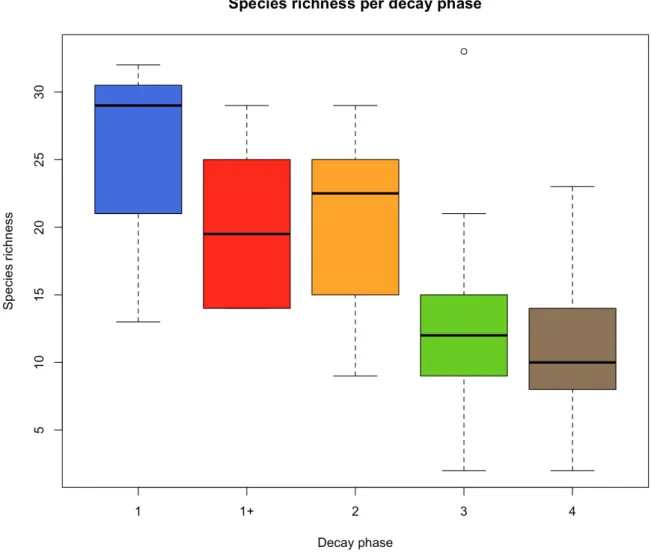
Figure 5. Boxplots of total species richness per decay phase

Figure 5 shows the mean number of species per decay phase, grouped in Quartiles and with the black line indicating the median. This is the total species richness, including the corticoid species. Just like Figure 3 and Figure 4, the boxplots with- and without corticoid species show the same trends, only a lower absolute number. Table4 shows the mean species richness per decay phase with the associated standard deviation and variance.

Decay phase 1 has the highest species richness, followed by decay phase 2 and 1+. Decay phases 3 and 4 show the lowest species richness.

(26)

DECAY STAGE MEAN STANDARD DEVIATION VARIANCE 1+ 20.167 6.911 47.767 1 24.667 10.214 104.333 2 19.700 6.913 47.789 3 12.098 5.607 31.440 4 10.938 4.220 17.805

Table 4. Mean number of species, standard deviation and variance per decay stage

Because decay stage 1 only comprised three logs and decay stage 1+ only six, we grouped them together under ‘decay stage 1’.

Figure 6. Species richness per decay stage with 1+ and 1 grouped together

Again, decay stage 1 has the highest species richness, followed by decay stage 2.

DECAY STAGE MEAN STANDARD

DEVIATION VARIANCE

1 21.667 7.810 61.000

2 19.700 6.913 47.789

3 12.098 5.607 31.440

4 10.938 4.220 17.805

(27)

Statistical test: significant differences in species richness due to decay stages?

In order to test whether there is a significant difference in species richness due to decay stages, in other words to perform an ANOVA, we need to test the assumptions:

1) the residuals need to be Normal distributed (if this is not the case, we check all subsets of the data individually)

2) all variances need to be homogenous.

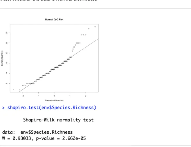
The first ANOVA is conducted with all species, the second ANOVA without corticoids. 1. test whether the data is Normal distributed

Figure 7. QQ-plot and Shapiro-Wilk normality test of the species richness

The p-value of the Shapiro-Wilk normality test is smaller than 0.05, which means the data is not normally distributed. Subsets per decay stage are made, which all need to be non-significant in a Shapiro-Wilk normality test in order to perform an ANOVA test. All subsets are normally distributed except decay phases 1+ and 3. After grouping 1 and 1+, only decay phase 3 tests significant.

(28)

Figure 8. Output of the Shapiro-Wilk normality test for decay phase 3

After sqrt-transformation of the whole data the p-value is larger than 0.05.

Figure 9. Output of Shapiro-Wilk normality test after sqrt-transformation

2. test whether the variances are homogenous

Figure 10. LeveneTest to check homogeneity of variances

After performing a leveneTest to check the homogeneity of variances, the p-value > 0.05. This means that indeed the variances are homogenous and we can use a parametric test to test for differences between decay stages.

3. performing a one-way ANOVA

H0: There is no significant effect in species richness between decay stages. HA: There is a significant effect in species richness between decay stages.

An ANOVA type III test is chosen to correct for marginal effects, because not all groups (decay stages) are equally large. With this ANOVA we test whether there is a significant effect of decay stage on species richness.

(29)

Figure 11. ANOVA type III test

The p-value gives the chance that H0 is correct and here it is << 0.05 (= 1.003 * 10-6_{). This} means that we reject the null hypothesis and conclude that there is a significant effect of decay stage on species richness.

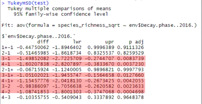
To determine which decay stages exactly differ in species richness, a post-hoc test (Tukey test) is applied. This renders a matrix in which a p-value is given for each comparison of two different decay stages. A p-value < 0.05 indicates that there is a significant difference in species richness between the two respective decay phases. Significant p-values are indicated in the red box.

(30)

The Tukey test shows that there is a significant difference in species richness between decay stages: 3 – 1, 4 – 1, 3 – 1+, 4 – 1+, 4 – 2. When roughly interpreted we see a significant difference between early and late decay stages.

Now, the same steps are repeated but without the corticoid species. 1. test whether the data is Normal distributed

Figure 13. Output of the shapiro test without corticoid species

Even without corticoid species the dataset is still not Normal distributed (p < 0.05). We now make subsets of each decay stage and test whether these are Normal distributed.

Figure 14. Output of the shapiro test for decay stage 3 (1 and 1+ grouped)

After grouping decay stages 1 and 1+, only decay stage 3 is not Normal distributed.

Figure 15. Output of the shapiro test when squared-transformed

After sqrt-transformation the data is Normal distributed and we can perform an ANOVA. 2. test whether the variances are homogenous

(31)

The p-value > 0.05, which means the assumption of homogeneity of variances is correct. 3. performing a one-way ANOVA

Figure 17. Output of the ANOVA test

The p-value gives the chance that H0 is correct and here it is << 0.05 (= 9.896 * 10-7_{). This} means that we reject the null hypothesis and conclude that there is a significant effect of decay stage on species richness.

Figure 18. Output of the Tukey test, significant differences are indicated in red

In the dataset without corticoid species we see the same trend as when corticoid species are included: significant differences in species richness between young and old decay stages.

(32)

Abundances

Only five species (2,2%) were recorded on more than 50 logs:

Hypholoma fasciculare (Huds.) P. Kumm. (79), Botryobasidium subcoronatum (Höhn. &

Litsch.) Donk (73), Pluteus cervinus (Schaeff.) P. Kumm. (59), Kretzschmaria deusta (Hoffm.) P.M.D. Martin (57) and Mycena galericulata (Scop.) Gray (55). Only 14,6% of all species occur on 10 or more logs. 105 out of 223 species (47,3%) are singletons, 33 species (14,6%) are doubletons.

Below are four rank-abundance plots visualizing the number of counts per species in decreasing order. The first plot comprises all 223 species, the second plot all species except the corticoids (except the few common ones that were also counted in the NAT-MAN project). On these graphs both species richness and evenness can be seen. Species richness is the amount of species on the x-axis and species evenness is the slope of the decreasing curve. The next two plots (Figure 19b) are a comparison between 2001 and 2018. The 2018 plot is the same as in Figure 19a, repeated to make an easier comparison.

Both rank abundance plots have a long tail, which emphasizes many rare species. The curve that can be visualized on the bars follows a log-series model.

(33)

dan ce p lo ts o f a ll sp ec ie s, and a ll spe ci es e xc ep t c or tic oi ds

(34)

Figu re 1 9b. R an k-abun dan ce p lo ts o f 2001 (193 lo gs ), an d 2018 (10 8 lo gs , n o co rt ic oi ds )

(35)

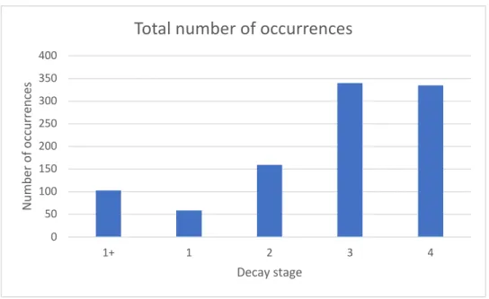
Figure 20. Number of occurrences of all species excluding the corticoids

Figure 21. Number of occurrences of all species, including the corticoids

Figure 20 and figure 21 show the number of occurrences per decay stage. As mentioned earlier, “1” occurrence is represented by one species on one tree. E.g. when 10 fruitbodies of

Hypholoma fasciculare occur on a single log, this is mentioned as 1 occurrence.

Interestingly, we saw earlier that the youngest decay stages show the highest species richness. Here, we see that the oldest decay stages show the highest number of occurrences. This means that in the older decay stages there are less different species, but more occurrences of the same returning species.

0 50 100 150 200 250 300 350 400 1+ 1 2 3 4 Nu m be r o f o cc ur re nc es Decay stage

Total number of occurrences

0 100 200 300 400 500 600 1+ 1 2 3 4 Nu m be r o f o cc ur re nc es Decay stage

(36)

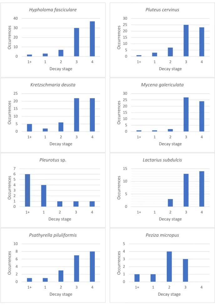
Figure 22. Occurrences per decay stage of specific species 0 10 20 30 40 1+ 1 2 3 4 Oc cu rr en ce s Decay stage Hypholoma fasciculare 0 5 10 15 20 25 30 1+ 1 2 3 4 Oc cu rr en ce s Decay stage Pluteus cervinus 0 5 10 15 20 25 1+ 1 2 3 4 Oc cu rr en ce s Decay stage Kretzschmaria deusta 0 5 10 15 20 25 30 1+ 1 2 3 4 Oc cu rr en ce s Decay stage Mycena galericulata 0 1 2 3 4 5 6 7 1+ 1 2 3 4 Oc cu rr en ce s Decay stage Pleurotus sp. 0 5 10 15 1+ 1 2 3 4 Oc cu rr en ce s Decay stage Lactarius subdulcis 0 2 4 6 8 10 1+ 1 2 3 4 Oc cu rr en ce s Decay stage Psathyrella piluliformis 0 1 2 3 4 5 1+ 1 2 3 4 Oc cu rr en ce s Decay stage Peziza micropus

(37)

Figure 22 shows the occurrences per decay stage of different fungi. The selection is based on a high number of occurrences, a variety of taxonomic groups and preference for different decay stages.

Fungal community composition

The previous part focused on the species richness, while this part evaluates the community structure. The recorded fungi are linked with environmental variables related to the logs. To what degree do the environmental variables explain the data? Previously it was shown that there is a significant effect in species richness between the young decay stages and the old decay stages, but this explains nothing about the composition or a potential shift in community composition. Previous research on the same logs by Walleyn & Vandekerkhove (2002) has shown that decay stage is an important variable in explaining the fungal community composition.

1. Indicator analysis

The indicator analysis tries to answer the research question:

4) Are there species that perform an indicator function for certain decay stages?

To understand if certain species are bound to specific decay stages, an indicator analysis is performed. This analysis produces a list of species for each decay stage with accompanying indicator values. The R script can be found in Appendix 4.

(38)

Figure 23. Results of the indicator species analysis

Figure 24. Results of the indicator species analysis, for decay stages 1 and 1+ together

Figure 23 shows the output of the indicator analysis (Cáceres 2013). Three groups can be seen, which represent the decay stages: Group 1, Group 1+ and Group 2. Below each group is a list

(39)

of species, with their specific indicator values to the right. Apparently, the program renders it impossible to determine indicator species of decay stages 3 and 4. Even when stages 3 and 4 are grouped together, no indicator species are found. Figure24 shows the indicator species for decay stages 1 and 1+ together.

Column A states the chance that a log belongs to the respective decay stage given that the species occurs on that log. A value of 1 means that this species is only found in this decay stage. Column B represents the chance that the species is found on a log belonging to the respective decay stage. A value of 1 would mean that this species is present on every log of the specific decay stage.

The column stat gives the product of columns A and B. The column p-value gives the significance of the proposed indicator species.

Keep in mind that decay stage 1 only comprised three logs and decay stage 1+ only six logs. Apparently, Hypoxylon multiforme (Fr.) Fr. occurred on all six logs of decay stage 1+ and not at all on decay stage 1, while Hypoxylon fragiforme (Pers.) J. Kickx f. only occurred on decay stage 1. Functional groups 0 20 40 60 80 100 120 140 1+ 1 2 3 4 Nu m be r o f s pe ci es

Number of species per functional group per decay stage

St Am Pb Sh Pn Em

(40)

Figure 25 represents the distribution of functional groups over the decay stages. The legend is explained as follows:

Abbreviation Functional group

St Terrestrial saprotrophic

Am Association with moss

Pb Biotrophic parasite

Pn Necrotrophic parasite

Sh Wood saprotrophic

Em Ectomycorrhizal

Table 6. Legend of functional groups

Wood decomposers (Sh) make up the largest fraction over all decay stages. Together with necrotrophic parasites (Pn) they are a constant representation over all the decay stages. From decay stage 2 onwards ectomycorrhizal species start to appear, the same for terrestrial saprotrophic species. The group of association with mosses is present from decay stage 1 onwards, but the size of this group never exceeds 4 species. Only one biotrophic parasite (Cordyceps militaris (L.) Fr.) was found, decay stage 4.

(41)

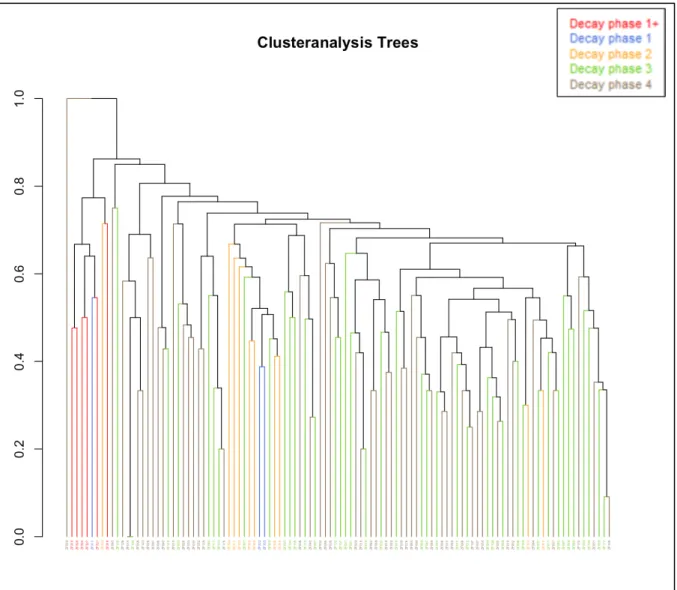
Cluster analysis

(42)

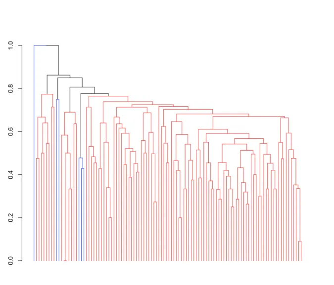
Figure 27. Result of SIMPROF test, significant clusters are alternated red and blue

Figure 26 represents the result of the cluster analysis in R, comparing the community composition on each log. Each branch represents a log, in the same colors as indicated in the beginning. Here we see that decay stages 3 and 4 form intermixed clusters, while decay stages 1+, 1 and 2 are separated. Decay stage 1 is divided over the clusters from 1+ and 2, which means that the community composition of stage 1 is similar to either 1+ or 2.

Figure 27 represents the result of the SIMPROF analysis in R. This test shows where the clusters differ significantly between each other, alternatingly indicated in red and blue. The uttermost left branch represents ZF029, which appears to be significantly different from all the other logs. Next, we have a cluster that is significantly different, indicated in red. When looking at the cluster analysis tree it is clear that this group comprises logs of early decay stages (all the logs from 1+, with one log from decay stages 1 and 2 each).

(43)

Environmental variables

This part focuses on the research question:

6) To which extent do the measured environmental variables explain the structure in the fungal community?

Figure 28. Pairwise correlations between the different variables and decay stage

Figure 28 shows the pairwise correlations between different environmental variables. The dataset with all species is included, including corticoids. On the diagonal a histogram is given for the values of each variable. On the left side of the diagonal scatterplots are given for the combination between the two variables that intersect on the graph. The numbers on the right side of the diagonal are correlation coefficients for, again, the two variables that intersect in that box. The higher the correlation between two variables, the higher the number.

(44)

on CWD, volume and decay stage where the most apparent factors explaining species richness (Heilmann-Clausen & Christensen 2003).

Figure 29. Pairwise correlations between species richness and chemical parameters

Figure 29 shows pairwise correlations between species richness and chemical parameters inside the logs.

(45)

Ordination analyses

Figure 30. CA analysis of all species

Figure 30 is the result of a CA analysis with all species included. After a first exploratory CA analysis, we decided to remove ZF159 (decay stage 4) to allow a more even spreading of the other data. The species compositions of decay stage 1 are more different than the bulk of the logs comprising decay stages 2, 3 and 4.

(46)

(47)

Figure 31 shows the result of a CCA analysis of all species with forward selection of explaining variables. The incorporated variables include decay phase, volume of the log, C content, N content, C:N ratio, percentage moss coverage.

The forward selection generated a p-value for each variable and three variables came out as significant: decay stage 1+, N content, C content.

Analysis ‘Constrained’ – Forward selection results

Explains % Contribution % pseudo-F p-value

Decay phase (1+) 4.2 13.9 2.9 00.1

N 2.1 6.9 1.5 0.002

C 1.9 6.4 1.4 0.004

Table 7. Explaining variables in species composition

Figure 32 shows the result of a NMDS analysis with all species, but a restricted dataset (i.e. no singletons, no doubletons, no logs with < 5 species). This restricted dataset was used because the complete dataset rendered too much noise and the stress levels were too high (> 0.20 for Sorensen and Jaccard). However, with this restricted dataset the stress level is still too high (0.21). The labels represent the logs, colored by decay phase.

(48)

(49)

Analysis ‘Constrained’ – Forward selection results

Decay phase (1+) 6.7 18.8 4.5 0.002

Decay phase (1) 3.5 10.0 2.4 0.002

Decay phase (2) 2.8 7.8 1.9 0.002

C 2.1 6.0 1.5 0.01

Table 8. Explaining variables in CCA analysis with forward selection

Now, the same procedure is repeated but without the corticoid species (except the most common ones). An exploratory CCA analysis showed that ZF038 prevented an even spread of the data. We decided to remove ZF038.

(50)

Figure 34. CCA analysis of the restricted dataset without corticoid species Analysis ‘Constrained’ – Forward selection results

Decay phase (1+) 7.0 20.6 4.5 0.002

Decay phase (1) 3.7 10.8 2.5 0.002

Moss coverage 2.2 6.3 1.4 0.006

Decay phase (2) 2.4 7.1 1.6 0.006

Table 9. Explaining variables in CCA analysis with forward selection

Figure 34 shows the CCA analysis of the restricted dataset without corticoid species, with forward selection of explaining variables. Four variables were shown to contribute significantly to the species composition: decay phases 1+, 1 and 2 and moss coverage.

(51)

Figure 35. NMDS of the restricted dataset without corticoid species

Figure 35 shows the result of a NMDS analysis of the restricted dataset (i.e. no singletons, no doubletons, no logs with < 5 species) without corticoid species. The young decay stages seem to cluster together, but the stress level is 0.2 which means we need to be careful with interpreting the results.

Succession

In this part we try to answer the following question:

2) Is there a change in fungal community composition related to the successive pattern of decay stages?

Figure 36 is the result of a NMDS for the dataset without corticoid species, combined with the dataset from 2001. ZF050 and ZF053, both from 2001, are removed from the dataset as they prevent a clear view of the spreading. The stress level is < 0.20 which makes this graph safe for interpretation.

(52)

representation of the change in fungal species composition related to progressing decay stages.

Figure 36. NMDS of a combined dataset from 2001 and 2018

A clear distinction in species composition can be seen between 2001 and 2018. This means the communities within each year cluster more together than that each tree clusters with its younger/older self. Whether this is due to a successional pattern or due to less species per tree because of (or) environmental patterns (the weather) will be discussed in the discussion.

(53)

Change in community composition

In this part the following question will be addressed:

3) Is there a change in the overall fungal communities within each decay class after 17 years? We will compare the subset of beech logs in their different decay stadia from Walleyn & Vandekerkhove (2002) to a contemporary similar subset. The aim is to investigate whether the fungal diversity of the beech logs has changed over the years.

2018 2001 1 9 9 2 10 9 3 40 48 4 20 19 TOTAL 79 85

Table 10. Number of beech logs per decay stage

After an exploratory NMDS we decided to remove ZF050 and ZF053 (both from 2001, decay stage 1) to allow an even spread of the other logs.

(54)

Figure 37. NMDS of a combined dataset from 2001 and 2018, with similar subsets of logs in decay stages

Figure 37 is the result of a NMDS of a combined dataset from 2001 and 2018. The stress level is < 0.18, which makes this graph safe for interpretation. We see a clear separation between the logs from 2001 and 2018. This means the communities cluster more within one year, than that they cluster per decay stage.

(55)

Figure 38. NMDS of decay stages 1 and 2 from 2001 and 2018

To illustrate this more clearly, figure 38 shows the clustering species compositions from decay stages 1 and 2. The different years are indicated with 2001 as stages 1’ and 2’ in lighter colors and 2018 in the style used throughout the thesis. We still see a seperation between 2018 on the upperside and 2001 on the downside. If the communty compositions within the decay stages would be more alike, the yellow symbols would cluster together and the blue symbols would cluster together. This is not the case.

Figure 39 gives the same illustration as figure38, with all decay stages added. Decay stages from 2001 are indicated with an apostrophe and lighter shades of the same colors.

Decay stage 1 (blue) seems to cluster together. The older decay stages cluster by year.

(56)

Comparing species

Below, a list of species from 2018 that were not recorded in 2001 (without corticoids species).

Apioperdon pyriforme Chlorophyllum rhacodes Clitocybe nebularis Cordyceps militaris Crepidotus applanatus Crepidotus variabilis Cudoniella aciculare Gymnopus dryophila Hygrophoropsis aurantiaca Hypoxylon multiforme Inocybe geophylla Laccaria amethystina Laccaria proxima Lactarius blennius Laetiporus sulphureus Lenzites betulinus Marasmius alliaceus Mucidula musida Mycena cinerella Mycena inclinata Mycena pseudocorticola Mycena speirea Paxillus involutus Polyporus brumalis Polyporus squamosus Polyporus varius

Psathyrella artemisiae var. artemisiae Psathyrella senex Rickenella setipes Rimbachia arachnoidea Ripartites tricholoma Russula atropurpurea Russula cfr. persicina Russula fellea Schizopora flavipora Schizopora paradoxa Schizopora radula

(57)

Old-growth (beech) forest indicator species

In this part we address the question:

5) Are there species that perform an indicator function for old-growth forests and/or beech forests?

Dvorak et al. (2017) provided a list of indicator species for old-growth forests (Dvořák et al. 2017). The species that were observed during our surveys are listed here: i.e. Mycena hiemalis (Osbeck) Quél., Mycena laevigata Gillet, Peziza micropus Pers., Phleogena faginea (Fr.) Link,

Pluteus hispidulus (Fr.) Gillet, Pluteus nanus (Pers.) P. Kumm, Pluteus phlebophorus (Ditmar)

P. Kumm, Pluteus Plautus Quél., Pluteus podospileus Sacc. & Cub., Pseudoclitocybe

cyathiformis (Bull.) Singer. Below, a selection of six interesting indicator species are depicted.

All species here discussed have Fagus as substrate preference.

Pluteus hispidulus (Fr.) Gillet, Pluishoedhertenzwam

Systematic position: Basidiomycota, Agaricales

Description: Cap < 25 mm diam., dark grey to brown grey. Gills free, whitish to pink. Stipe < 40 mm long. Pileipellis cutis. Pleurocystidia rare to absent.

Ecology: Terrestric saprotrophic Phenology: Late summer to autumn

Observations: 25/09 (2x), 7/10, 13/10 (2x), 27/10 Identification key: (Vandeven 1990)

Notes: Cap more fibrous and habitus smaller than Pluteus ephebeus.

(58)

Pluteus nanus (Pers.) P. Kumm, Dwerghertenzwam

Description: Cap 20 – 50 mm diam., young conical to convex later, dark grey to brown grey. Gills free, young whitish to later (brownish) pink. Stipe 40 – 50 x 5 – 10 mm, white to striped grey to completely grey with white flakes. Pileipellis hymeniderm, cells club-shaped to sferopedunculate (Q < 3). Pleurocystidia small utriform to long egg-shaped. Caulocystidia present. Spores round to elliptic, orange brown, 6.3 – 8.5 x 5 – 7.1 µm.

Ecology: Wood saprotrophic Phenology: Summer to autumn

Observations: 16/09, 17/09 (2x), 25/09, 13/10 (2x), 20/10, 27/10, 15/11 Identification keys: (Vandeven 1990), (Breitenbach & Kränzlin 1995)

(59)

Pluteus plautus Quél., Knolvoethertenzwam

Description: Cap 20 – 50 mm diam., young conical to convex later, dark grey to brown grey, white in

Pluteus plautus incl. semibulbosus. Gills free, young whitish to later (brownish) pink. Stipe 20 – 30 x

2 – 4 mm, flaky from caulocystidia. Pileipellis hymeniderm, cells cylindric to spindle-shaped (Q > 3), 80 – 240 x 10 – 30 µm. Pleurocystidia abundant. Caulocystidia present. Spores round, smooth, brown red, 6.3 – 9.3 x 5.6 – 8.3 µm.

Ecology: Wood saprotrophic

Phenology: Early summer to autumn

Observations: 25/09 (2x), 7/10, 13/10 (2x), 27/10

Identification keys: (Vandeven 1990), (Breitenbach & Kränzlin 1995)

Notes: According to the literature Pluteus semibulbosus is a synonym of Pluteus plautus. However,

P. semibulbosus has a white to crème cap.

(60)

Pluteus phlebophorus (Ditmar) P. Kumm., Geaderde hertenzwam

Description: Cap 15 –40 (50) mm diam., young conical to convex later, brown to dark brown, veined to fine veined. Gills free, young whitish to later pink. Stipe 20 – 30 (40) x 2 – 4 mm, smooth.

Pileipellis hymeniderm, cells club-shaped to sferopedunculate (Q < 3), 30 – 60 x 13 – 34 µm. Pleurocystidia abundant. Spores round to elliptic, smooth, 5.9 – 8.4 x 5.6 – 7.1 µm.

Ecology: Wood saprotrophic

Phenology: Early summer to autumn Observations: 16/09, 17/09 (3x)

Image4. Cap, stipe and gills of Pluteus phlebophorus (JG-18-019, 16/09/2018)

Image5. Pileipellis of Pluteus phlebophorus (magnification 20x10x), (JG-18-077, 17/09/2018). Note the club-shaped cells (arrow)

(61)

Pluteus podospileus Sacc. & Cub., Fluweelhertenzwam

Description: Cap 8 - 10 (20) mm diam., young conical to convex later, often irregular shaped, finely

craquelé in centre, dark brown, dry, velvet touch. Gills free, young whitish to later (brownish) pink.

Stipe 30 – 40 (40) x 2 – 3 mm, smooth or flaky. Pileipellis hymeniderm, 2 types of cells: spindle-shaped and club-spindle-shaped. Pleurocystidia abundant. Spores round, 5.1 – 7.3 x 4.8 – 6.7 µm. Ecology: Terrestric saprotrophic

Phenology: Summer to autumn Observations: 16/09, 20/10

50 µm

(62)

Pseudoclitocybe cyathiformis (Bull.) Singer, Bruine schijntrechterzwam

Description: Cap deeply depressed, inrolled at the margin, dark brown. Gills decurrent, crowded, pale greyish. Cystidia absent. Spores 8 – 12 x 5 – 6.5 µm, smooth, amyloid.

Ecology: Terrestric saprotophic

Phenology: Late summer to early spring

Observations: 13/10, 20/10, 4/11, 15/11 (2x), 17/11 (2x), 30/11, 18/12, 20/12

Notes: While this species was not as abundant as many others, it was however one of the few species that kept occurring until the last inventories (late December).

(63)