RIVM Report 2015-0095
A.M.A. van der Linden et al.
Evaluation of the Dutch
leaching decision tree with
the substances bentazone,
MCPA and mecoprop
Page 2 of 96
Colophon
© RIVM 2015
Parts of this publication may be reproduced, provided acknowledgement is given to: National Institute for Public Health and the Environment, along with the title and year of publication.
A.M.A. van der Linden (author), RIVM W.H.J. Beltman (author), Alterra J.J.T.I. Boesten (author), Alterra J.W. Pol (author), Ctgb
Contact:
Ton van der Linden RIVM
Ton.van.der.Linden@RIVM.nl
This investigation has been performed by order and for the account of the Ministry of Infrastructure and the Environment and the Ministry of Economic Affairs, within the framework of the projects ‘Verkenning en Evaluatie gewasbescherming’ and ‘Beoordelingsmethodieken Toelating Gewasbeschermingsmiddelen’.
This is a publication of:
National Institute for Public Health and the Environment
P.O. Box 1 | 3720 BA Bilthoven The Netherlands
Synopsis
Evaluation of the Dutch leaching decision tree with the substances bentazone, MCPA and mecoprop
The leaching of bentazone, MCPA and mecoprop to groundwater was assessed using the new proposals for evaluating sorption and
degradation studies (Boesten et al. 2015). The three substances are weak acids, showing pH-dependent sorption behaviour in soil. The evaluation led to large corrections for the sorption endpoint, KOM, derived for individual studies. Consequently, the curve describing sorption as a function of soil pH changed, indicating lower sorption over the relevant pH range. None of the available Freundlich exponents passed the reliability check.
Using the improved interpretation procedures for sorption and
degradation experiments revealed that several usages of the substances did not comply with the threshold limit for leaching when assessed at both Tier 1 and Tier 2 of the decision tree on leaching. The assessments did not reveal shortcomings in the decision tree itself. It is
recommended that the improved interpretation procedures for sorption and degradation experiments are used for deriving endpoints for future substance leaching evaluations.
Keywords: degradation, drinking water, plant protection products, risk assessment, sorption
Publiekssamenvatting
Evaluatie van de beslisboom voor uitspoeling van bentazon, MCPA en Mecoprop
Evaluatie Beslisboom Uitspoeling Gewasbeschermingsmiddelen naar grondwater
Sinds 2004 wordt een beslismodel (beslisboom) gebruikt om te
beoordelen in welke mate een gewasbeschermingsmiddel uitspoelt naar het grondwater. Uit een evaluatie van het RIVM, het College voor de toelating van gewasbeschermingsmiddelen en biociden (Ctgb) en onderzoekinstituut Alterra blijkt dat de beslisboom goed werkt en state of the art is. Wel laten de stofgegevens waarmee wordt gerekend te wensen over. Om de kwaliteit van het grondwater te waarborgen moeten deze gegevens zorgvuldiger worden afgeleid.
Drinkwaterbedrijven hebben gevraagd om het beslismodel te evalueren, omdat zij betwijfelen of het grondwater afdoende wordt beschermd. In grondwaterbeschermingsgebieden gelden extra strenge normen voor het gebruik van gewasbeschermingsmiddelen. In grondwater worden soms restanten van gewasbeschermingsmiddelen teruggevonden. Dit betreft voornamelijk stoffen die inmiddels zijn verboden. Ze zijn zeer
waarschijnlijk in het verleden gebruikt en door de jaren heen in de ondergrond onvoldoende afgebroken.
Het blijkt dat een aantal stoffen sneller door de bodem wordt
getransporteerd dan op grond van de huidige afleidingsmethodiek wordt verwacht. Hierdoor is er minder tijd beschikbaar voor afbraak in de bodem. Met de huidige afleidingsmethodiek voor de stofgegevens wordt dan een te lage uitspoeling berekend en daardoor te lage concentraties in het grondwater. De onderzoekers hebben voorstellen gedaan voor een zorgvuldiger afleiding van stofgegevens voor het beslismodel. De voorgestelde procedures daarvoor zijn beschikbaar in een ander rapport. Door toepassing van deze procedures worden hogere concentraties voor stoffen in het grondwater voorspeld. Voor de drie onderhavige stoffen kan dat aanvullende beperkingen voor de toelating opleveren, wat leidt tot lagere concentraties van deze middelen in het milieu.
Kernwoorden: afbraak, bestrijdingsmiddelen, degradatie, drinkwater, risicobeoordeling, sorptie
Contents
Summary — 9 1 Introduction — 11 2 Bentazone — 15
2.1 General information on bentazone — 15 2.2 Sorption — 15
2.2.1 Batch and TLC studies — 15 2.2.2 Soil column studies — 18
2.2.3 Combination of batch, TLC and soil column studies — 21 2.3 Degradation — 23
2.3.1 Laboratory studies — 23 2.3.2 Field studies — 24
2.3.3 Combination of field and laboratory DegT50 values — 33 2.4 Selected usages and assessment — 34
3 MCPA — 39
3.1 General information on MCPA — 39 3.2 Sorption — 39
3.2.1 Selection of MCPA sorption coefficients — 40 3.2.2 Selection of the Freundlich exponent values — 49 3.2.3 Conclusions sorption — 49
3.3 Degradation — 50
3.3.1 Conclusions degradation — 51
3.4 Selected usages and assessment — 51
4 Mecoprop — 57
4.1 General information — 57 4.2 Sorption — 57
4.3 Degradation — 62
4.4 Selected usages and assessment — 63
5 Discussion, conclusions and recommendations — 69
5.1 Bentazone — 69 5.2 MCPA — 71 5.3 Mecoprop — 72
5.4 Overall conclusions — 74
5.5 Recommendations for further research — 75
References — 77
Appendix A Glossary — 83
Appendix B Details of MCPA studies — 85
Appendix C References concerning MCPA considered not useful/relevant for this evaluation — 91
Summary
Occasionally, residues of plant protection products have been found in groundwater in concentrations above the drinking water threshold level. This led to the question whether the groundwater is protected
sufficiently by the procedure laid down in the decision tree on leaching of 2004. Therefore, the decision tree was evaluated by assessing the leaching of bentazone, MCPA and mecoprop to groundwater, using the new proposals for evaluating sorption and degradation studies (Boesten et al. 2015).
The three substances are weak acids, showing pH-dependent sorption behaviour in soil. Applying the new proposals for evaluating fate studies led to large corrections for the sorption endpoint, KOM, for individual studies and consequently for the curve describing the dependency on soil pH. Corrections of more than 50% were found for 9 out of 10
sorption values for bentazone, 7 out of 28 for MCPA and 13 out of 20 for mecoprop.
Applying the proposed quality check for the Freundlich sorption exponent N led to the conclusion that none of the evaluated N values could be considered acceptable. Therefore, the default value of 0.9 was used in subsequent evaluations.
Tier 1 leaching calculations showed leaching concentrations above the drinking water threshold limit for all three substances. Tier 2 calculations for bentazone also showed concentrations above this limit. Using the current approach (FOCUS 2006), calculations for MCPA and mecoprop led to concentrations below the limit except for one mecoprop case with an adjusted half-life. Applying the proposed EFSA (2012) approach resulted in exceedances of the limit for applications after 1 June for MCPA and after 1 September for mecoprop. Calculations with the adjusted half-life for mecoprop resulted in an exceedance for the application in March as well. Calculations for historical applications in October showed exceedances for all three substances.
The evaluation revealed that concentrations above the drinking water threshold limit could have been expected for several uses of the three substances if the new proposals for evaluating sorption and degradation experiments had been applied. Using the new proposals in combination with the current decision tree would probably change some
authorisations and ensure better protection of groundwater.
Including data from published literature had no influence on the DegT50 endpoint for all three substances. Its inclusion had a negligible influence on the KOM–pH relationship for bentazone (admittedly, the ‘published literature’ consisted of only three KOM values, as measured by the RIVM and Alterra for three Dutch soils). In contrast, the published literature had considerable influence for MCPA and some effect for mecoprop. Adding published data led to an increase of the KOM in the most important part of the KOM–pH curve and is therefore expected to
Page 10 of 96
Our simulations for mecoprop and MCPA (applications on a well-developed grass cover) showed that use of the default parameters for wash-off and degradation on plant surfaces as recommended by EFSA (2012) may lead to a considerable increase in evaluated leaching concentrations in comparison with the current approach.
Our GeoPEARL simulations for bentazone showed that GeoPEARL is not suitable for simulating wash-off from plant surfaces. Since GeoPEARL is hydrologically based on only three crops (maize, potatoes and grass), it does not simulate wash-off realistically.
The quality criteria for the Freundlich exponent (which led to the
rejection of all reported values for this exponent) have a weak scientific basis. We therefore recommend underpinning or improving these criteria by means of an analysis of the error in this exponent.
The new proposal for interpreting indirect batch sorption studies, i.e. using a default correction factor of 10% degradation/loss, sometimes appeared overly conservative in the light of other evidence. This 10% is a conservative value based on the requirement in OECD106 (OECD 2000) to achieve at least 90% recovery of the test substance. We therefore recommend performing a literature review on the relationship between the degradation rate in batch systems and the degradation rate in soil or water-sediment studies, which is likely to allow a less
1
Introduction
Assessment of the leaching of plant protection products (PPP) to groundwater has been part of the authorisation process in the
Netherlands since environmental factors were explicitly included in the risk assessment procedures. In the late 1980s and early 1990s it
became clear that protecting groundwater as a source of drinking water is the specific protection goal of the assessment procedure. This has been laid down in both the Dutch law on pesticides and related guidance (WGB 2007; Van der Linden et al. 2004).
The principles of the current leaching assessment procedure were laid down in the ‘new decision tree on leaching’ (Van der Linden et al. 2004), while many practical aspects are covered in the leaching models PEARL and GeoPEARL (Leistra et al. 2001, Tiktak et al. 2000, Tiktak et al. 2003) and leaching scenarios (FOCUS 2000, FOCUS 2009). The
assessment follows a tiered approach (Figure 1-1), where Tier 1 is fully harmonised with procedures at the European level and Tier 2 and Tier 3 are more specific to the Netherlands. In all tiers, it is assessed whether the concentrations in groundwater under realistic worst-case conditions exceed the threshold limit for PPP and relevant metabolites in drinking water. The decision criterion in Tier 2 is more explicitly defined as follows: ‘the annual average concentration in the groundwater at 1 m depth should not exceed the drinking water threshold level in at least 90% of the potential area of use.’ Tier 3 considers transformation in the groundwater between 1 m and 10 m depth and the above criterion should be met at 10 m depth. A stricter criterion is applied for PPP intended to be used within groundwater protection areas.
Page 12 of 96
Drinking water companies and provinces in the Netherlands monitor groundwater (and other environmental compartments) for the
occurrence of active substances and metabolites of PPP. Occasionally, residues have been found in concentrations that are above the drinking water threshold level (see for example Van der Linden et al. 2007, Arts et al. 2006). This led to the question whether groundwater is sufficiently protected by the procedure laid down in the new decision tree (Van der Linden et al. 2004). The Ministries of Infrastructure and the Environment (IenM) and Economic Affairs (EZ) therefore initiated a project in order to examine whether the decision tree on leaching of PPP and related
metabolites adequately meets the specific protection goal. The research is not to be seen as validation of the decision tree because the correct functioning of the decision tree was not checked against independently derived (monitoring) data, of which the position (ranking) on the cumulative probability density function with respect to leaching is known.
Tier 3 of the decision tree was not evaluated because (1) this tier is only exceptionally used in risk assessment, and (2) it would require a
considerable amount of time to determine the representativeness and ranking of the monitoring wells on the cumulative probability density function. This was not considered to be an efficient use of the resources of the workgroup.
At the start of the project, it was considered impossible to establish the representativeness of the wells with sufficient certainty, as past usage patterns, i.e. at the time of infiltration, cannot usually be reconstructed adequately. Consequently, Tier 3 of the decision tree was excluded from this evaluation.
The initial phase of the project identified the PPP substances that are found most frequently in groundwater and are still on the market, as these were considered to be the most worthwhile substances to use in the assessment. The working group identified these as bentazone, MCPA and mecoprop. Substances found in groundwater but taken off the market because of a negative decision with regard to leaching were considered not suitable for testing the decision tree, as, in theory, they would fail to meet the leaching criterion (Boesten et al. 2011). The next phase of the project revealed a number of methodological issues with regard to important input variables in the leaching assessment: the degradation and sorption parameters. The working group decided to address those issues first and recommended several changes in the interpretation of sorption and transformation experiments as well as in the parameters for use in leaching assessments (Boesten et al. 2011). In the last phase of the project, the working group addressed the basic question: ‘Is the decision tree fit for purpose?’, applying the changed methodologies developed in the earlier phase. The results of this phase are reported here. As deriving pesticide fate characteristics appeared to be critical, the derivation of this data is described separately for each of the test substances (see Chapters 2–4 and the accompanying
workbooks). A study of the relevant dossiers and published literature revealed several weaknesses in the proposed methodologies and led to the decision to revise them slightly or describe them more clearly and
explicitly. This led to an update of the 2011 report (see Boesten et al. 2015). Conclusions as to whether the decision tree sufficiently meets the specific protection goal of safeguarding the drinking water function of groundwater are given in Chapter 5.
2
Bentazone
2.1 General information on bentazone
This section provides general information on and the physicochemical properties of MCPA according to the currently agreed List of Endpoints on bentazone (European Commission 2000).
The physicochemical properties of bentazone needed for simulation with PEARL are listed in Table 2-1.
Table 2-1 Physicochemical properties of bentazone (European Commission 2000).
Chemical name (IUPAC) 3-isopropyl-(1H)-2,1,3-benzothiadiazin-4-(3H)-one-2,2-dioxide
Molecular formula C10H12N2O3S Structural formula
Molar mass 240.3
Saturated vapour pressure 0.00017 Pa at 20 °C Solubility in water pH 3: 490 mg/L at 20 °C Dissociation constant pKa = 3.3
2.2 Sorption
2.2.1 Batch and TLC studies
Eight batch sorption values were available from Ctgb dossiers (Ctgb 2002, Ctgb 2003b); these were supplemented by three batch adsorption values taken from sorption studies by the RIVM and Alterra. All these values were established using the indirect method, i.e. the sorption constant was calculated from the decrease in concentration in the liquid phase. The table in the accompanying workbook on bentazone shows the correction procedures for the KOM and pH and their results.
(www.rivm.nl/bibliotheek/rapporten/2015-) OECD106 (OECD 2000(www.rivm.nl/bibliotheek/rapporten/2015-) prescribes
0095Bentazone_sorption_data.xlsm
not using the indirect method for determining the sorption constant when the decrease in concentration in the liquid phase is less than 20%. The decrease in concentration in nearly all the dossier studies did not comply with the OECD106 requirement, but as the studies were performed before 2000 this was not used as a deselection criterion. Figure 2-1 shows the original data points together with the corrected ones. The pH values of all the data points from the monograph (ID 1–8) were corrected because the method of the pH measurement was not reported. Figure 2-1 indicates that the correction for the possible 10% degradation had a very large effect on the estimated values; of the ten values shown, seven were corrected to zero. Combination of the
workbook with Figure 2-1B shows that the measurements by Boesten and van der Pas (2000) at pHKCl = 5.3 and by Loch et al. (1985) at pHKCl
Page 16 of 96
= 4.1 resulted in non-zero KOM values even after correction. Thus it is likely that the zero KOM values for pHKCl < 5.5 obtained from the
monograph are underestimations of the true KOM. We therefore propose to discard all zero measurements from the monograph for pHKCl < 5.5 (i.e. ID 2, 4 and 7).
A
B
Figure 2-1 KOM values for bentazone as measured in batch studies as a function of pH. Open circles are uncorrected KOM values as a function of measured pH. Closed circles are corrected KOM values as a function of pHKCl. The lines connect uncorrected and corrected pH–KOM pairs. Parts A and B differ only with respect to the scale of the vertical axis.
In view of the large uncertainties in the KOM–pH relationship and the few KOM–pH data pairs left, the soil TLC studies by Abernathy and Wax (1973) were also analysed. These authors report for all their 12 soils that the RF was 1.0 (‘bentazone moved with the water front on each of the duplicated soil plates, thus achieving an RF value of 1.0 in the soil– water system’). They provided the chromatogram of one of these studies (Pittwood soil) in their figure 2. We assumed that the centre of mass of the peak was located at the largest width of the radioactivity spot. This resulted in RTLC = 0.95. On the basis of this limited
information, we assumed that the RTLC of these 12 soils ranged between 1.0 and 0.95. K values were therefore estimated using RTLC = 0.95 with Eqn 28 of the report with θ = 0.3 and ρ =1.0 kg/L, as recommended in the report. The K values for RTLC = 1.0 are of course 0.
As described in section 3.5 of Boesten et al. (2011), the concentration in the liquid phase of the TLC study has to be estimated on the basis of applied mass and the extent of the solute dot at the end of the
experiment. From figure 2 of Abernathy and Wax (1973) we estimated a surface area of the dot of about 2 cm2. The authors report that they applied 2 µL of a solution with a radioactivity concentration of 0.01 µCi/µL (‘0.01 mCi/mL’). This is a radioactivity of 0.02 µCi. They report elsewhere in the paper a molar radioactivity of 3 Ci/mol (‘2.99
mCi/mmol’). So this 0.02 µCi corresponds to 0.007 µmol bentazone, which is about 1.7 µg of bentazone. So the bentazone concentration in the 2 µL of solution was about 0.8 µg/µL, which is 800 mg/L. The layer was 1 mm thick. So the volume of the solute dot at the end of the experiment was about 0.2 cm3 and the total concentration in the soil in the solute dot becomes 1.7 µg/0.2 cm3, or about 10 µg/cm3, which is 10 mg/L. Using a volume fraction of water of 0.6 (as recommended in the report) and a sorption coefficient of zero, this gives a concentration in the dot (cst) in the liquid phase of 16.67 mg/L. Using Eqn 25 of the report with a Freundlich exponent of 0.9 gives for cst = 16.67 mg/L that KF is 1.32 times K. This was used in estimating the KF corresponding to RTLC = 0.95.
It can be expected that the bentazone concentration in the liquid phase at the start of the experiment was an order of magnitude higher
because the spot was much smaller; this would have led to a higher cst, and thus to a lower KF when using Eqn 25.
The pHH2O values as measured by Abernathy and Wax (1973) were converted to pHKCl values with Eqn 34a of Boesten et al. (2011). Abernathy and Wax (1973) used a soil:solution ratio of 1:1, whereas Eqn 34a is based on pH measurements in systems with soil:solution ratios of 1:2 to 1:5. Therefore Eqn 34a may have led to too low pHKCl values in the low pH range (e.g. the pHH2O of 4.6 at a soil-solution ratio of 1:1 would probably have been higher if measured at a soil:solution ratio of 1:5 (Kissel et al. 2004). Therefore, we decided to average the pHH2O and pHKCl values to obtain a more realistic estimate of the true pHKCl.
Figure 2-2 shows the combined data sets of the batch and TLC studies, giving only the KOM values of the TLC studies based on RTLC = 0.95; it should be kept in mind that these values may be zero except for the one
Page 18 of 96
for the Pittwood soil (at pH = 6.1 in Figure 2-2). As discussed before, all zero batch measurements from the monograph for pHKCl < 5.5 (ID 2, 4, 7) were discarded. Considering all the TLC data in Figure 2-2, only the KOM derived from the Pittwood soil (0.246 L/kg at pH = 6.1) has added value because the uncertainty in the other TLC values is too large. Given that the KOM for this Pittwood soil is a lower limit because of the limited contact time between soil and liquid phase in TLC studies, we propose to ignore the zero KOM values from the batch studies at corrected pH values of 5.95 and 6.19 (ID 8 and 3) because of the uncertainty in the
correction of these KOM values. So only the studies ID 1, 5, 6, 9, 10, 11 and the Pittwood soil study are further considered.
Figure 2-2 The batch data points (circles) and lines of Figure 2-1B plus KOM values of bentazone based on TLC studies (triangles) by Abernathy and Wax (1973). KOM values were calculated assuming RTLC = 0.95. The pH values are averages of pHH2O and the pH values corrected to pHKCl because the correction procedure overestimates the pH shift to lower values. A photograph of the TLC plate was available only for the TLC study at pH = 6.1 (Pittwood soil).
2.2.2 Soil column studies
The data in Table 2-2 was extracted from a 1990 Dutch summary authorisation report. All studies were of soil columns 30 cm in length, with a water layer of 20 cm and a leaching time of 2 days.
Table 2-2 Characteristics of the soil column studies of bentazone. The silty sand and the loamy sand were assumed to have the same volume fraction of liquid. The pHCaCl2 values and the organic matter content are taken from a personal communication by A.M.A. van der Linden based on information in another dossier.
Nr Name of soil % leached Source Volume fraction of liquid at -10 cm pHCaCl2 Organic matter (%) Organic carbon (%) 1 Sand 2.1 99 BASF (1974a) 0.34 6.2±0.7 ? 1.23 2 Sand 2.1 100 BASF (1974b) 0.34 6.2±0.7 ? 1.23 3 Loamy sand 2.2 91 BASF
(1974a) 0.34 5.8±0.3 ? 2.26 4 Loamy sand 2.2 100 BASF
(1974b) 0.34 5.8±0.3 ? 2.26 5 Sandy loam 2.3 100 BASF
(1974a) 0.38 6.3±0.4 ? 1.02 6 Sandy loam 2.3 95 BASF
(1974b) 0.38 6.3±0.4 ? 1.02 7 Silty sand 86–94 BASF (1972) 0.34 ? 1.4
8 Sandy loam 73–88 BASF (1972) 0.38 ? 5.3 These studies were simulated using the analytical solution of Jury and Roth (1990) of the convection–dispersion equation for a semi-infinite soil column. This is strictly speaking not correct because the actual soil column had a length of 30 cm. However, this analytical solution was compared to a numerical solution for a column of 30 cm with a constant θ of 0.34, a dry bulk density of 1.5 kg/L, a dispersion length of 2.5 cm, a linear sorption coefficient of 0.06 L/kg, a DegT50 of 1000 d and 200 mm water percolation in 2 days. The numerical solution was based on the PEARL model and the thickness of the numerical compartments was 1 cm. Both the numerical and the analytical solutions showed leaching of 91% of the dosage under these circumstances. Therefore, the analytical solution was considered sufficiently accurate.
The only input parameters besides the sorption coefficient are the volume fraction of liquid (θ), the dry bulk density and the dispersion length. The dry bulk density was set at 1.5 kg/L. The solution uses the product of the dry bulk density and the sorption coefficient, so if the dry bulk density is overestimated by 10%, the sorption coefficient will be underestimated by 10%. The dispersion length was set at 2.5 cm – based on the review by Vanderborght and Vereecken (2007) – but a calculation was also made for a dispersion length of 2.0 cm.
The soil columns are freely draining. This will lead to a matric potential of about 0 cm at the bottom of the soil column and of -30 cm at the top of the soil column at the end of the leaching process. During the
leaching, it can be expected that matric potentials are closer to zero than this -30 cm. FOCUS (2000) provides estimates of moisture
Page 20 of 96
that θ at a matric potential of -10 cm is a defensible estimate of the θ during the leaching process. The values in Table 2-2 show that the estimated θ values were either 0.34 or 0.38.
As a basis for the estimation of the sorption coefficient, the sorption coefficient was calculated as a function of the percentage leached for both θ = 0.34 and θ = 0.38. Figure 2-3 shows that the sorption
coefficient decreases as the percentage leached increases (as would be expected) and that the percentages leached for a given sorption
coefficient are higher for sand (θ = 0.34) than for sandy loam (θ = 0.38). The figure shows an additional calculation with a dispersion length of 2 cm. This differed only slightly from the calculation with the dispersion length of 2.5 cm. The sorption coefficient for the respective experiments was estimated from the relationships shown in Figure 2-3 (dispersion length of 2.5 cm). Table 2-3 shows four sorption coefficients below zero, one equal to zero and three above zero ranging from 0.03 to 0.12 L/kg, together indicating no to weak sorption. The sorption
coefficients below zero may be realistic because bentazone may occur as anion and its movement may be enhanced by anion exclusion.
Figure 2-3 The sorption coefficient as a function of the fraction leached from a soil column. Calculations for sand were with a volume fraction of liquid of 0.34 and calculations for sandy loam were with a volume fraction of liquid of 0.38. Table 2-3 Sorption coefficients of bentazone estimated by inverse modelling from soil column experiments based on percentage leached.
Nr % leache Estimated sorption coefficient (L/kg)
1 99 <0 2 100 <0 3 91 0.06 4 100 <0 5 100 <0 6 95 0 7 86–94 0.03–0.09 8 73–88 0.05–0.12
The soil column studies 7 and 8 in Table 2-3 were of no use because the pH of the soils was unknown. So there is one relevant study left with a sorption coefficient above zero (0.06 L/kg). In this study 91% of a dose of 1.92 kg/ha leached with a water layer of 200 mm. Assuming that this leaching occurred in half of the water layer, this gives a leaching
concentration of 0.91 × 192 mg/m2 / 0.1 m = 1747 mg/m3 =
1.747 mg/L. The Freundlich coefficient can then be calculated by Eqn 25 of Boesten et al. (2011) with cst = 1.747 mg/L and N = 0.9. This gives a Freundlich coefficient of 0.063 L/kg. The organic carbon content was 2.26% (Table 2-2), so the organic matter content was 3.9%, which gives a KOM of 1.63 L/kg.
2.2.3 Combination of batch, TLC and soil column studies
Figure 2-4 shows all previously accepted results of batch and TLC studies plus the results of the relevant soil column studies. The upper part shows that all measured KOM values for pHKCl values above 4 are close to zero. The lower part zooms in on these low values and shows considerable scatter. This scatter is probably caused by the low
accuracy; for example, the KOM of 1.63 L/kg is based on leaching of 91% of the dose whereas the KOM of zero at pHKCl = 6.1 is based on 95% leaching (column study nr 6 in Table 2-1). These slight differences in leaching percentages may be responsible for this scatter. Therefore, there were no reasons to reject any of the data points shown in Figure 2-4.
All accepted KOM–pH pairs are listed in Table 2-4. These were fitted to Eqn 31 of Boesten et al. (2011) using the software package GraphPad Prism with a pKa of 3.3, based on the List of EndPoints (LoEP), and a molar mass of bentazone of 240.8. In the first fit the ΔpH was fitted. However, this resulted in a ΔpH of -3.4, which is not within the acceptable range given in Boesten et al. (2011). Therefore, ΔpH was fixed to the closest limit value (-0.2) in the second fit. Figure 2-4 shows that the second fit resulted in an acceptable description of the
measurements. The resulting parameters were KOM,acid = 183 L/kg and KOM,anion = 0.0 L/kg. It would have been desirable to show also the 95% confidence intervals of the fit in Figure 2-4, as for example in Figure 3-4, but this appeared not possible with a fixed ΔpH.
Table 2-4 Selected combinations of KOM and pHKCl values for bentazone.
Type of study ID pHKCl KOM (L/kg)
batch 1 6.8 0 batch 5 7.2 0 batch 6 3.3 74.61 batch 9 5.3 0.61 batch 10 4.1 1.35 batch 11 7.2 0 TLC 1 6.1 0.25 column 1 6.1 0 column 2 6.1 0 column 3 5.6 1.63 column 4 5.6 0 column 5 6.2 0 column 6 6.2 0
Page 22 of 96
Figure 2-4 The data points selected for fitting for bentazone and the fit of the KOM–pH equation to these points assuming ΔpH = -0.2 (KOM,acid = 183 L/kg, KOM,anion = 0.0 L/kg). Circles are batch studies, the triangle is a TLC study, and squares are column studies.
The effect of including data from published literature – i.e. the three KOM values measured and reported by the RIVM and Alterra – was assessed. These values were 0.61, 1.35 and 0.25 L/kg, as shown in Table 2-4. The set of data from Table 2-4 without these three KOM values was again fitted to Eqn 31 of Boesten et al. (2011) using GraphPad Prism. The resulting fitted line was very close to the line shown in Figure 2-4. The only difference in the fitted parameters was that the KOM,acid was 192 L/kg instead of the 183 L/kg. So the conclusion is that adding the data from RIVM and Alterra studies has almost no influence on the resulting KOM–pH relationship.
The values of the Freundlich exponent N are considered unreliable because the Φ values in all batch studies were below 0.8.
2.3 Degradation
In view of the time constraints within the project, the assessment of the DegT50 of bentazone was limited to the application of the current
guidance to five field dissipation studies and to combining this with an available data set of laboratory DegT50 studies assessed by Ctgb (2002). The new guidance elements considered were (i) the assessment of the total amount of bentazone in the soil profile as described by Boesten et al. (2015) and (ii) the assessment procedure of the DegT50 as described by EFSA (2014). The consequences of these limitations for the leaching assessment will be discussed later.
2.3.1 Laboratory studies
Ctgb (2002) made a selection of available reported DegT50 values from laboratory studies excluding (i) studies from period 1972–1974,
(ii) studies on soils having undergone repeated application of bentazone, and (iii) studies whose results were not reported in sufficient detail. After this selection, 27 DegT50 values of bentazone measured in
laboratory studies on topsoils at 20 °C were left. Their geometric mean was 26 d and the standard deviation of the natural logarithms of the DegT50 was 0.8; the minimum was 4 d and the maximum was 99 d. No moisture correction of these DegT50 values was reported by Ctgb (2002). We did not apply further quality checks to this data because these were superseded by the results of the field studies, as will be shown hereafter. We did check whether the DegT50 of the laboratory studies showed a pH dependency. Figure 2-5 shows that there is some indication that the DegT50 increases with pH but the scatter is very large. The correlation coefficient of the data in Figure 2-5 was found to be 0.2, which indicates no significant correlation for 27 values. So we concluded that the DegT50 of bentazone is not dependent on the pH of the soil.
Page 24 of 96
Figure 2-5 The DegT50 of the 27 laboratory studies at 20 °C as a function of pH (type of pH unknown)
2.3.2 Field studies 2.3.2.1 Introduction
Hesse and Schepers (1991) and Schepers and Hesse (1991) report in total five field persistence studies at the locations Holzen, Stetten, Limburgerhof, Havixbeck and Goch-Nierswalde. Gottesbüren and Platz (1999) provided additional information about these studies. The pHCaCl2 of these soils ranged between 5.9 and 7.1. Furthermore, BASF provided daily meteorological data (air temperatures and rainfall) for these studies.
In Holzen and Stetten, bentazone was applied to bare field plots measuring at least 6 x 24 m. Application was done with knapsack sprayers with a boom width of 2–3 m. Nozzles were 22–34 cm above the soil surface. The soil was kept bare during the experiment by mechanical weed control. Soil was sampled with an auger with a
diameter of 5 cm. At each sampling time, soil was sampled at five spots within a 3 x 3 m sub-plot; the distance between the spots was at least 50 cm. The soil of corresponding layers from the five spots was mixed, so for a certain layer only one soil sample was available for chemical analysis. Thus no information was available on variability within the fields.
In Limburgerhof, Havixbeck and Goch-Nierswalde, bentazone was applied to bare field plots of at least 50 m2. Application was done with knapsack sprayers in Limburgerhof and Havixbeck and with a sprayer on a small car in Goch-Nierswalde. The soil was bare during the experiment and weeds were controlled mechanically if necessary. Soil was sampled with an auger with a diameter of 5 cm. At each sampling time, soil was sampled at seven spots randomly distributed over the field; the distance between the spots was at least 50 cm. The soil of corresponding layers
from the seven spots was mixed, so for a certain layer only one soil sample was available for analysis. Thus no information was available on variability within the fields.
Initial recoveries of the dose were generally low: 79% for Havixbeck, 65% for Goch-Nierswalde, 52% for Limburgerhof and Stetten, 21% for Holzen. The reason for this is not clear.
The available concentrations in the sampled soil layers were converted to mass per surface area (areic mass) assuming a dry bulk density of 1.5 kg/L for all layers. These areic masses were summed to give the total amount of bentazone in the soil profile using the rules for handling values below the LOQ, as described by Boesten et al. (2015). Time step normalisation was applied, as described by FOCUS (2006), using a Q10 of 2.58.
Boesten et al. (2015) recommend labelling field DegT50 values as potentially unreliable if these are based on fewer than 20 samples at each sampling time. The five field experiments were based on
5-7 samples, so these DegT50 values have to be considered potentially unreliable. We will discuss the consequences of this in Section 2.3.3. The guidance by EFSA (2014) contains two flow charts for the
assessment of the DegT50 from field persistence studies. The first considers fitting to the Single First Order (SFO) or Double First Order in Parallel (DFOP) models after applying time step normalisation; if these fits are not successful, the guidance suggests switching to the second flow chart, which is based on fitting to the Hockey Stick (HS) model (see EFSA (2014) for details). These flow charts are the basis of the
assessments in the following sections. 2.3.2.2 Field experiment at Havixbeck
The first field experiment considered was the one at Havixbeck (Schepers and Hesse 1991). Table 2-5 shows the calculated total amounts of bentazone and cumulative rainfall as a function of time and normalised time.
Table 2-5 Remaining amounts of bentazone in soil and cumulative rainfall as a function of time in the field experiment at Havixbeck.
Time (d) Normalised
time (d) Cumulative precipitation (mm) Areic mass (mg/m2) 0 0 8 117.6 14 6.69 24 64.9 28 16.89 36 17.6 57 39.17 77 10.5 98 74.15 162 1.8
Following EFSA (2014), it has to be checked whether the field decline (after time step normalisation) can be described with SFO after
eliminating the data points before 10 mm rain has fallen. EFSA (2014) recommends basing the check on the quality criteria of FOCUS Kinetics (FOCUS 2006): a visual assessment of goodness of fit combined with a χ2 test for the goodness of fit and a t-test to evaluate the confidence of
Page 26 of 96
the parameter estimates. The SFO fit resulted in an initial areic mass of 140 mg/m2, a DegT50 of 6.0 d (95% confidence interval 4–17 d) and a χ2 error of 16%. The t-test for the DegT50 was passed at a level of 4.8% and the χ2 error was very close to the acceptance trigger value of 15% suggested by FOCUS (2006). However, the fit in Figure 2-6 was
considered visually unacceptable because the calculated decline is faster than the measured decline for the last two data points.
Figure 2-6 Fit of the SFO model to the remaining amount of bentazone in the soil profile as a function of normalised time at Havixbeck. Points are
measurements with cumulative rainfall above 10 mm and the line is the SFO fit.
The next steps according to EFSA (2014) are to fit the DFOP model to the whole data set and to check whether the g-parameter of the DFOP model (i.e. the fraction in the fast-degrading compartment) is less than 0.75. The fit resulted in g = 0.95, which was too large. EFSA (2014) then recommends fitting the HS model to the whole data set and to check whether cumulative rainfall was more than 10 mm at the breakpoint time. The breakpoint time was 16.9 d so there had indeed been more than 10 mm of rain at this time (Table 2-5). The next step is to check whether the fit is acceptable by visual assessment and
assessment of the χ2 error. Figure 2-7 shows that the fit was visually acceptable. The χ2 error was 7%, which is below the trigger of 15% of FOCUS (2006) and therefore acceptable. The next step is to check whether the slow rate coefficient (k2) of the HS model is significantly larger than 0. This was not the case: the t-test showed a probability of 18%. EFSA (2014) recommends using expert judgement in such a case; as indicated by EFSA (2014), the worry is that the k2 value is too low and that the resulting DegT50 (which was in this case 19 d) is longer than the DegT50 derived from the available laboratory studies. This is not the case in view of the geometric mean DegT50 of 26 d of the laboratory studies. Therefore, the DegT50 of 19 d was considered an acceptable endpoint of the Havixbeck field study.
Figure 2-7 Fit of the Hockey Stick model to the remaining amount of bentazone in the soil profile as a function of normalised time at Havixbeck. Points are the measurements and the line is the fit.
2.3.2.3 Field experiment at Holzen
The second field experiment considered was Holzen (Hesse and Schepers 1991). Table 2-6 shows the calculated total amounts of bentazone and cumulative rainfall as a function of time and normalised time.
Table 2-6 Remaining amounts of bentazone in soil and cumulative rainfall as a function of time in the field experiment at Holzen.
Time
(d) Normalised time (d) Cumulative precipitation (mm) Areic mass (mg/m2) 0 0 5 31.4 7 4.9 22 31.3 14 10.2 26 19.1 30 19.6 72 18.7 51 35.7 182 0.8
The first step is to check whether SFO gives an acceptable fit based on normalised time and after eliminating data points before 10 mm of cumulative rain. The fit was considered visually more or less acceptable (Figure 2-8). The fitted DegT50 was 12 d. The χ2 error was 18%, i.e. only slightly higher than the trigger value of 15% from FOCUS (2006). As described by FOCUS (2006, p. 116), the 15% trigger value is not an absolute cut-off. The t-test for the DegT50 showed a significance level of 6.3%. FOCUS (2006) considers significance levels above 10% to be unacceptable and recommends further discussion and justification for levels between 5% and 10%. We consider a significance level higher than 5% unjustifiable because the decline was based on only four data points.
Page 28 of 96
Figure 2-8 Fit of the SFO model to the remaining amount of bentazone in the soil profile as a function of normalised time at Holzen. Points are measurements with cumulative rainfall above 10 mm and the line is the SFO fit.
Based on EFSA (2014) the next step is to fit DFOP to the whole data set (i.e. the points shown in Figure 2-8 plus the remaining amount of 31.4 mg/m2 at the start). This resulted in a g-value of the DFOP model of 0.85, which is considered unacceptable by EFSA (2014). The next step is to fit the HS model to the whole data set and to check whether 10 mm of rain has fallen at the breakpoint time. The breakpoint time was 23 d so the criterion of 10 mm of rainfall was fulfilled (Table 2-6). The fit was considered acceptable based on a χ2 error of 15% and visual inspection (Figure 2-9). However, an assessment of the accuracy of the slow phase rate coefficient k2 was impossible because this was based only on the last two data points (see Figure 2-9). In this case, EFSA (2014) indicates that expert judgement has to be applied. Figure 2-9 shows that the fit did not generate a meaningful result because it indicates acceleration of the degradation process between the penultimate and the last data points.
This assessment of the DegT50 for Holzen indicates that the guidance as described by EFSA (2014) will usually lead to non-acceptance of the study in cases where the SFO fit is considered unacceptable because there is no clear bi-phasic decline.
Figure 2-9 Fit of the Hockey Stick model to the remaining amount of bentazone in the soil profile as a function of normalised time at Holzen. Points are the measurements and the line is the fit.
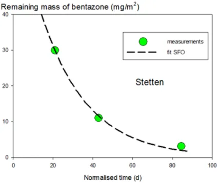
2.3.2.4 Field experiment at Stetten
The next field data set considered is Stetten (Hesse and Schepers 1991). Table 2-7 shows the calculated total amounts of bentazone and cumulative rainfall as a function of time and normalised time.
Table 2-7 Remaining amounts of bentazone in soil and cumulative rainfall as a function of time in the field experiment at Stetten.
Time
(d) Normalised time (d) Cumulative precipitation (mm) Areic mass (mg/m2) 0 0 0 75.7 7 4.48 3 53.0 13 9.41 3 32.0 29 20.98 16 29.9 61 42.87 111 11.0 103 84.51 168 3.1
The first step is to check whether SFO gives an acceptable fit based on normalised time and after eliminating data points before 10 mm of cumulative rain. Figure 2-10 shows that only three data points were left after this elimination and that the SFO fit to these points was visually acceptable. The χ2 error was 5% and the t-test of the rate coefficient was passed at a significance level of 4%. The resulting DegT50 of 16 d was considered acceptable in view of the good fit, although it was based on only three data points.
Page 30 of 96
Figure 2-10 Fit of the SFO model to the remaining amount of bentazone in the soil profile as a function of normalised time at Stetten. Points are measurements with cumulative rainfall above 10 mm and the line is the SFO fit.
2.3.2.5 Field experiment at Goch-Nierswalde
Table 2-8 shows the calculated total amounts and of bentazone cumulative rainfall as a function of time and normalised time for the field experiment Goch-Nierswalde.
Table 2-8 Remaining amounts of bentazone in soil and cumulative rainfall as a function of time in the field experiment at Goch-Nierswalde.
Time (d) Normalised time
(d) precipitation Cumulative (mm) Areic mass (mg/m2) 0 0 0 98.8 14 8.4 56 54.5 30 23.8 66 21.7 60 50.9 131 8.6 100 84.0 170 2.3
The first step is to check whether SFO gives an acceptable fit based on normalised time and after eliminating data points before 10 mm of cumulative rain. Figure 2-11 shows that only four data points were left and that the SFO fit to these points was visually acceptable.
Figure 2-11 Fit of the SFO model to the remaining amount of bentazone in the soil profile as a function of normalised time at Goch. Points are measurements with cumulative rainfall above 10 mm and the line is the SFO fit.
The χ2 error was 7% and the t-test of the rate coefficient was passed at a significance level of 0.9%. So the resulting DegT50 of 13 d was
considered acceptable.
2.3.2.6 Field experiment at Limburgerhof
Table 2-9 shows the calculated total amounts of bentazone and cumulative rainfall as a function of normalised time for the field
experiment at Limburgerhof. There was a complication with respect to the residues at day 14: in the layer at 37–50 cm depth a residue level of 0.06 mg/kg was measured, whereas the layers at 0–12 cm, 12–25 cm and 25–37 cm contained levels of 0.06, 0.04 and 0.03 mg/kg,
respectively. At day 30, residue levels of the 0–12 cm, 12–25 cm, 25–37 cm and 37–50 cm layers were <0.02, 0.02, 0.02 and <0.02 mg/kg, respectively. Schepers and Hesse (1991) considered the value of 0.06 mg/kg at day 14 in the 37–50 cm layer as a contamination because it is inconsistent with the other residue data. We agree because cumulative rain was 30 mm at day 14, so penetration of a significant fraction below 37 cm depth was unlikely. The texture of the soil is loamy sand (16% < 20 µm) so strong preferential flow effects are considered unlikely. Moreover, on day 30 the residue level in the 37–50 cm layer was less than that in the 25–37 cm layer. Therefore, the residue level in the 37– 50 cm layer on day 14 was set at <0.02 mg/kg.
Page 32 of 96
Table 2-9 Remaining amounts of bentazone in soil and cumulative rainfall as a function of time in the field experiment at Limburgerhof.
Time
(d) Normalised time (d) Cumulative precipitation (mm) Areic mass (mg/m2) 0 0 1 77.0 14 12.4 30 25.7 30 26.8 59 11.8 60 57.4 130 3.8
The first step is to check whether SFO gives an acceptable fit based on normalised time and after eliminating data points before 10 mm of cumulative rain. Figure 2-12 shows that only three data points were left and that the SFO fit to these points is visually acceptable.
Figure 2-12 Fit of the SFO model to the remaining amount of bentazone in the soil profile as a function of normalised time at Limburgerhof. Points are
measurements with cumulative rainfall above 10 mm and the line is the SFO fit.
The χ2 error was 5% and the t-test of the rate coefficient was passed at a significance level of 4%. So the resulting DegT50 of 17 d was
considered acceptable.
It should be noted that the rejection of the value of 0.06 mg/kg in the 37–50 cm layer after 14 d (normalised time 12.4 d) was in principle a conservative assumption: a higher value after 12.4 d normalised time would have decreased the estimated DegT50 because 14 d is the first data point in Figure 2-12. However, it is not certain that this is a conservative assumption because accepting the value of 0.06 mg/kg might have led to rejecting the SFO fit, thus leading to a bi-phasic fit with DFOP and possibly HS, which could have led to a higher estimated DegT50.
2.3.3 Combination of field and laboratory DegT50 values
EFSA (2014) gives a flow chart for the assessment of the DegT50
endpoint if DegT50 values from both field and laboratory experiments are available. The principle is that the laboratory DegT50 values can be rejected if it is demonstrated that the field DegT50 values are
significantly lower than the laboratory values. This has to be based on a statistical test with the null hypothesis that the geometric mean DegT50 of the laboratory experiments is equal to the geometric mean DegT50 of the field experiments. EFSA (2014) provides a calculator for performing this test. The significance level to be used is 25%.
We therefore have 27 laboratory DegT50 values with a geometric mean of 26 d and a standard deviation of the natural logarithms of 0.8, and four field DegT50 values of 13, 16, 17 and 19 d. The result of the test was that the geometric mean field DegT50 of 16 days is indeed significantly lower than the geometric mean laboratory DegT50. The significance level appeared to be between 12% and 13%. The flow chart of EFSA (2014) requires further that there be at least four field
DegT50 values. This requirement is fulfilled, so the DegT50 of 16 d is the endpoint of this DegT50 assessment, based on the EFSA flow chart. As described in Section 2.3.2.1, the field DegT50s have to be considered potentially unreliable because they were based on only 5–7 soil samples per sampling time. However, the four field DegT50s are in a narrow range (13–19 d), and it is considered unlikely that all four field studies resulted in too short a DegT50 because of the spatial variability in the measured soil residues: in total 13 soil samples (Havixbeck 3
(Figure 2-7), Stetten 3 (Figure 2-10), Goch-Nierswalde 4 (Figure 2-11) and Limburgerhof 3 (Figure 2-12) from different sampling times were used to fit these DegT50s. Therefore, the fact that there were only 5-7 sampling spots is not considered to be a problem.
EFSA (2010) collected a number of data sets of laboratory DegT50 measurements with the same substance and a range of soils and found that the standard deviation of the natural logarithms ranged between 0.2 and 0.5. So the value of 0.8 found here is considerably larger than the values found by EFSA (2010). However, the variation in the field DegT50s (normalised to 20 °C) is quite small (12–19 d): the standard deviation of the natural logarithms of 13, 16, 17 and 19 d is 0.16. EFSA (2010) reports two standard deviations of DegT50 values from field experiments: 0.4 and 0.6, i.e. considerably larger than for the field DegT50s of bentazone found here. A possible reason is the quite narrow pH range of the field soils considered (pHCaCl2 of 5.9 to 7.1). However, we could not find a correlation with pH in the laboratory studies as shown before.
Scorza Junior and Boesten (2005) performed a field experiment on a Dutch clay soil planted with winter wheat and obtained an inversely modelled field DegT50 of 12 d (using a measured Arrhenius activation energy of 74 kJ/mol). This value is close to the field DegT50 values reported here, but it is not included in the statistical test because it could not be evaluated in accordance with the EFSA (2014) guidance. The reason is that plant uptake may have played an important role in the dissipation of bentazone.
Page 34 of 96
There is a considerable safety margin in the rejection of the null
hypothesis: the actual significance level was 12–13% whereas a level of 25% is required. It is therefore considered unlikely that a further
detailed examination of the 27 other laboratory studies would have led to another conclusion of the DegT50 assessment.
2.4 Selected usages and assessment
Bentazone is applied to many crops. Two usage patterns were
evaluated: (A) usage typical of the period 1980–1990 and (B) current usage.
The selected usages were those expected to have the highest leaching. The usage typical of the period 1980–1990 was assumed to be an application of 1.44 kg/ha to maize on 25 May or the same rate in a series of crops on 15 October (PD 1991). Because the application date of 15 October results in higher leaching concentrations, the application to maize was ignored. On this basis, the usage covering the period
1980-1990 was defined as an application of 1.44 kg/ha to grass grown for seed generation on 15 October.
The highest leaching of bentazone can be expected from the highest dose and from application in autumn. The relevant current usage is application to grass (grown for seed generation) at a rate of 3 L/ha Basagran (i.e. 1.44 kg/ha bentazone). The usage label states that application should take place when the grass seedlings have three to five leaves and not later than 1 October. On this basis, the current usage was defined as an application of 1.44 kg/ha to grass grown for seed generation on 1 October. Calculations were also made for earlier application dates to check the effect of the application date.
In the stage of three to five leaves, the BBCH code used for grass is 10-19, based on the BBCH growth stages for cereals (Lancashire et al. 1991, Meier 2001). For this BBCH code a crop interception of 40% for grass (EFSA 2014) is used for the simulations.
The current approach is to subtract the amount intercepted from the application amount (FOCUS 2000), which implies that interception acts as a sink for the PPP. EFSA (2012) proposes accounting for the
dissipation of PPP from leaf surfaces and using 100 m-1 for the wash-off factor in combination with a half-life of 10 d for other dissipation
processes on the crop canopy, unless measured values are available. The proposed wash-off parameter may lead to a substantial increase in the amount of PPP estimated to reach the soil surface. It was therefore decided to do simulations for both the current approach and the
alternative proposed by EFSA. The latter approach is more conservative towards leaching.
The simulations were performed for both Tier 1 and Tier 2 of the decision tree for the usages indicated above. The physicochemical properties are given in Section 2.1 and the sorption and transformation data derived in Sections 2.2 and 2.3. As prescribed, the sorption
parameter for bentazone used in the Tier 1 calculations is the KOM,anion. All Tier 1 calculations, i.e. for the current method and the alternative
approach, assuming different crop canopy processes, led to
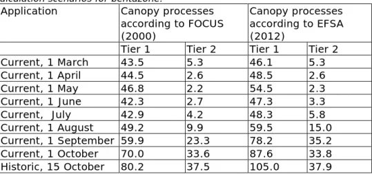
concentrations above the threshold limit. Therefore, Tier 2 assessments had to be performed. Table 2-10 shows the results of the calculations for eight application times in respect of current usage and one for the historic usage (application on 15 October), for both the two canopy parameterisations and the two tiers.
Table 2-10 90th-percentile leaching concentrations (µg/L) for different calculation scenarios for bentazone.
Application Canopy processes according to FOCUS (2000)
Canopy processes according to EFSA (2012)
Tier 1 Tier 2 Tier 1 Tier 2 Current, 1 March 43.5 5.3 46.1 5.3 Current, 1 April 44.5 2.6 48.5 2.6 Current, 1 May 46.8 2.2 54.5 2.3 Current, 1 June 42.3 2.7 47.3 3.3 Current, July 42.9 4.2 48.3 5.8 Current, 1 August 49.2 9.9 59.5 15.0 Current, 1 September 59.9 23.3 78.2 35.2 Current, 1 October 70.0 33.6 87.6 33.8 Historic, 15 October 80.2 37.5 105.0 37.9 All simulations result in 90th-percentile leaching concentrations of more than 20 times the acceptability level of 0.1 µg/L. The highest
concentration, 35.2 µg/L, is found for the September application with EFSA (2012) canopy parameters.
For the application timing giving the highest concentration (1 September), Figure 2-13 shows the cumulative frequency of the
calculated potential leaching concentrations after bentazone application of 1.44 kg/ha to grass with EFSA (2012) canopy parameterisation, and Figure 2-14 shows the geographical variability of leaching concentration. Figure 2-13 shows that the calculated concentration exceeds 0.1 µg/L for the whole area of use for this September application. Figure 2-14 shows that the highest concentrations are calculated for the clay areas in the northern and western parts of the Netherlands, and in the polders in the centre of the country.
The chosen historical application of bentazone results in a higher leaching concentration than the current 1 October application. This is due to the later timing of the application in the year, with higher net precipitation shortly after application.
Table 2-10 shows that setting the canopy parameters to the values recommended by EFSA (i.e. a DT50 of 10 days and a wash-off factor of 100 m-1) resulted in 90th-percentile concentrations that are similar to those using the FOCUS approach, which is remarkable. The crop
intercepts 40% of the loading, so with the FOCUS canopy approach 40% of the bentazone loading will not wash off to the soil, whereas with the EFSA canopy approach part of the 40% is expected to wash off to the soil. Hence, higher leaching concentrations would be expected from the EFSA approach. The application on 1 October leads to 90th-percentile
Page 36 of 96
concentrations of 33.6 µg/L (FOCUS) and 33.8 µg/L (EFSA). Such a small difference seems implausible with a crop interception of 40%. From the results of the simulations, the plot closest to the 90th
-percentile concentration was selected for further investigation. For the FOCUS canopy approach, this was plot 4918, where maize was used for the hydrology simulation (leaching concentration of 33.6 µg/L). For the EFSA canopy approach, it was plot 5386, where maize was also used for the hydrology simulation1 (leaching concentration 33.9 µg/L). For the EFSA approach the next closest plot to the 90th-percentile concentration was the same as the plot closest to the 90th-percentile in the FOCUS approach, i.e. plot 4918 (leaching concentration 33.6 µg/L). Hence, for plot 4918, where all other input is the same, the difference in approach has little effect on the leaching concentration. The mass balance of the canopies of plot 4918 revealed that almost all intercepted bentazone is removed with the harvest. The cropping period of maize is 20 May to 17 October.
Figure 2-13 Potential leaching concentrations after bentazone application of 1.44 kg/ha on 1 September, with wash-off from leaves (EFSA parameterisation of canopy processes)
1 GeoPEARL simulates the hydrology of a plot using crop parameters of the crop representing dominant land use in the plot. Furthermore, each crop is assigned to one of four land uses: grass, maize, potatoes or nature.
Figure 2-14 Map of bentazone leaching concentrations (50th percentiles) after application of 1.44 kg/ha on 1 September to grass, with wash-off from leaves (EFSA canopy parameterisation)
If all bentazone on the crop canopy washes off, concentrations can be a factor 100%/(100%–40%) higher in the EFSA approach than in the FOCUS approach. Only the August and September applications show higher leaching concentrations with the EFSA approach than with the FOCUS approach. The leaching concentrations from other application timings in the cropping period hardly differ for the two approaches. Hence, the new EFSA canopy parameterisation may not fit with how crops are simulated in GeoPEARL.
Page 38 of 96
The 90th-percentile concentration of bentazone in groundwater exceeds the drinking water limit of 0.1 µg/L calculated by GeoPEARL for the worst case crop (with respect to leaching), which is grass grown for seed production, using the improved guidance proposed by Boesten et al. (2015) for the determination of sorption and transformation parameter values of bentazone with studies available in the dossier and in
3
MCPA
3.1 General information on MCPA
This section provides general information on and the physicochemical characteristics of MCPA (see also Table 3-1) according to the List of Endpoints (LoEP) on MCPA (EC 2008).
Table 3-1 Physicochemical properties of MCPA (EC 2008).
Active substance (ISO
common name) MCPA
Chemical name (IUPAC) 4-chloro-o-tolyloxyacetic acid Molecular formula C9H9Cl03 Molecular mass 200.6 Structural formula Vapour pressure (Vp) 4 x 10⁻⁴ Pa at 32 °C (99.4%) 4 x 10⁻³ Pa at 45 °C (99.4%)
Solubility in water Solution Solubility (g/L) at 25 °C pH=1 unbuffered 0.395 ± 9.1
pH=5 buffered 26.216 ± 1.403 pH=7 buffered 293.898 ± 5.329 pH=9 buffered 320.093 ± 5.945 Purity = 99.4 %
Hydrolytic stability (DT50) 14C-MCPA acid was stable to hydrolytic degradation at pH 5, 7 and 9 at 25 °C for 30 days.
Dissociation constant pKa = 3.73 (s = 0.07) at 20 °C pKa = 3.73 (s = 0.00) at 25 °C Purity = 99.8 %
MCPA is slightly volatile and its water solubility is very high for its salts.
3.2 Sorption
A scan of the MCPA dossier and published literature (not an in-depth literature search) revealed a high number of sorption studies. Only studies with unaltered soils, i.e. soils without added material (e.g. peat and ash) that could influence the sorption of MCPA, were taken into consideration. An overview of the studies, with the (not-corrected) sorption constants, is given in Figure 3-1 and the individual values are given in Appendix B. In total, 134 sorption experiments (115 batch values, 14 column values and 5 soil TLC values) were examined. Details on the handling of MCPA column leaching and soil TLC studies are also given in Appendix B.
OCH
2COOH
CH
3Cl
Page 40 of 96
Figure 3-1 Overview of raw sorption data of MCPA. Reported pH values are converted to pHKCl where appropriate, assuming pHH2O when not reported. KOM values are not corrected.
MCPA is a substance whose dissociation status depends on the pH of the soil. As the pKa of MCPA is 3.73, it is expected that its sorption is also dependent upon the pH of the soil. Sorption constants and pH values are used to derive a sorption curve. In this case, both pH values and
sorption constants have to be sufficiently reliable. Studies were assessed for completeness of information and quality of the experiments in order to derive reliable sorption constants and the most appropriate function for the dependency of the sorption on the pH of the soil. pHKCl was chosen to construct the relationship, in line with the soil pH map contained in GeoPEARL.
The selection of reliable values followed a stepped approach. Table B-3 in Appendix B gives the selection step at which values were considered not sufficiently reliable or not fulfilling the requirements of the
authorisation assessment procedure. This selection elaborates on the procedure described in section 3.6.3 (step 1) of Boesten et al. (2011).
(http://www.rivm.nl/bibliotheek/rapporten/2015-0095MCPA_sorption_data.xlsm)
3.2.1 Selection of MCPA sorption coefficients
Step 1: elimination of duplicates and data with insufficient quality In this step ‘insufficient quality’ is assigned to data with:
• a missing pH value
• a missing sorption constant (KD, KF, KOC, KOM), or a sorption constant given as a maximum
• an incorrect or uncertain calculation method where the basic experimental data is not available (if basic data was available, the sorption data were recalculated)
• an unknown water layer in column studies • an unknown water flow rate in column studies • an unknown penetration depth or column length.
Where duplicates (different values reported for the same soil) remained after applying the quality criteria, expert judgement was applied to select the most reliable values. In the three cases where duplicate values remained, the values according to the batch equilibrium method were preferred because the description of the experiments was
considered to be more complete.
After this step, 100 values remained: 97 batch, 1 column and 2 TLC values.
Step 2: removal of data with suspected influence of transformation When the indirect batch equilibrium method is used, prolonged
equilibration time may lead to excessively high sorption values because of transformation. According to the indirect method, the difference between the initial and equilibrium concentrations is the basis for the calculation of the sorption. If the transformation is higher than the default limit (10%), the proposed correction based on the minimum recovery of 90% (see Boesten et al. (2011)) may be insufficient. All data obtained in experiments without any sterilisation and an equilibration time of four days or longer was considered to have insufficient quality at this step.
After this step, 60 values remained, including 1 column and 2 TLC values.
Step 3: removal of sediments and soils from below the plough layer Standard evaluation/assessment considers topsoils only, so values for sediments and subsoils (i.e. soils deeper than 30 cm) were removed from the selection.
After this step, 42 values remained, including 1 column and 2 TLC values.
Step 4: removal of data from soils with low organic matter/organic carbon content.
In soils with low organic matter, sorption onto other surfaces may contribute significantly to the overall observed sorption. It has become common practice not to include sorption constants from soils with low organic matter content (%OM < 0.5, %OC < 0.3) in the calculation of the average sorption constant. Sorption values fulfilling this criterion were removed. The limit values are taken (or derived) from Mensink et al. (2008).
After this step, 40 values remained, including 1 column and 2 TLC values.
OECD106 prescribes not using the indirect method for determining the sorption constant when the decline in concentration in the liquid phase is less than 20%. In nearly 60% (22 out of 37) of the batch experiments remaining after the fourth selection step, the decline in concentration in the liquid phase was less than 20%. It was, however, decided not to use
Page 42 of 96
this as a deselection criterion, as many of the experiments were performed before the guideline was published in 2000.
Figure 3-2 gives an overview of the data remaining after the selection procedure as well as the data deselected at the various steps (except data deselected in step 1, as this data was not considered reliable enough for this study).
Figure 3-2 Corrected KOM versus pHKCl. Selection 2 – 4 indicate the data points deselected in step 2 – 4 of the selection procedure. pH unknown indicates the points for which the pH measurement method was not stated. The series pH known, pH unknown, TLC and column remained after step 4 of the selection procedure.
All KOM values remaining after the fourth step (see Appendix B) were considered to be reliable enough and belonging to the correct population of sorption values to be used for deriving the function relating the
sorption of MCPA to soil pH. However, for 16 experiments the pH measurement method was not stated in the available information. So, for these data points there is uncertainty about the pH. The default when the measurement method is missing is to assume that the measurement method is according to pHH2O, which is conservative because the correction will shift points to the left when figures are converted to pHKCl or pHCaCl2 for practically all relevant pH values. The uncertainty in the pH was nevertheless investigated further (see below). Figure 3-3 gives reported as well as corrected KOM values for the data points remaining after step 4. Because of the number of values remaining after the selection procedure, the graphs presented here deviate from the recommended graphs; a graph with all connection lines between uncorrected and corrected points for both KOM and pH would be illegible. For data with a known pH measurement method, only the correction for KOM is given. (Note that the correction procedure leads to