National Institute for Public Health and the Environment
P.O. Box 1 | 3720 BA Bilthoven www.rivm.com
Model-Then-Add
Usual intake modelling of multimodal intake distributions
RIVM Letter report 090133001/2014 H. van der Voet et al.
Colophon
© RIVM, DLO 2014
Parts of this publication may be reproduced, provided acknowledgement is given to: National Institute for Public Health and the Environment and Wageningen University and Research centre, along with the title and year of publication.
Hilko van der Voet* Johannes Kruisselbrink* Waldo J de Boer* Polly E. Boon
* Biometris, DLO, Wageningen University and Research centre
Contact: Polly E. Boon
Centre for Nutrition, Prevention and Health Services, Food Safety polly.boon@rivm.nl
This investigation has been performed by order and for the account of
Netherlands Food and Consumer Product Safety Authority (NVWA), Office of Risk Assessment, within the framework of Project ‘Modelling exposure contaminants', research question 9.1.33
Rapport in het kort
Model-Then-Add
Berekening van de gebruikelijke inname bij multimodale innameverdelingen
Het RIVM heeft met de Wageningen Universiteit (WUR) software ontwikkeld waarmee kan worden berekend hoeveel chemische stoffen mensen
binnenkrijgen via de voeding (Monte Carlo Risk Assessment; MCRA). Enkele voorbeelden van zulke stoffen zijn contaminanten (acrylamide, dioxine, lood) en micronutriënten. Om de inname op de lange termijn te kunnen berekenen, is een module aan deze software toegevoegd, Model-Then-Add. De lange termijn inname is relevant bij chemische stoffen die niet meteen maar pas na verloop van tijd een gunstig of schadelijk effect op de gezondheid kunnen veroorzaken. De Model-Then-Add-module kan worden gebruikt als de gemiddelde
innameverdeling bij een groep mensen statistisch gezien geen ‘normale’ curve vertoont, bijvoorbeeld als de stof maar in een beperkt aantal producten voorkomt. De module kan in dergelijke gevallen een realistischere inschatting van de lange termijn inname geven.
Voor dit onderzoek is een case-study uitgewerkt naar de lange termijn inname van rookaroma’s, een potentieel schadelijke groep stoffen bij hogere innamen. De inname is berekend met de Model-Then-Add-module en de huidige
methodiek, waarvan bekend is dat het de lange-termijn inname overschat. Hieruit blijkt dat de inname van rookaroma’s volgens de Model-Then-Add-module lager is. Door dergelijke nauwkeurigere, lagere innamen van schadelijke stoffen zijn mogelijk minder (kostbare) maatregelen nodig om
gezondheidsrisico’s te verlagen, zoals lagere normen voor concentraties in producten.
Om de inname van chemische stoffen via de voeding met MCRA te berekenen, worden concentraties van stoffen in de voeding gekoppeld aan gegevens over wat mensen gedurende enkele dagen consumeren. In Nederland zijn dat de gegevens van de Voedselconsumptiepeiling (VCP), waarin informatie over de consumptie van voedingsmiddelen gedurende twee dagen wordt verzameld. Statistische modellen zijn nodig om op basis van deze gegevens in te schatten hoeveel van de chemische stoffen mensen op termijn via de voeding
binnenkrijgen.
Trefwoorden:
Abstract
Model-Then-Add
Usual intake modelling of multimodal intake distributions
The National Institute for Public Health and the Environment (RIVM) and Wageningen University and Research Centre (WUR) have jointly developed software to estimate the amount of chemicals ingested via the diet (Monte Carlo Risk Assessment, MCRA). Examples of such chemicals include contaminants (e.g. acrylamide, dioxins, lead) and micronutrients. To estimate the intake of these chemicals in the long run, a module called Model-Then-Add has been added to the software. The long-term intake is relevant for chemicals that exert their beneficial or adverse health effect over a long period of ingestion. The Model-Then-Add module can be used when the distribution of individual mean intakes of the chemical in a population does not display a normal statistical distribution after a logarithmic transformation. This may, for example, be the case when the chemical is present in only a limited number of foods. In such cases, the module can be used to obtain a more realistic estimation of the long-term intake.
A case study was performed to assess the long-term intake of smoke aromas, a group of chemicals that is potentially adverse at high intakes, using the Model-Then-Add module and the presently used methodology, which is known to overestimate the long-term exposure. The Model-Then-Add module resulted in lower intakes. The use of this module may thus result in less risk mitigation or environmental policy measures that need to be taken to reduce possible health risks.
To estimate the intake of chemicals via the diet using MCRA, concentrations of chemicals in foods and beverages are linked to information on the consumption of these foods during a limited number of days. In the Netherlands, food consumption data are typically obtained from the Dutch National Food
Consumption Surveys (Voedselconsumptiepeiling, VCP), in which information on food consumption is collected during two days. Statistical models are necessary to assess the long-term intake of chemicals based on these data.
Keywords:
Content
1
Introduction—6
2
Methodology—7
3
Case study: smoke flavours—10
3.1
Introduction—10
3.2
Results—10
3.2.1
Young children—10 3.2.2
Adults—10
4
Discussion and recommendations—14
Acknowledgements—17
References—18
Appendix I. Concentration data of smoke flavours—20
Appendix II. Consumption of foods containing smoke flavours—21
Appendix III. OIM exposure distributions to smoke flavours for the 17 individual foods-as-measured (alphabetical order) in young children—23
1
Introduction
To assess the long-term dietary intake of (or exposure to) chemical substances, both beneficial and adverse, statistical models may be used in higher tier assessments to estimate the long-term intake corrected for the within-person variation (Hoffmann et al., 2002; Nusser et al., 1996; Slob, 1993). Long-term intake is also termed usual or habitual intake. These two terms will be used interchangeably in this report. Examples of models for usual intake are the betabinomial-normal (BBN) and the lognormal-normal (LNN) model, which are both implemented in the Monte Carlo Risk Assessment (MCRA) program (de Boer and van der Voet, 2011). Both models are based on the principle of separately modelling intake frequencies and intake amounts, followed by an integration step. In both BBN and LNN, intake amounts, after a logarithmic or power transformation, are assumed to be normally distributed. In MCRA, this assumption can be checked by using the normal quantile–quantile (q–q) plot, a graphical display of residuals (de Boer et al., 2009). If the criterion of normality is severely violated, use of models like BBN and LNN may result in erroneous intake estimates that are either too high or too low.
In those cases, the Observed Individual Mean (OIM) method is presently the commonly used alternative method available within MCRA. This method calculates the mean intake over the survey days present in the food
consumption database per individual as a proxy for long-term intake (see e.g. Dodd et al., 2006). This approach is not dependent on model assumptions, but is known to overestimate the intake in the upper tail of the intake distribution (Boon et al., 2011; Boon et al., 2012; Goedhart et al., 2012).
Non-normality is a commonly found phenomenon when long-term intake is considered. The development of the Model-Then-Add method within MCRA, as an approach to address this, started when assessing the long-term exposure to patulin, which was found to be multimodal due to the contributions of multiple distinct foods to the exposure (de Boer et al., 2009). A simulation model, available in MCRA 7.1 (de Boer and van der Voet, 2011) made it possible to visualise the multimodal distributions that can arise from exposure via multiple foods. Based on these and similar experiences the Model-Then-Add approach was conceived, and a simple case was tested in a simulation study, with positive results (Slob et al., 2010). In this study, the exposure per food or groups of foods was modelled separately using BBN, and then estimates per food or food group were added to estimate the overall exposure distribution. In a recent simulation study, it was concluded that in cases of non-normality a Model-Then-Add approach could be helpful (Goedhart et al., 2012). In the field of nutrition, a comparable approach has been developed to address the total intake of
nutrients via the diet and other sources like food supplements (van Rossum et al., 2012; van Rossum et al., 2011; Verkaik-Kloosterman et al., 2012; Verkaik-Kloosterman et al., 2011).
In the research project described in this letter report, a Model-Then-Add approach was fully developed and implemented in MCRA version 8.01
(MCRA, 2013). To demonstrate how the approach works, we assessed the exposure to smoke flavours, a potentially adverse group of chemicals at high intakes, using OIM and the Model-Then-Add approach.
2
Methodology
Long-term dietary intake assessments usually proceed by first calculating the intake per food for each person-day (e.g. intake to chemical X per person-day via apple, intake to chemical X per person-day via pear, etc.). These intakes are then summed over the foods (intake to chemical X per person-day) to calculate the total intake per day, and finally to estimate the usual intake (intake to chemical X per person, averaged over days) by applying a statistical model to the person-day intakes. To apply these models (including MCRA’s BBN and LNN models), the person-day intake distribution should be approximately normally distributed after a suitable transformation. This traditional approach can also be termed the Add-Then-Model approach, because adding over foods precedes the statistical modelling.
An alternative approach developed in this research is Model-Then-Add2. In this
approach the statistical model is applied to subsets of the diet (single foods or food groups), and then the resulting usual intake distributions per food or food group are added to obtain an overall usual intake distribution. The advantage of this approach is that the intake via separate foods or food groups may show a better fit to a normal distribution than via all foods together. The concept was tested and shown to work in previous studies (de Boer et al., 2009, Slob et al., 2010, Goedhart et al., 2012). A practical approach to apply Model-Then-Add within MCRA was however still missing. Therefore, a module in MCRA 8.0 was developed to make this approach available for usual intake modelling. Below we describe the principles behind the Model-Then-Add approach as implemented in MCRA using the example of dietary exposure to smoke flavours in young children (see section 3 for more details).
The Model step
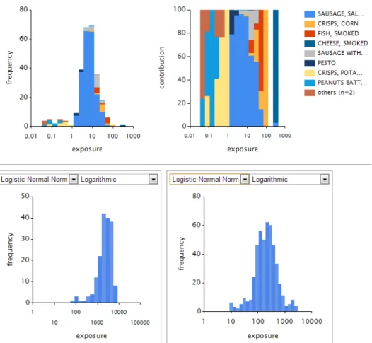
The Model step starts with a separation of individual foods or food groups from the total intake distribution. At this stage of model development, this separation is performed in an interactive process, where the MCRA user is presented with a visual display (see example in Figure 1), which shows:
1. The OIM intake distribution represented as a histogram, where each bar shows the frequency of intakes (summed over foods) of individuals in a certain intake interval. Each bar is subdivided according to the contributions of the individual foods contributing to those intakes (left panel of Figure 1). 2. The contributions graph, where each of the bars in the OIM intake
histogram is expanded to 100%. This graph allows a better view of the lower bars in the OIM intake histogram (right panel of Figure 1). The visual display identifies the nine foods that contribute most to the total intake. The remaining foods are grouped in a rest category to avoid
identification problems because of too many colours.
The user has now the possibility to select one food or food group and to separate it from the main intake histogram. A separate graph shows the OIM intake distribution for this food or food group. The graphs for the main group (now called the rest group) are adapted to show the OIM intake distribution and the contributions for the remaining foods (upper two panels of Figure 2).
2 The terminology of Add-Then-Model and Model-Then-Add is similar to the terminology of Add, then Shrink vs.
Shrink, then Add, as introduced by Kevin Dodd during various presentations. We prefer our terminology because modelling has more aspects than only the shrinking towards the mean (e.g. the type of transformation chosen).
This separation of foods or food groups from the main intake histogram can be repeated several times. In this way, the user can try to obtain foods or food groups that show unimodal OIM intake distributions that can be modelled using LNN or BNN. In an iterative process, a food or food group can be added
Figure 1. Left panel: OIM exposure distribution to smoke flavours via the different foods (excluding the zero exposures) in young children; Right panel: contribution of foods to exposures within each bar of the OIM distribution histogram.
Figure 2. Result of a selection into two separate food groups and a rest group. The graph bottom left represents the exposure via a food group containing ‘Sausage, frankfurter’ and ‘Sausage, smoked cooked’. The graph bottom right represents the exposure via a food group containing ‘Sausage, luncheon meat’, ‘Herbs, mixed, main brands, not prepared’, ‘Soup, pea’, ‘Ham’, and ‘Bacon’. The top graph represents the exposure via the rest group.
again or separated from the rest group until a satisfactorily result is obtained. Per separate food or food group the usual intake can be modelled using BBN or LNN, with a logarithmic or power transformation. The rest group, containing foods for which no unimodal OIM intake distributions can be obtained, will be modelled using OIM. It is possible that the rest group is empty, when the total intake via the different foods and /or food groups can be modelled with BBN or LNN.
After the separation of food or food groups is finalised, the OIM intake
distribution is summarised in terms of the defined grouping (Figure 3), and the usual intake distribution per food or food group is fitted according to the chosen modelling settings.
The Add step
In this step, the estimated usual intake distributions per food or food group are combined to assess the total usual intake. The combination can be made in several ways. In this report we describe only the simplest option. For this, the intake distributions per food or food group, including the rest group if present, are sampled independently (where the number of Monte Carlo iterations can be chosen in MCRA) and subsequently added to obtain the overall usual intake distribution (model-based approach3)4. In this approach, correlations in the
consumption of foods are not addressed as in the traditional Add-Then-Model approach where the Add step automatically reflects any correlations that are apparent in the consumptions at the individual-day or individual level. Performing the Add step without considering possible correlations in food consumption was investigated by Slob et al. (2010) and performed surprisingly well, even if correlations in consumptions of foods were present.
3 An alternative ‘model-assisted’ approach allowing for correlations, is also available, and is described in the
Reference Manual (MCRA 2013). Also see the Discussion section.
4 Before the addition is made, the usual exposure estimates per food or food group modelled with BNN or LNN
are back-transformed, and the frequency distribution is sampled to decide if a simulated individual has exposure via the food or food group or not.
Figure 3. OIM exposure distribution showing the contributions from the three food groups as constructed in Figure 2.
3
Case study: smoke flavours
3.1 Introduction
To show the potential of the Model-Then-Add approach, we performed a case study on the exposure to smoke flavours using the concentration and food consumption data used by Sprong (2013). In this study, the long-term exposure to smoke flavours was estimated in three different age groups in the
Netherlands: young children (2-6 years), children (7-18 years) and adults (19-69 years). The assessment was performed using the OIM approach (Sprong, 2013). A statistical model to assess the usual intake was not used by Sprong (2013), because the transformed daily exposure data did not meet the normality criterion in any of the age groups (de Boer et al., 2009). We used these data to show the possibilities of the Model-Then-Add approach to refine the exposure assessment for young children (2-6 years) and adults (19-69 years) as opposed to the OIM model. The age group children (7-18 years) was not addressed. See Appendix I for an overview of the concentration data used and Appendix II for the corresponding food consumption data for both age groups.
3.2 Results
3.2.1 Young children
The dietary exposure to smoke flavours using the OIM model was trimodal (Figure 1, left panel). The use of BBN or LNN to assess the usual exposure to smoke flavours was therefore not feasible as concluded by Sprong (2013). As a first test, we calculated OIM exposure distributions for all 17 foods individually (Appendix III). For many foods the number of positive exposure values was very limited. Grouping of foods had to be made for a meaningful parametric
modelling.
Visual inspection of the joint OIM exposure distribution (Figure 1) and a comparison of the individual distributions (Appendix III) showed that the exposure in the upper part of the log-transformed exposure distribution in children was mainly due to the consumption of ‘Sausage, frankfurter ‘, ‘Sausage, smoked cooked’, and ‘Soup, pea’. We labelled these foods as the Top3 food group. The middle peak in the exposure distribution seemed mainly to be connected with the consumption of ‘Bacon, ‘Ham, ‘Herbs, mixed, main brands, not prepared’, and ‘Sausage, luncheon meat’. We labelled these foods as the Mid4 food group. The foods in the Top3 and Mid4 food groups explained most (80%) of the total exposure to smoke flavours (Figure 4). Therefore, the remaining foods were left in the rest group to be modelled with OIM.
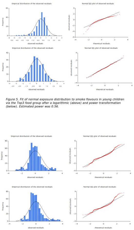
Several models were fitted to assess the long-term exposure (Table 1). Some of the diagnostic plots are shown in Figure 5 and 6. Compared to the OIM exposure results, high percentiles of exposure were much lower when the exposure via the Top3 food group was modelled separately from the remainder of the foods (with or without the Mid4 food group). Modelling the exposure separately per food (AllSep) did only result in a slight reduction in exposure estimates in the upper tail of the exposure distribution compared to OIM. A power transformation improved the fit of the Top3 food group (but not the Mid4 food group) (Figures 5 and 6), and led to lower percentiles at the tail of the distribution (Table 1).
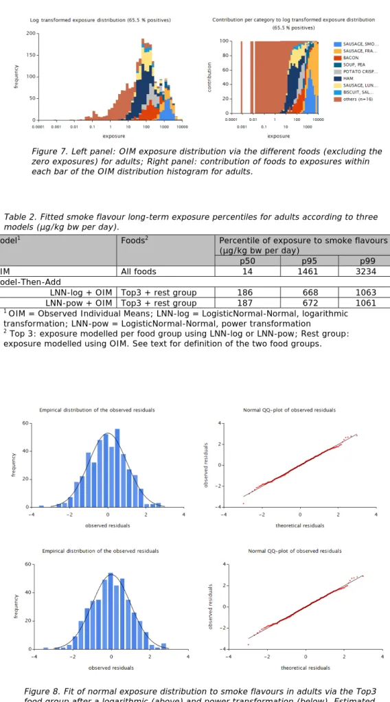
3.2.2 Adults
For adults, the OIM exposure distribution was also trimodal (Figure 7). As for young children, foods contributing most to the upper tail of the OIM exposure
distribution were ‘Sausage, smoked cooked’, ‘Sausage, frankfurter’, and ‘Soup, pea’. These three foods were merged in a Top3 food group. The remainder of the foods were kept in the rest group. We restricted the exposure assessment for the adults to this scenario.
The exposure to smoke flavours was estimated using different models, as done in young children (section 3.2.1). The results are presented in Table 2. Figure 8 shows the diagnostic plots for the Top3 exposure distribution for both
transformations (logarithmic and power). The high percentiles of exposure were much lower when the Model-Then–Add approach was used (Table 2). A power transformation resulted in the same outcome as a logarithmic transformation: the estimated power was close to zero (Figure 8).
Table 1. Fitted smoke flavour long-term exposure percentiles for young children (2-6 years) according to several models (µg/kg bw per day).
Model1 Foods1 Percentile of exposure to smoke flavours
(µg/kg bw per day)
p50 p95 p99
OIM All foods 7 3307 5498
Model-Then-Add
LNN-log + OIM Top3 + rest group 459 1247 1899
LNN-pow + OIM Top3 + rest group 457 1040 1503
LNN-log +OIM Top3 + Mid4 + rest group 531 1206 1747
LNN-pow + OIM Top3 + Mid4 + rest group 534 970 1233
LNN-log AllSep 644 1768 4757
LNN-pow AllSep 642 1554 4634
1 OIM = Observed Individual Means; LNN-log = LogisticNormal-Normal, logarithmic
transformation; LNN-pow = LogisticNormal-Normal, power transformation
2 Top 3 and Mid4: exposure modelled per food group using LNN-log or LNN-pow; Rest
group: exposure modelled using OIM; AllSep = exposure modelled separately per food using LNN-log or LNN-pow and then added. See text for definition of the three food groups.
Figure 4. Contribution of the individual foods to total exposure to smoke flavours in young children.
Figure 5. Fit of normal exposure distribution to smoke flavours in young children via the Top3 food group after a logarithmic (above) and power transformation (below). Estimated power was 0.56.
Figure 6. Fit of normal exposure distribution to smoke flavours in young children via the Mid4 food group after a logarithmic (above) and power transformation (below). Estimated power was 0.14.
Table 2. Fitted smoke flavour long-term exposure percentiles for adults according to three models (µg/kg bw per day).
Model1 Foods2 Percentile of exposure to smoke flavours
(µg/kg bw per day)
p50 p95 p99
OIM All foods 14 1461 3234
Model-Then-Add
LNN-log + OIM Top3 + rest group 186 668 1063
LNN-pow + OIM Top3 + rest group 187 672 1061
1 OIM = Observed Individual Means; LNN-log = LogisticNormal-Normal, logarithmic
transformation; LNN-pow = LogisticNormal-Normal, power transformation
2 Top 3: exposure modelled per food group using LNN-log or LNN-pow; Rest group:
exposure modelled using OIM. See text for definition of the two food groups.
Figure 8. Fit of normal exposure distribution to smoke flavours in adults via the Top3 food group after a logarithmic (above) and power transformation (below). Estimated power was 0.02.
Figure 7. Left panel: OIM exposure distribution via the different foods (excluding the zero exposures) for adults; Right panel: contribution of foods to exposures within each bar of the OIM distribution histogram for adults.
4
Discussion and recommendations
In this report, we showed that the Model-Then-Add approach resulted in lower estimates of exposure in the upper part of the long-term exposure distribution compared to the Observed Individual Mean (OIM) approach.
OIM vs. Model-Then-Add
The OIM approach to assess the usual intake is a simple methodology to assess the long-term intake to chemical substances present in food. This methodology is presently used by the European Food Safety Authority (EFSA) to assess the long-term exposure to contaminants (e.g. EFSA, 2012a, c; 2013). However, it is generally known that this approach results in conservative estimates of the upper percentiles of the usual exposure distribution (Boon et al., 2011; Boon et al., 2012; Goedhart et al., 2012). To refine the usual exposure assessment, statistical models such as the lognormal-normal (LNN) or betabinomial-normal (BNN) models as implemented in MCRA (de Boer and van der Voet, 2011) can be used by removing the within-person (between days) variation from the daily exposure distribution. An important prerequisite for this is however that the daily exposure distribution is normally distributed after a suitable transformation (de Boer et al., 2009). This criterion cannot be met when the daily exposure distribution is multimodal. To date, only the OIM approach within MCRA could be used in this situation.
In this research project, we implemented in MCRA an alternative for OIM, namely the Model-Then-Add approach, to assess the usual intake in cases of multimodality (Goedhart et al., 2012). We demonstrated that this approach can be applied in these cases and that this can result in lower, more refined upper tail percentiles of exposure compared to the OIM exposure estimates. The Model-Then-Add approach consist of carefully creating food groups or selecting foods with unimodal OIM exposure distributions, and modelling the exposure per food or food group using LNN or BBN (and OIM for the rest group) before adding the exposures to obtain the total usual exposure distribution. A strategy where all foods were modelled separately using LNN was not successful and led again to high percentiles of usual exposure (Table 1), due to the limited exposure data for a number of individual foods (Appendix III).
Use of Model-Then-Add approach to assess the exposure to smoke flavours
To illustrate the use of the Model-Then-Add approach, we assessed the exposure to smoke flavours using data from Sprong (2013). In that study, OIM was used to assess the long-term exposure because the daily exposure distributions were multimodal. We assessed the exposure in young children (2-6 years) and adults (19-69 years) using OIM and the Model-Then-Add approach.
In both adults and young children, a Top3 food group was identified for separate modelling of exposure using LNN. The exposure via the remainder of the foods was modelled using OIM. In young children, the OIM exposure distribution via this Top3 food group still had a non-symmetric distribution (Figure 5). However, the distribution was unimodal, and therefore a power transformation could be used to obtain a good fit (Figure 5). The P99 of exposure obtained in this manner was a factor 3.7 lower than the OIM P99: 1503 vs. 5498 µg/kg bw per day (Table 1). In adults, the exposure via the Top3 food group performed a good fit for both types of transformations (Figure 8). The Model-Then-Add P99 of exposure to smoke flavours in this population was more than halved
In the young children, also a Mid4 food group was identified for possible
separate modelling of exposure using LNN. The OIM exposure distribution of this food group showed still some multimodality, and in this case a transformation did not help to achieve normality (Figure 6). Given that the major contributions to the total exposure to smoke flavours came from the Top3 food group
(Figure 4), it may be acceptable to leave all other foods in the rest group to be modelled via OIM. For this age group, the Top3 LNN, power transformation model represented therefore the method of choice among the investigated models to assess the usual exposure to smoke flavours.
The Add step: model-based vs. model-assisted
In the Add step of the Model-Then-Add approach the modelled exposures per food or food group (including the rest group, if relevant) are added to obtain a total exposure intake distribution. In the approach applied here, the exposures were added using a model-based approach. In this approach, exposures per food or food group are independently sampled from the separate exposure distributions and subsequently added to obtain the total usual exposure distribution. This approach ignores possible positive or negative correlations between the foods consumed, and may result respectively in either an under- or overestimation of the intake. Slob et al (2010) showed an example where performing the Add step without considering possible correlations in food consumption performed well, even if correlations in consumptions of foods were present. More research is needed to establish how robust this result is.
In MCRA, an approach is available to take correlations between the consumption of foods into account in the Add step, the so-called model-assisted approach (van Klaveren et al., 2012, Goedhart et al., 2012)5. Goedhart et al. (2012)
concluded that in the traditional Add-Then-Model approach the model-assisted percentiles appear to be more robust to departures from normality for the positive amounts than the model-based percentiles.
Use of the Model-Then-Add approach
The Model-Then-Add approach is an alternative to the OIM approach in cases of multimodality, and if a unimodal OIM intake distribution can be defined for one or more foods or food groups that can be modelled. In food safety the interest lies with the upper tail of the intake distribution. To refine an intake estimate using Model-Then-Add as opposed to OIM preferably foods or food groups need to be defined that contribute to the upper tail of the intake distribution, as was done in the case study on smoke flavours (Top3).
Multimodality can arise when the intake to a chemical substance occurs via the consumption of a limited number of foods, like smoke flavours or other food additives that are not omnipresent in foods (like dioxins or lead). Another example in which the Model-Then-Add approach may be useful to assess the long-term exposure is when the exposure to a chemical substance via one food is significantly higher than via the rest of the diet, due to high concentrations in that food. An example of this is the setting of maximum residue levels for pesticides that are already allowed on the market using a probabilistic approach (EFSA, 2012b). In that case, the usual exposure to the relevant pesticide should be calculated by using residue levels from supervised trials in the commodity of relevance (focal commodity) and monitoring data in all other commodities in which residues of the pesticide may be present (background commodities).
5 Model-assisted estimates of the usual exposure distribution are back-transformed values from a shrunken
version of the transformed OIM distribution, also done per food or food group, where the shrinkage factor is based on the variance components estimated using the linear mixed model for amounts at the transformed scale. For individuals with no observed exposure (OIM=0) no model-assisted estimate of usual exposure can be made and a model-based replacement is used.
Since concentrations found in monitoring are often much lower than the concentrations analysed in field trial studies, the use of these two types of concentration data will very likely result in a bimodal exposure distribution. By modelling the exposure via the focal commodity separately from the exposure via the background commodities, the Model-Then-Add approach can result in a more refined exposure assessment compared to OIM, as is presently
recommended (EFSA, 2012b).
Recommendations
The case study addressing the exposure to smoke flavours has given a first example of the Model-Then-Add approach. More research is needed on how the approach would perform in other case studies, including the use of the model-assisted approach to add the exposures per food or food group. It is also relevant to consider whether the formation of relevant food groups can be automated.
Another issue is that sometimes it may be better to construct food groups based on foods-as-eaten instead of foods-as-measured. In the case study,
concentration data on smoke flavours were available in foods-as-eaten. However, in, for example, exposure assessments to contaminants or pesticide residues, these two are often not the same: chemical substances may be measured on raw agricultural commodities that are ingredients of foods-as-eaten. It is an open question for further research if the separation of foods or food groups can be performed best at the level of eaten or foods-as-measured.
Furthermore, the present implementation of the Model-Then-Add approach does not allow covariate modelling of exposure. It is however known that, for
example, young children and elderly or men vs. women have different consumption patterns that may result in deviations from normality. Covariate modelling, which is also available in MCRA, is thus a further possibility for parametric modelling. How this should be used exactly in combination with the Model-Then-Add approach remains to be investigated.
Finally, we tested the model using an example within the field of food safety. This model can however also be applied within the field of nutrition, e.g. when assessing usual total nutrient intake via the diet and dietary supplements. An example of this can be found in Verkaik-Kloosterman et al. (2011).
Conclusion
The Model-Then-Add approach as implemented in MCRA is a welcome addition to the models for usual exposure, and can provide more realistic estimates of higher exposures when the assumption of a normal distribution for the positive exposures after a suitable transformation is not met. Using this approach as opposed to the more conservative OIM approach in such cases may result in lower exposures and thus in less risk mitigation or environmental policy measures that need to be taken to reduce possible health risks.
Acknowledgements
The authors would like to thank Jeljer Hoekstra, Arnold Dekkers and Corinne Sprong of the RIVM for their valuable contribution to an almost finalised version of the letter report. The Federation of the Dutch Food and Grocery Industry (FNLI) is kindly acknowledged for allowing us to use the concentration data on smoke flavours to illustrate the Model-Then-Add approach.
References
Boon, P.E., Bonthuis, M., van der Voet, H., van Klaveren, J.D., 2011.
Comparison of different exposure assessment methods to estimate the long-term dietary exposure to dioxins and ochratoxin A. Food and Chemical Toxicology 49: 1979-1988.
Boon, P.E., te Biesebeek J.D., Sioen I, Huybrechts, I., Moschandreas, J., Ruprich, J., Turrini, A., Azpiri, M., Busk, L., Christensen, T., Kersting, M., Lafay, L., Liukkonen, K.-H., Papoutsou, S., Serra-Majem, L., Traczyk, I., De Henauw, S., van Klaveren, J.D., 2012. Long-term dietary exposure to lead in young European children: comparing a pan-European approach with a national exposure assessment. Food Additives and Contaminants: Part A 29: 1701-1715.
de Boer, W.J., van der Voet, H., 2011. MCRA 7. A web-based program for Monte Carlo Risk Assessment. Reference Manual 2011-12-19, documenting MCRA release 7.1. Biometris, Wageningen UR and National Institute for Public Health and the Environment (RIVM): Wageningen, Bilthoven. Available online: mcra.rivm.nl.
de Boer, W.J., van der Voet, H., Bokkers, B.G.H., Bakker, M.I., Boon, P.E., 2009. Comparison of two models for the estimation of usual intake addressing zero consumptions and non-normality. Food Additives and Contaminants: Part A 26: 1433-1449.
Dodd, K.W., Guenther, P.M., Freedman, L.S., Subar, A.F., Kipnis, V., Midthune, D., Tooze, J.A., Krebs-Smith, S.M., 2006. Statistical methods for estimating usual intake of nutrients and foods: a review of the theory. Journal of the American Dietetic Association 106: 1640-1650.
EFSA, 2012a. Cadmium dietary exposure in the European population. EFSA Journal. 10(1):2551. [37 pp.]. Available online: www.efsa.europa.eu. EFSA, 2012b. Guidance on the Use of Probabilistic Methodology for Modelling
Dietary Exposure to Pesticide Residues. EFSA Journal. 10(10):2839. [95 pp.]. Available online: www.efsa.europa.eu.
EFSA, 2012c. Lead dietary exposure in the European population. EFSA Journal. 10(7):2831. [59 pp.] doi:10.2903/j.efsa.2012.2831. Available online:
www.efsa.europa.eu.
EFSA, 2013. Analysis of occurrence of 3-monochloropropane-1,2-diol (3-MCPD) in food in Europe in the years 2009-2011 and preliminary exposure
assessment. EFSA Journal. 11(9):3381, 45 pp.
doi:10.2903/j.efsa.2013.3381. Available online: www.efsa.europa.eu. Goedhart, P.W., van der Voet, H., Knüppel, S., Dekkers, A.L.M., Dodd, K.W.,
Boeing, H., van Klaveren, J.D., 2012. A comparison by simulation of different methods to estimate the usual intake distribution for episodically consumed foods. Supporting Publications 2012:EN-299. [65 pp.]. Available online:
www.efsa.europa.eu.
Hoffmann, K., Boeing, H., Dufour, A., Volatier, J.L., Telman, J., Virtanen, M., Becker, W., De Henauw, S., 2002. Estimating the distribution of usual dietary intake by short-term measurements. European Journal of Clinical Nutrition 56 Suppl. 2: S53-S62.
MCRA, 2013. MCRA 8.0. Reference Manual. Report December 2013. Biometris, Wageningen UR, The Food & Environment Reasearch Agency (Fera) and National Institute for Public Health and the Environment (RIVM): Wageningen, York, Bilthoven. Available online: mcra.rivm.nl.
Nusser, S.M., Carriquiry, A.L., Dodd, K.W., Fuller, W.A., 1996. A semiparametric transformation approach to estimating usual daily intake distributions. Journal of the American Statistical Association 91: 1440-1449.
Slob, W., 1993. Modeling long-term exposure of the whole population to chemicals in food. Risk Analysis 13: 525-530.
Slob, W., de Boer, W.J., van der Voet, H., 2010. Can current dietary exposure models handle aggregated intake from different foods? A simulation study for the case of two foods. Food and Chemical Toxicology 48: 178–186.
Sprong, R.C., 2013. Refined exposure assessment of smoke flavouring primary products with use levels provided by the industry. Reportnr: 320026003. National Institute for Public Health and the Environment (RIVM): Bilthoven. Available online: www.rivm.nl.
van Klaveren, J.D., Goedhart, P., Wapperom, D., van der Voet, H., 2012. A European tool for usual intake distribution estimation in relation to data collection by EFSA. EXTERNAL SCIENTIFIC REPORT. Supporting Publications 2012:EN-300. [42 pp.]. Available online: www.efsa.europa.eu.
van Rossum, C.T.M., Buurma-Rethans, E.J.M., Fransen, H.P.,
Verkaik-Kloosterman, J., Hendriksen, M.A.H., 2012. Zoutconsumptie van kinderen en volwassenen in Nederland. Resultaten uit de Voedselconsumptiepeiling 2007-2010. Reportnr: 350050007. National Institute for Public Health and the Environment (RIVM): Bilthoven. Available online: www.rivm.nl.
van Rossum, C.T.M., Fransen, H.P., Verkaik-Kloosterman, J., Buurma-Rethans, E.J.M., Ocké, M.C., 2011. Dutch National Food Consumption Survey 2007-2010. Diet of children and adults aged 7 to 69 years. Reportnr: 350050006. National Institute for Public Health and the Environment (RIVM): Bilthoven. Available online: www.rivm.nl.
Verkaik-Kloosterman, J., Buurma-Rethans, E.J.M., Dekkers, A.L.M., 2012. Inzicht in de jodiuminname van kinderen en volwassenen in Nederland. Resultaten uit de Voedselconsumptiepeiling 2007-2010. Reportnr:
350090012. National Institute for Public Health and the Environment (RIVM): Bilthoven. Available online: www.rivm.nl.
Verkaik-Kloosterman, J., Dodd, K.W., Dekkers, A.L., van’t Veer, P., Ocké, M.C., 2011. A three-part, mixed-effects model to estimate the habitual total vitamin D intake distribution from food and dietary supplements in Dutch young children. Journal of Nutrition 141: 2055-2063.
Appendix I. Concentration data of smoke flavours
Concentration values smoke flavours per food as used in the exposure assessments.
Food name
Concentration (mg/kg) Samples1
Mean p25-p75
Bacon 1030 0.2 - 678 4
Biscuit, salty, maize/wheat based 256 0.005 - 13 11
Cheese, smoked 400 0.09 - 400 2
Crisps, corn 61 - 1
Crisps, potato based 1 0.002 - 0.002 9
Crisps, potato; pepper and other flavours 403 30 - 600 8
Fish, smoked 32 23 - 32 2
Ham 238 176 - 238 2
Herbs, mixed, main brands, not prepared 35 11 - 49 6
Mix for marinade powder not prepared 2033 100 - 2800 6
Pate/mousse of smoked salmon 1650 300 - 2110 3
Peanuts batter coated 0.3 0.01 - 0.3 7
Pesto 10 - 1
Salad dressing 0.05 - 1
Sauce, barbecue 2.5 0.3 - 2.3 3
Sauce, other 0.6 - 1
Sauce, soy salt 1.1 - 1
Sausage, frankfurter 2279 1470 - 2500 24
Sausage, luncheon meat 500 - 1
Sausage, salami and Saveloy 16 13 - 17 3
Sausage, smoked cooked 1872 1690 -1940 18
Sausage with smoked bacon-bits2 38 - 1
Soup, pea 327 86 - 586 9
Soup,ready-to-eat 7.1 2.5 - 6.1 3
1 All samples had a positive concentration of smoke flavours
Appendix II. Consumption of foods containing smoke
flavours
Consumption values per food as used in the exposure assessment to smoke flavours in young children aged 2-6 years
Food name
Consumption (g/d) Consumption days
Mean all Mean positive p25-p75 Number % Bacon 0.2 14 4.7 – 15 46 1.8 Biscuit, salty, maize/wheat based 0 0 - 0 0 Cheese, smoked 0.01 17 10 – 17 2 0.1 Crisps, corn 0.1 24 13 – 24 9 0.4
Crisps, potato based 0.1 17 6 – 20 12 0.5
Crisps, potato; pepper and other flavours
0 0 - 0 0
Fish, smoked 0.2 45 20 - 65 10 0.4
Ham 1.2 18 7.5 - 20 176 6.9
Herbs, mixed, main brands, not prepared
0.3 7.6 3.5 - 9.9 106 4.1
Mix for marinade powder not prepared
0 0 - 0 0
Pate/mousse of smoked salmon
0 0 - 0 0
Peanuts batter coated 0.1 20 13 - 25 14 0.5
Pesto 0.02 7.2 4.2 - 10 8 0.3
Salad dressing 0 0 - 0 0
Sauce, barbecue 0.004 5.2 4.2 - 5.2 2 0.1
Sauce, other 0 0 - 0 0
Sauce, soy salt 0.004 1.9 1.5 – 2.0 5 0.2
Sausage, frankfurter 1.7 47 30 - 60 90 3.5
Sausage, luncheon meat
1.4 14 8 - 16 252 9.9
Sausage, salami and Saveloy
1.7 18 8 - 18 240 9.4
Sausage, smoked cooked
1.7 46 30 - 60 94 3.7
Sausage with smoked
bacon-bits1
0.1 16 10 - 20 16 0.6
Soup, pea 1.0 224 215 - 231 11 0.4
Soup, ready-to-eat 0 0 - 0 0
Consumption values per food as used in the exposure assessment to smoke flavours in adults aged 19-69 years
Food name
Consumption (g/d) Consumption days
Mean all Mean positive p25-p75 Number % Bacon 1.1 24 9.6 - 30 196 4.7 Biscuit, salty, maize/wheat based 0.2 42 19 - 44 24 0.6 Cheese, smoked 0.1 46 18 – 52 9 0.2 Crisps, corn 0.1 36 19 – 48 13 0.3
Crisps, potato based 0.3 45 19 – 60 29 0.7
Crisps, potato; pepper and other flavours
1.8 63 27 - 79 119 2.8
Fish, smoked 1.3 57 21 - 75 97 2.3
Ham 4.4 32 16 - 40 587 14
Herbs, mixed, main brands, not prepared
0.1 11 5.6 – 12 56 1.3
Mix for marinade powder not prepared
0.02 5.5 3.0 - 5.9 19 0.5
Pate/mousse of smoked salmon
0.07 63 6.9 - 40 5 0.1
Peanuts batter coated 1.4 61 30 - 70 100 2.4
Pesto 0.2 17 5.2 - 20 42 1.0
Salad dressing 0.01 14 1.0 – 18 4 0.1
Sauce, barbecue 0.2 41 15 – 60 18 0.4
Sauce, other 0.1 182 135 - 183 3 0.1
Sauce, soy salt 0.05 29 2.5 - 49 7 0.2
Sausage, frankfurter 0.8 70 36 – 87 50 1.2
Sausage, luncheon meat
1.3 24 14 – 32 221 5.2
Sausage, salami and Saveloy
3.4 33 16 – 45 433 10
Sausage, smoked cooked
2.9 108 63 - 125 113 2.7
Sausage with smoked
bacon-bits1
0.2 20 15 - 28 31 0.7
Soup, pea 5.1 419 274 - 575 51 1.2
Soup, ready-to-eat 5.5 193 175 - 175 120 2.8
Appendix III. OIM exposure distributions to smoke flavours
for the 17 individual foods-as-measured (alphabetical order)
in young children
BACON CHEESE, SMOKED
CRISPS, CORN CRISPS, POTATO BASED
HAM HERBS, MIXED, MAIN BRANDS, NOT PREPARED
PESTO SAUCE, BARBECUE
SAUCE, SOY SALT SAUSAGE, FRANKFURTER
SAUSAGE, LUNCHEON MEAT SAUSAGE, SALAMI AND SAVELOY
SAUSAGE, SMOKED COOKED SAUSAGE WITH SMOKED BACON-BITS
National Institute for Public Health and the Environment
P.O. Box 1 | 3720 BA Bilthoven www.rivm.com