Integrated Regional Europe

(1)

1

Integrated Regional Europe:

(2)

2

Integrated Regional Europe: European Regional Trade Flows in 2000 © PBL Netherlands Environmental Assessment Agency

The Hague/Bilthoven, 2013 PBL publication number: 1035 Corresponding author mark.thissen@pbl.nl Author(s) Mark Thissen (PBL) Dario Diodato (PBL)

Frank G. van Oort (Utrecht University) Production coordination

PBL Publishers

This publication can be downloaded from: www.pbl.nl/en.

Parts of this publication may be reproduced, providing the source is stated in the form: Thissen M et al. (2013), Integrated Regional Europe: European Regional Trade Flows in 2000, The Hague: PBL Netherlands Environmental Assessment Agency.

PBL Netherlands Environmental Assessment Agency is the national institute for strategic policy analyses in the fields of the environment, nature and spatial planning. We contribute to improving the quality of political and administrative decision-making, by conducting outlook studies, analyses and evaluations in which an integrated approach is considered paramount. Policy relevance is the prime concern in all our studies. We conduct solicited and unsolicited research that is both independent and always scientifically sound.

(3)

3

Abstract

International regional competitiveness recently was developed into smart, sustainable and inclusive growth objectives of the Europe 2020 policy programme, as envisaged for the cohesion policy reform after 2013 (EC, 2004). Currently, place-based development policies are proposed for future cohesion policy (Barca, 2009) and have taken the shape of smart specialisation strategies. These strategies are based on a systems way of thinking about innovation and growth (McCann and Ortega-Argilés, 2011) and place a large emphasis on regional network data and analysis. However, crucial economic data on trade between regions are noticeably missing from European regional databases.

This paper, therefore, proposes a new methodology to determine interregional trade and present a unique data set on trade between 256 European NUTS2 regions, for the year 2000. The

methodology stays close to a parameter-free approach as proposed by Simini et al. (2012), and deviates therefore from earlier methods based on the gravity model that suffer from analytical inconsistencies. Unlike a gravity model estimation, our methodology stays as close as possible to observed data without imposing any geographical trade patterns. The resulting data can therefore be used as such in other research.

According to our findings, most trade takes place within one and the same region, although there are large sectoral differences. The data showed that globalisation in trade in the year 2000 was still limited with only a very small percentage of goods and services being traded with countries outside Europe. The European regional economy, therefore, was found to be strongly interconnected, which is part of the explanation of the strong regional spillovers of the present economic crisis in Europe.

(5)

5

1. Introduction

During the last two decades, regional economic phenomena received increasing attention from researchers and policymakers. If, before, countries were the standard unit of analysis, it is now common for economic science to focus on a more detailed geographical level, namely that of cities, urban agglomerations or regions. This tendency is clearly identifiable in the flow of publications on the new economic geography (NEG) that started with the seminal paper by Krugman (1991). More traditional economic geography (a branch of human geography) with contributions such as by Porter (1990), Saxenian (1994) and Florida (2002), also emphasises a detailed geographical level with an increasing trend towards rigorous regional analysis.

International regional competitiveness has been propagated by European policymakers since the introduction of the Lisbon Agenda in 2000, and included into the current (smart, sustainable and inclusive) growth objectives of the Europe 2020 policy programme that are also central in the envisaged cohesion policy reform after 2013. The European Commission (2004, viii) envisages a common future for competitiveness and cohesion policies, stating that 'strengthening regional competitiveness throughout the Union and helping people fulfil their capabilities will boost the growth potential of the EU economy as a whole to the common benefit of all'. Currently, place-based development policies are proposed for future cohesion policy. The proposed place-place-based development strategy (Barca, 2009), recently, was expanded to include a smart specialisation concept based on a systems way of thinking about innovation and growth. It emphasises issues of economic potential, allowing for the complexity of regional systems (McCann and Ortega-Argilés, 2011). A 'smart' specialisation strategy is one that is based on the smartest data available for the specific regional context and is used in the smartest possible way of policy-making, given the challenges to be faced. Smart policy-making explicitly builds on these data and allows the most appropriate choices to be made given the particular regional challenges.

The result of these trends is a growing demand for data at a more detailed geographical level, and statistical offices have responded to this request. In Europe, Eurostat publishes key regional statistics for the European Union (EU) and other important non-EU countries. However, crucial economic data on trade between regions are notably missing from European regional databases. There is no data set that describes complete interregional trade flows, divided into product

categories. Some regional trade flows, such as those for agriculture, may be available for a specific region but there is no comprehensive matrix of all trade between European regions.

The trade data presented here offers the possibility to develop a place-based smart specialisation strategy that is underpinned by a regional network of trade between European regions. The aim of the presented data and methodology, therefore, is to fill a vacuum and provide researchers in regional sciences and economics with an innovative data set with numerous potential applications. We inferred the most likely network of trade flows among regions in Europe, using all the available information. Our efforts have resulted in a trade matrix that includes interregional flows for 59 product categories including services (European Statistical Classification of Products by Activity (CPA), 2002), between 256 NUTS2 regions, belonging to 25 European countries, for the year 2000. Although for many typical products global trade may be of primal importance, our data shows that the European regional economy in the year 2000 was strongly interrelated and had only limited links with the rest of the world. Most of what was produced was consumed in the same or a nearby region. The spreading of the present European economic crisis over Europe and its persistence, therefore, could partly be explained by the strong economic interdependence of European regions. In the construction of the data set, no specific model was used to estimate trade patterns. This is different from earlier partial attempts that based their estimates on the gravity model, based on many regionally specific parameters and resulting in model outcomes and not in data. It is impossible to use model outcomes in unrelated empirical studies, as information is contained only in the parameters of the estimated gravity model itself and the related data set is the result of this information. For instance, research on the validity of the gravity model based on data generated by the gravity model will, by definition, confirm the validity of the model. The widespread use of the model is despite its well-known notable limitations and analytical inconsistencies (see Simini et al.

(6)

6

for an overview). Our methodology was developed to fit the information available, without pre-imposing any geographical structure on the data. With the exception of the cross-hauling estimation described in Section 2.2.3, the method is ‘parameter-free’ and therefore in line with more universal methodologies as proposed by Simini et al. (2012). Simini et al. argue that these parameter-free methodologies sometimes outperform sophisticated parameter estimations, stay closer to the actual data and are far less data demanding. More specifically, the unique new data set documented in this paper, was constructed using four main steps as described below.

First, we built a consistent international trade matrix of flows in goods and services between all the distinguished countries and, divided into several blocks, with the rest of the world. International trade in goods was based on the data collected by Feenstra et al. (2005). Data on services were based on Eurostat trade statistics taken from the balance of payments (Eurostat, 2009). These two sources were the best available for international trade. However, they were not always consistent with the national Supply and Use Tables, which provided information on total imports and total exports, per product. Since there are reasons to believe that national accounts are more accurate, trade flows for our matrix were constrained to these totals. The final estimated international trade flows between countries are therefore consistent with the national accounts and are as near as possible to the trade flows in Feenstra et al. (2005) and Eurostat (2009). In this first step, corrections were taken into account for inconsistencies with CIF (cost, insurance and freight) and FOB (free on board), direct purchases abroad and re-exports.

Second, for each of the 256 regions in our study, we assembled regional Supply and Use Tables by disaggregating national accounts. This operation, which in Input-Output literature is known as regionalisation of national tables, was carried out by combining non-survey techniques with Cambridge Econometrics (2008) data on regional production, investment and consumption. Particular attention was dedicated to solving the problem of cross-hauling – simultaneous export and import of the same type of goods. The outcome of the regionalisation consisted of regional figures on imports and exports, per product. These figures added up to the national accounts figures on Exports and Imports.

Third, freight transport data from the Dutch Ministry of Infrastructure and the Environment (2007) and business flight data from MIDT (2010) were used to estimate regional trade flows. The freight transport data was used to estimate the trade in goods, while the business flight data was used to estimate the trade in services. The presence of transport hubs within transport data was identified and accounted for. In the third step, we produced two distinct estimates for each of the 59 CPA goods and services. The first estimate was obtained by distributing regional export figures

according to the outward transport pattern. The second was obtained using the inverse procedure: regional imports were distributed following the inward transport pattern.

In the fourth and final step, all the information available was combined to arrive at a final estimation of trade flows between 256 European NUTS2 regions, for the aggregated 59 products and services. The information gathered in the preceding steps is present in two different estimates of the interregional trade flows between European regions: 1) the regional total exports and total imports (according to CPA) consistent with the national accounts; 2) international trade flows consistent with the national accounts. The presented final trade matrix minimises the distance between these two estimates, given the international trade flows and constrained to regional total imports and exports.

This paper is divided into two main sections. The first section describes the data set and the second carefully explains each of the four steps of our methodology.

(7)

7

2. Methodology

The central principle in our methodology inferring European regional trade flows from different sources of information is increasing data reliability by imposing consistency with available statistics. Regional trade flows need to be consistent with statistics on production and consumption per region, which, in turn, must be in line with national data on production and consumption. These regional flows must also be consistent with international trade statistics, on a national level.

Furthermore, international trade statistics also must be consistent with national data on production, consumption, imports and exports. Finally, trade statistics should be mutually consistent. That is, exports from a region or country A to a region or country B should equal the opposite flow of imports received by region or country B. All these consistency checks provide additional information and therefore add to the quality of the estimated trade flows.

Data were collected from various sources. International trade between countries was taken from Feenstra et al. (2005) for goods and from Eurostat (2009) for services. Information on national production, consumption, imports and exports was obtained from the Supply and Use Tables in the national accounts (Eurostat, 2009b). These Supply and Use Tables were not available for 2 (Latvia and Greece) of the 25 considered countries. The Supply and Use Tables from the year 1998, therefore, were updated using the commonly applied RAS method (or bi-proportional updating method). The necessary row and column sums for the Supply and Use Tables of Latvia and Greece were taken from Eurostat. With respect to regional data, statistics on regional production,

investment and consumption were taken from Cambridge Econometrics (2008). There may have been large discrepancies between the different sources. For instance, the sum of regional statistics did not always match the national totals, and neither did the sums of exports per country of destination (registered as imports) match the countries’ export totals.

The national accounts were central in our analysis because they were the most reliable statistics of all sources available to us. A large amount of information is used in the construction of national accounts, consisting of the combination of data from many different sources. We therefore controlled our estimated trade matrix to be consistent with the national accounts using constraint (non-)linear optimisation. First data on international trade was made consistent with figures on exports and imports from the national accounts (Section 2.1). Section 2.2 describes a

regionalisation of Supply and Use Tables, using regional data from Cambridge Econometrics (2008). In this way, we made sure that we had reliable data on regional imports and exports that would be consistent with the national accounts. Section 2.3 presents the exports distribution per country of destination and imports per country of origin. We used data on freight between European regions from the Ministry of Infrastructure and the Environment (2007) as well as first-class and business-first-class flight data from MIDT (2010) to determine origin and destination of the different trade flows. In this step, we obtained two separate estimates of regional trade flows; one from the export point of view and one from the import point of view. These two estimates neither were consistent with each other, nor with the other accounts. In the last step, explained in Section 2.5, we produced the final estimate of regional trade flows. This estimate was as close as possible to the previous two estimates (in Section 2.4), but was controlled for consistency with regional accounts, national accounts and international trade flows.

2.1 Consistent national trade

This section describes how the exports and imports from the national accounts statistics were divided over country of destination and country of origin using international trade statistics on goods (Feenstra et al., 2005) and services (Eurostat, 2009). However, before comparing imports and exports, valuation differences have to be addressed and direct purchases abroad have to be taken into account. The valuation differences occurred because Supply and Use Tables report on exports valued ‘free on board’ (FOB, i.e. the value before transportation), while imports are valued including ‘cost, insurance and freight’ (CIF – inclusive of trade costs). We chose to value both exports and imports FOB in order to enable price comparison. Statistics on international trade in goods per country also included the direct purchases by these countries' citizens abroad and the direct purchases of foreign residents within the countries concerned. Therefore, these direct

(8)

8

purchases were included in the exports and imports of goods and services. Here, again, corrections had to be made to enable comparison between the different data sources. Section 2.1.2 provides a detailed description of these corrections.

These trade data also were made internally consistent. Thus, the statistics on export trade flows equal the same flow in the opposite direction registered as imports. With these corrections implemented, trade statistics from Feenstra et al. (2005) and Eurostat (2009) could be made consistent with national Supply and Use Tables. First, the different product classifications needed to be matched. The maximum level of detail was the Nace 2-digit product classification, because we used the national Supply and Use Tables as the starting point for our analyses. Trade in goods (Feenstra et al., 2005) was based on the 4-digit SITC and, therefore, required conversion and aggregation. Trade in services, in contrast, was divided in only four macro-categories and required disaggregation. Subsequently, we were left with two prior estimates on international trade for each of the 59 product categories. We used linear programming to achieve a final estimate of

international trade. We wanted this final estimate to be as near as possible to the two prior

estimates, but also to be consistent with the (corrected) national accounts. The whole procedure is illustrated in Section 2.1.2.

Section 2.1 ends with a further correction. Neither total trade from national accounts nor the trade patterns took re-exports into account. For goods exported from country A to country B via country C, in many cases, the flow would be recorded twice (first A to C, then C to B). This generates two inconvenient results: one, it inflates the value of exported goods, and, two, it misreports the true countries of origin and destination of the traded goods. Therefore, we used an iterative procure to try and solve this problem (see Section 2.1.3).

2.1.1 Correction for CIF/FOB valuations and direct purchases abroad

This section describes two corrections made to the trade figures in the national account Supply and Use Tables, in order to enable comparison between export and import figures. The first important correction concerned the valuation of exports with respect to trade costs, while the second dealt with direct purchases abroad.

The problem of the valuation of trade costs arose from the fact that they are generally recorded according to two methods. In the system of national accounts, the export of goods usually is recorded, by the customs office, when goods leave the producing country. Imports, however, are recorded when they enter the country of destination (by its customs office). The former way of registering exports is called ‘free on board’ (FOB), and the latter is called ‘cost, insurance and freight’ (CIF).

When two trading countries have a different method of recording (FOB or CIF), obvisously, the value of the same trade flow would also differ per country. The international guidelines for the construction of Supply and Use Tables (the UN System of National Accounts SNA1993 and the European System of Accounts ESA95) recommend FOB reporting of the value of trade, for both imports and exports. However, for imports it would be much easier to use a CIF valuation, since imports are observed by national customs. For this reason, the ESA95 system, the methodology used in Europe for national accounts (Eurostat, 2008), allows some flexibility in this respect, and prescribes FOB valuation only for total imports. Therefore, the Supply Tables in many countries in Europe report on imports in CIF per product, with an additional row presenting CIF-to-FOB corrections such that total imports are valued in FOB. To express imports in FOB at product level, the same correction factor is then applied for total imports to the various product categories. The most accurate information available on how to apply the correction factor to the products is in the column of trade and transport margins in the Supply Tables of the individual country. This column gives an indication of the trade and transport costs according to the various product categories. These data would refer to domestic transportation, but could be used as a proxy for imported goods. We also found that the cost component for transportation from country of origin (the exporter) to country of destination (the importer) incurred by foreign companies was not included and, hence, not accounted for in the correction factor. Transport statistics on the Netherlands indicate that 35% of domestic transportation is executed by foreign companies. We

(9)

9

used this percentage for all countries and increased transport margins by an additional 35/65 = 0.53%.

The following equations describe the adjustment. TRc,g,d is the total transport costs for country c, in product g. Supply and Use Tables of many European countries, for the year 2000, distinguished between products traded with EU15 partners and those traded with the rest of the world (ROW). We included the index d, area of destination, to retain this information. τc,g,d is defined as the share of transport costs according to product

, , , , , ', ' ', ' c gnr d c gnr d c gnr d gnr d

TR

τ

=

∑

(1) where gnr stands for all products except trade and transport services gr. CFc is the correction factor for the CIF/FOB adjustment, κ is the ratio between foreign and domestic transportation (≈53%) and Ic,g,d refers to imports. The correction on imports of products other than

transportation services is

(

)

, , , , , ,

1

c gnr d c gnr d c gnr d c

I

=

I

−

τ

+

κ

CF

(2) We derived imports valued at FOB using (0) to apply the correction factors to the various products. However the accounts still needed to be corrected for transport services. The share of transport service, taken from the different services categories gr (e.g. air transport, road transport) equals

, , , , , ', ' ', ' c gr d c gr d c gr d gr d

TR

τ

=

∑

(3) Imported transport services were increased by the expected contribution by foreign companies to the transportation of imported goods, with respect to the correction factor. In fact, some of the value of CF, the correction factor that was subtracted from imports, actually represents imported transport services. The adjustment was carried out as follows:

( )

, , , , , ,

c gr d c gr d c gr d c

I

=

I

+

τ

κ

CF

(4) The remaining component of CF subsequently was evaluated as exports of transport services supplied by domestic companies on national territory. For this reason, we applied the last correction and removed this value of transport services from exports X.

, , , , , ,

c gr d c gr d c gr d c

X

=

X

−

τ

CF

(5) The second issue addressed in this section is the one of direct purchases abroad and direct domestic purchases by non-residents, which for some countries was a substantial part of their exports and imports. Similar to the CIF/FOB valuation, Supply and Use Tables also included

correction rows for such purchases. These correction rows were adjusted for total exports and total imports, but did not provide information on the types of products or services purchased. Therefore, the values in these rows had to be distributed over the various product categories.

Most of the direct purchases abroad could likely be attributed to tourism. Thus, we applied the correction factor to those services that were most likely to have been consumed by tourism, namely hotels and restaurants, recreational, cultural and sporting services. For most countries, the adjustment rows were distributed using the share of final demand in those service categories. Nevertheless, in Hungary and Luxemburg, purchases by non-residents were also distributed over

(10)

10

their shares in food and real estate service. From the Supply Tables of these countries for 2000, it is clear that these two product categories are the only ones with a large enough production to cover the total amount of the direct purchase correction.

Dpc represents the direct purchases abroad by residents of country c and Pdc the domestic purchases in country c by non-residents. As previously in the text, X and I represent exports and imports and g different products. Target products, those services that the direct purchases will be distributed to, are indicated by tg. Lastly, γtg, is the share of these services with respect to household consumption HCc,tg, and ηc,tg,d represents the share of imports.

, , , , , , , ' , ', ' ' c tg c tg d c tg c tg d c tg c tg d tg tg

HC

I

and

HC

I

γ

=

η

=

∑

₍₆₎

Once again, imports were divided according to their country of origin, either from the EU15 or the rest of the world (ROW). We applied the following adjustments

, , , , , , , , , 15 , , c tg d c tg d c tg d c g c c tg eu c tg row

X

Pd

X

γ

=

+

₍₇₎ and

I

_{c tg d}_{, ,}

=

I

_{c tg d}_{, ,}

+

η

_{c tg d}_{, ,}

Dp

_{c d}_, (8)

For countries whose tables did not distinguish between EU15 and ROW trade destinations, we simply used the total per country of destination to distribute the direct purchases abroad.

2.1.2 Estimation of consistent international trade

The adjustments described in the previous section resulted in data on exports and imports in 59 Nace 1.1 categories that were valued using the same prices. We determined the origins and destinations of trade flows and made them internally consistent using these comparable figures for exports and imports. We started with creating two estimates of trade flows: the 'priors'. One prior was taken from the export point of view, the other from the import point of view. Subsequently, we searched for a final estimate that 1) would stay nearest to the two priors; 2) met the requirement of the export of a product from country A to country B matching the imports to country B from country A; and 3) was consistent with total exports and imports as reported in the (corrected) national accounts.

The priors for goods and services were obtained from different sources. The priors of the trade in goods were obtained using Feenstra et al. (2005) data on the year 2000. First, this data set was converted to the product classification used in this research, which implies an aggregation from 4-digit SITC classification to a 2-4-digit Nace1.1. The concordance was achieved by following the tables of the Eurostat RAMON website1_{. Then, Feenstra et al. (2005) data were used to create shares of}

exports per country of destination and shares of imports per country of origin. By multiplying the former shares by total exports and the latter by total imports, we obtained two priors for the trade in goods.

The origin and destination shares on a detailed product level were more difficult to obtain with respect to the trade in services. For the year 2000, only four broad categories of services are available: transportation, travel, other business services, and other services (Eurostat, 2009). Moreover, the data on the year 2000 has many missing values. Therefore, we pooled data from 2000 to 2004 to obtain a full matrix of the trade in services. This matrix was subsequently used to

(11)

11

calculate the share of exports and imports per country of destination and origin, respectively. To account for the difference in the classification detail of services, we distributed imports and exports of 2-digit Nace1.1 services, by using the share of the Eurostat’ macro-sector to which the 2-digit services belong.

This distribution of the export and import of goods and services over destinations and origins resulted in priors for both trade patterns. The export priors

X

_{i g j}prior_{, ,} from country i, to country j, in good or service g and the import priors

I

_{i g j}_{, ,}priorto country i, from country j. These two priors were the starting point for the final estimate of the trade matrix Ti,g,j. The values of T were found by use

of constrained minimisation. We minimised the absolute value of the relative distance between T and the two priors. The minimisation was constrained to be consistent with total national export and import values, and totals for the EU15 were taken from the national accounts. We awarded more weight to the error on imports, since – following the literature on constructing consistent international trade statistics (Feenstra, 2005; Oosterhaven et al., 2008; Bouwmeester and Oosterhaven, 2009) – import statistics are more reliable because they are used for tariff and registration purposes. In mathematics, the optimisation is written as follows:

, , , , , , , , , , , , , , , , , , 15 , , 15 , , 15 15, , , , 15 , , 15 , , 15 , ,

3

1

3

1

3

4

3 . .

1)

prior prior i g j i g j i g j j g i

prior prior prior prior i g j j g i j g i i g j prior prior i g eu i g eu i g eu eu g i prior prior i g eu i g eu i g eu _j i g j

X

T

I

T

Min Z

X

I

X

I

X

T

I

T

X

I

s t

T

₌

T

−

=

+

−

+

=

₁₅ 15, , ₁₅ , , , , , , , , , ,

2)

3)

4)

eu eu g i _{j eu} j g i i g total _j i g j j g total _i i g j

T

X

T

I

T

= = =

=

∑

₍₉₎

2.1.3 Correction for re-exports

Although the matrix of international trade was consistent after optimisation, we further improved the quality of our data set by removing re-exports. The existence and size of the re-export problem is illustrated by the phenomenon of the value of export numbers for certain products being larger than the value of their total production levels. In other words, according to official statistics, countries appear to have exported more than they produced. According to the definition in the main international guidelines on the construction of national accounts (SNA, 2008): Re-exports are foreign goods (goods produced in other economies and previously imported with a change of economic ownership) that are exported with no substantial transformation from the state in which they were previously imported. If a good goes from country A to B, making an intermediate transit in country C, the international guidelines recommend to register a double trade flow (import from A to C, and export from C to B) if a resident of country C acquires ownership of this good. Under the current system it is possible that countries are registered to export a certain good without actually producing it. This problem is in fact acknowledged in SNA (2008): because re-exported goods are not produced in the economy concerned, they have less connection to that economy than other exports. In our view, re-exports are problematic in at least two ways: first, because national statistics over-report the total amount of trade, and, second, because they misreport the origin– destination pattern of products.

The data sources we used are based on the national accounts and, therefore, include re-exports. In addition, the trade patterns mostly also include re-exports. Feenstra et al. (2005) dedicated a large

(12)

12

amount of work to dealing with the very high re-export figures of Hong Kong, but they did not correct this phenomenon for other countries. It therefore was still necessary to correct national trade data for re-exports within Europe. Fortunately, information on re-exports was available in the Import tables belonging to the national accounts. These tables were obtained from the statistical offices of most of the 25 countries studied.

Below, an outline is presented of the method we used for removing re-exports from trade matrix T. This technique can be applied independently to different product categories. For this reason and to simplify the text, we left out all references to goods and services categories from the respective indices in the equations. First, we defined the export destination shares

e

_ijc from country i to country j,

,

ij c ij ij j

T

e

j c

T

=

≠

∑

₍₁₀₎

and the imports shares

m

_ijthat country i received from country j, so that

ij ij ij i

T

m

T

=

∑

(11) The total re-exports (per product) REi, for country i, were taken from the Input–Output (import) tables. We used the minimum non-zero product re-export share observed among other countries for those countries where no information on re-exports was available. We estimated the pattern of re-exports

R

_ijc, from i, to country j, via country c as

c i

ij c ci cj

R

=

RE m e

(12) When re-exports were identified in the intermediate country, they needed to be redistributed to a different destination. The country of origin was excluded in equation (0) because it does not make sense to redistribute the trade flow back to the country of origin. As mentioned before, re-exported goods generally do not receive substantial treatment in the intermediate country (they are

repackaged, at the most) and therefore could be redistributed in this way.

Once the ‘true’ pattern was identified, we needed to adjust the trade matrix accordingly. The trade flow between country of origin i and the intermediate country c needed to be removed. The same is true for a flow of the same size from the intermediate country c to the destination country j. This trade flow (which was removed twice, from i to c and from c to j) then was added in the form of exports from country of origin i to country of destination j. In mathematics:

c j i

ij ij ij ic cj

c c c

T T

=

+

∑

R

−

∑

R

−

∑

R

(13) The methodology had to take the following three issues into account to be successful:

1) The method produces results that are independent from the order of countries to which it is applied. This is certainly an advantage, but it comes with the disadvantage of adjusted export flows incidentally becoming smaller than zero. Although an alternative methodology is available (where the adjustments are done for all country sequentially), this would present the opposite problem: it would not create negative flows, but be dependent on the order of the countries to which the methodology would be applied. For our study, we preferred the first methodology because the outcomes were easily reproducible and not affected by the random choice of the order of countries to which the method was applied. The (small) negative export flows were corrected by changing them into positive imports.

(13)

13

2) After the procedure, some countries still had export flows larger than production levels. We corrected this by redefining the excess of exports over production as re-exports (RE) and then reapplying the procedure.

3) Issues 1 and 2 may interact with each other. The correction in 1) may cause re-exports to become larger than production and the correction in 2) may cause some export flows to become negative. In such cases, the procedure can be reapplied as many times as needed until both issues are solved.

2.2 Regionalisation of Supply and Use Tables

In the next step, described in this section, the obtained national Supply and Use Tables were regionalised. The main aim of this second step was to obtain, for every region, total exports and total imports, per product. This would be achieved by constructing consistent regional Supply and Use Tables. These tables were organised according to the examples in Figures 1 and 2.

These regionalised Supply and Use Tables are conform national Supply and Use Tables. Thus, total use in the region would match total supply, which implies that the row of totals of the Use table equals the row of totals of the Supply table. This equality is the regional version of the more familiar macroeconomic condition that production is equal to consumption plus exports and minus imports. The totals columns of the regional Supply and Use Tables are also equal because total output of every (regional) industry equals this industry’s total input and value added. The regional Supply and Use Tables give boundaries to the total regional exports and imports and are therefore crucial to infer regional export and import patterns.

This section presents the available techniques that were used to build the regional Supply and Use Tables that we needed to infer regional imports and exports, according to product (CPA). More precisely, we employed the approach known as Commodity Balance (CB) method, first suggested by Isard (1953). National Supply and Use Tables were crossed with regional data from Cambridge Econometrics (2008) on total consumer demand, sectoral added value and investment. These data provided relevant information on regional totals, without distinguishing between the various products. All this information was used to obtain reliable column totals of the regional tables. To disaggregate these totals into different products (the rows), the national Supply and Use Tables were used. The structure of the national Supply and Use Tables was assumed to give a good approximation for the regional tables. More formally, consumers were assumed to have

homogenous preferences throughout the country concerned, homogenous government spending was assumed over the regions, and industries were assumed to use the same technology irrespective of their location within the country concerned. Under these assumptions, regional household demand (HHD) per product (CPA, marked with index g) was obtained according to the following equation:

(14)

14 1 r r N g R g k k

HHD

=

∑

(14) Where, N stands for the country and R for total number of regions within that country. In a comparable way regional production was determined.

Since no information was available on regional total exports and imports, we used one more assumption to obtain these key variables. We assumed exports to have originated from the producing regions and imports to have been transported to using regions. Exports and imports, therefore, were divided according to production and consumption shares. To exemplify, exports would be: 1 r g r N g R g k g k

Y

X

Y

=

∑

(15) where X is exports and Y is production per CPA region. This would be a first estimate of the international trade of regions, based on fixed shares. This first estimate subsequently was improved on (see Section 2.4). The Commodity Balance (CB) approach has the advantage that it automatically guarantees national consistency for every item in the Supply and Use Tables; thus, the summed government demand for product g per region results in the national government demand for that product.

Following this operation, the regional macroeconomic condition of production equalling

consumption plus exports and minus imports would no longer hold. This is not surprising, because an important part of the puzzle is missing, namely the domestic (intranational) trade.2_{The data}

obtained on regional exports and imports refer to international trade,in which domestic interregional trade was not included. Information on this type of regional trade was needed to complete the regional macroeconomic condition.

Data on intranational trade was needed to construct fully consistent and reliable regional Supply and Use Tables. We needed information on cross-hauling in order to determine intranational trade. Cross-hauling means the simultaneous trade in products of the same product category (CPA) among two regions of the same country. Only recently the existence and importance of cross-hauling was recognised with respect to the regionalisation of Supply and Use Tables (see Kronenberg, 2009). Unfortunately, there were no procedures readily available to determine the cross-hauling for a consistent set of regions within one country. Therefore, we used a new methodology, which is explained further in this section. Section 2.3.1 explains the organisation of the Supply and Use Tables with respect to production and final demand. In Section 2.3.2 explains the procedure used to construct regional exports and imports per product. Finally, Section 2.3.3 presents the methodology we developed to solve the issue of cross-hauling.

2.2.1 Production and consumption

In order to regionalise the national Supply and Use Tables, we first divided production and final demand over the regions. The regional demand in the Use Tables was divided into intermediate demand (input by industry), household demand, government demand, demand from non-profit organisations, gross fixed capital formation, changes in inventories, and changes in valuables. With

2 _{In this report we have chosen to use intranational instead of domestic trade. The reason is that}

domestic trade is often confused in the literature with domestic sales. Accordingly, regional domestic trade is often confused with all the trade within the own region and not between the regions. We hope that our terminology that emphasises the national borders will help our readers in understanding the methodology.

(15)

15

respect to the Supply Tables, regional output had to be determined according to industry, trade and transport margins and net taxes.

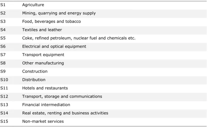
First, the data on production was determined per industry as well as the intermediate demand. At the European NUTS2 (regional) level, although there was no information available on output, we did obtain data on value added (VA) for 15 economic sectors, made available by Cambridge Econometrics (2008). Table 1 presents the classification for these 15 economic sectors.

Table 1. Industry classification in 15 sectors

S1 Agriculture

S2 Mining, quarrying and energy supply S3 Food, beverages and tobacco S4 Textiles and leather

S5 Coke, refined petroleum, nuclear fuel and chemicals etc. S6 Electrical and optical equipment

S7 Transport equipment

S8 Other manufacturing

S9 Construction

S10 Distribution

S11 Hotels and restaurants

S12 Transport, storage and communications S13 Financial intermediation

S14 Real estate, renting and business activities

S15 Non-market services

Maintaining the index g for products and introducing the index s for sectors, regional output and input were constructing using information on value added in the following way:

1 r r s N gs R gs k s k

VA

input

VA

=

∑

(16) 1 r r s N gs R gs k s k

VA

output

VA

=

∑

(17) This approach is based on two main assumptions. First, the technology through which a sector transforms inputs into outputs is assumed to be homogeneous throughout the country considered. The value added represents a good proxy for the magnitude of the industries inputs and outputs. It must be noted that this method maintains consistency per product, with the sum of output (or

(16)

16

input) per regional product equalling its national output, and per industry, with the regional shares of VA fixed at the original proportions.

Second, the preferences of final consumers in each region are assumed to reflect preferences nation-wide. The equation used for this part of the regionalisation is that presented in the introduction of this section and is as follows.

1 r r N g R g k k

HHD

=

∑

(14)3

Regional household demand was aggregated with the demand from non-profit organisations, because there was no regional information available on non-profit organisations. As their demand, on average, would be less than 2.5% of household demand, the latter makes up the main

component. Therefore, this aggregated category subsequently is referred to as household demand (HHD).

In order to regionalise the total government demand per region, we used data on value added non-market services (sector 15). This sector includes typical government activities, such as public administration, defence, education and health. It is reasonable to assume that this sector reflects how national government budgets are allocated. The demand pattern per product is assumed not to differ between regions, and is thus:

15 15 1 r r S N g R g k S k

VA

GOVD

VA

=

∑

(18) Gross capital formation is divided into three items: gross fixed capital formation, changes in inventories and changes in valuables. With respect to the first category, we proceeded as for government demand. Investments were considered per region, therefore:

1 r r N g R g k k

INV

=

∑

(19) Changes in inventories and valuables required more effort. In order to maintain full consistency between the regional and national accounts, the data in these two fluctuating and unpredictable columns had to be regionalised. The following observations were important in the regionalisation of these two accounts: 1) Changes in inventories are a more common phenomenon than changes in valuables. For valuables the changes are often small or even not included in the accounts of some countries; and 2) The changes in inventories and valuables were found to follow a similar pattern for the various goods and are combined in a subtotal under the name ‘changes in inventories and valuables’ in the ESA95 format. Given these observations, we decided to merge the two categories in a new aggregated column under the heading of inventories. Positive and negative changes in inventories would reflect supply excess or shortages, within the time period of one particular year. We assumed the demand for a certain product to have the same degree of fluctuation on a national level; therefore, producers per region were assumed to face excess or shortages of supply

proportional to their production levels. Hence, changes in inventories and valuables (CIV) were defined as: 1 r r N g R g k k

VA

CIV

VA

=

∑

(20)

(17)

17

In a similar fashion, this last consideration could also be applied to the two remaining columns in the Supply table: trade and transport margins (TTM) and taxes and subsidies (TAX). Since their regional variation is also assumed to be proportional to production, we defined them as:

1 r r N g R g k k

VA

TTM

VA

=

∑

and 1 r r N g R g k k

VA

TAX

VA

=

∑

(21)

2.2.2 Exports and Imports

In Section 2.2.1, all variables of the Supply and Use Tables are defined, with the exception of exports and imports. As mentioned before, we did not have any information available on regional exports and imports. However, we did have accurate information on regional production and consumption, per type of product, following the regionalisation. We used this information for a proportional allocation of exports to regional production and imports to regional demand. A simple example may illustrate the rationale behind this operation. Imagine that in a country N, industry s is agglomerated in one region (region r). From the national supply table it is known that this industry is providing a certain mix of products g as output. If country N is an exporter of these products, then exports must be brought in from the region where they are produced – in this case,region r. Naturally, full agglomeration of one industry almost never happens, but this reasoning, nonetheless, can be extended to less extreme cases. It therefore may safely be

assumed that the largest share of exports of a given product is produced in the region where most of these types of products are produced. A similar reasoning results in the following comparable conclusion with respect to imports. The largest share of imports of a given product is used in the region that uses the most of this product in intermediate or final use.

Hence, for every product g, we determined the regional production and consumption. These two figures, subsequently, were used to allocate national exports and imports to the different regions. Defining regional production and consumption is not as straightforward as it may seem. The general rule is that consumption (D) equals use minus exports (X), and production (Y) is supply minus imports (I). Hence:

r r r r r r r r

g g g gs g g g g

s

D Use

=

−

X

=

∑

Input

+

HHD GOVD INV

+

CIV

and (22)

r r r r r r

g g g gs g g

s

Y

=

Supply

−

I

=

∑

Output

+

TTM

+

TAX

However, there are some small, but important, corrections that must be taken into account. A change in inventories should be added to the production (in this period) although the demand does not take place until in the next period. Hence, negative entries under ‘changes in inventories and valuables’ are part of the supply and not a negative correction of the demand. In the same way, negative entries in trade and transport margins, as well as negative tax values (i.e. subsidies), are a positive demand instead of a negative supply. Once these corrections were applied, regional exports and imports were defined as follows:

1 r g r N g R g k g k

Y

X

Y

=

∑

and 1 r g r N g R g k g k

D

I

D

=

∑

(23) These regional exports and imports are a first estimate. Section 2.3 presents an adjustment using information on interregional and international transport flows. It must be emphasised that the exports and imports in Equation (0) refer to international trade. Products that are sold outside the producing region but within the same country are also exports from the region's perspective. We refer to this type of exports as intranational exports (IX) to avoid possible confusion. Similarly, we

(18)

18

use intranational imports (II) and, more generally, intranational trade. Section 2.2.3 is dedicated to intranational exports and intranational imports.

2.2.3 Cross-hauling and intranational trade

Information about the national share of products consumed and produced domestically was available, as data on re-exports were cleaned from the Supply and Use Tables (see Section 2.1.3). If the national production that is supplied to the national market is called own production (OY) and the national consumption of these products is own consumption (OD), we can write:

N N N N N N

g g g g g g

OY

=

Y

−

X

=

D

−

I

=

OD

(24) Own production and own consumption can be derived in two ways: either from production minus exports or from consumption minus imports. The two values, of course, are in fact the same.4

At the regional level, exports do not include intranational exports; therefore, the following slightly different relationship exists:

r r r r r

g g g g g

IY

=

OY

+

IX

=

Y

−

X

and

ID

_gr

=

OD II

_gr

+

_gr

=

D I

_gr

−

_gr

(25) with IY being production for domestic use and ID being demand for domestic products. Thus, IY is the production within a region, the resulting products of which either are sold within the same region (OY) or in other regions of the same country (intranational exports, IX). ID is the demand within a region, which is either being met by the production within the same region (OD) or by the production in other regions of the same country (intranational imports, II). Equation (0) shows that IY can be derived by subtracting exports (X) from production (Y), and ID by substracting imports (I) from consumption (D). Although production for domestic use and demand for domestic products are known, we did not know how many of the produced goods would remain in the producing region. Hence, we were unable to separate IY into its components own production (OY) and intranational exports (IX). Similarly, ID could also not be separated into own consumption (OD) and intranational imports (II).

Although, by definition, own production equals own consumption (OY=OD), it is likely that intranational exports, in actual practice, deviate from intranational imports. We therefore defined the domestic trade balance (IZ) as:

r r r g g g

IZ

=

ID

−

IY

(26)

which is also equal to the difference between intranational imports (II) and intranational exports (IX). A full regionalisation of Supply and Use Tables may be obtained assuming that there is no cross-hauling or trade between regions; this is described for the internal trade balance (IZ). However, cross-hauling is an important and sizeable empirical phenomenon that invalidates this type of regionalisation (see Kronenberg, 2009). Therefore, here, a theoretical model is presented that allows for cross-hauling. We subsequently used constraint nonlinear optimisation techniques to estimate the amount of cross-hauling in the 256 distinguished NUTS2 regions.

The Krugman (1991) model is the only theoretical international macromodel derived from

microeconomic behaviour that allows for cross-hauling. This approach is to be preferred5_because,

4 _{This happens automatically due to the way Use and Supply tables are constructed. In fact, as can}

be seen from Equations (0), Y = Supply - I and D = Use - X. In combination with Equation (0), then OY = Supply - I - X and OD = Use - X - I. Since Supply = Use, OY = OD. The corrections we applied in the previous section (on negative changes in inventories, negative trade and transport margins and subsidies) do not interfere with this line of reasoning.

(19)

19

if it is applied to all regions within a country, it (1) guarantees consistency with the national accounts and (2) is rigorously derived from microeconomic theory. For a more extensive explanation of the model, see Diodato and Thissen (WP, 2012). A concise description of the approach is given below.

The core of the model was built on the assumption that consumers love variety, and the demand for a variety of goods can be described by a Dixit-Stiglitz-Krugman demand function. This demand function is a CES function (constant elasticity of substitution) including (iceberg) transport costs to deal with the demand at different locations. This function describes that consumers are aware of small differences between products within the same product category, which they perceive as imperfect substitutes. Even though producers in every region use the same technology, the model differs from that of perfect competition, because consumers identify every variety as a unique product and, consequently, every producer has a certain degree of monopolistic power. The basic Dixit-Stiglitz monopolistic competition (Dixit and Stiglitz, 1977) has been extended by Krugman (1991) with iceberg-type transport costs (Samuelson, 1954) to build a spatial two-region model. We used this basic theoretical model to derive cross-hauling.

It is important to emphasise that we used a two-region model because we only wanted to

determine the amount of cross-hauling per region. We did not want to use the model to determine trade patterns. As explained before, using the model to estimate trade patters would make the data set useless for any further data analysis. The use of the Krugman model to determine only the amount of cross-hauling, therefore, was crucial in the presented approach.

In the two-region model, there was always one region under investigation (the focus region r) and the rest of the country h (the second region). This second region, therefore, differs for every focus region. Producers of product g were distributed over both regions. Consumers not only pay

interregional transport costs if products are imported from elsewhere in the country, but transport costs are also payable for products produced locally.6_{Given the theoretical model we therefore}

have intranational exports from region r to the rest of the country h equal to

1 1 1

(

)

(

)

(

)

r r rh h r h h r r hh rh

P T

IX

ID n

n P T

σ σ σ − − −

=

+

₍₂₇₎

And intranational imports into region r from the rest of the country h as:

1 1 1

(

)

(

)

(

)

h r hr r h r r h h rr hr

P T

II

ID n

n P T

σ σ σ − − −

=

+

₍₂₈₎

Where P represents price, n the number of firms, σ the elasticity of substitution and T the iceberg transport costs. The index g (product category) was omitted to simplify the equations.

With homogeneous technology this is:

r r r

IY

n

P

α

=

(29) With

α

equalling optimal output per variety, which in the model is the same for every producer, irrespective of location. Substitution of the number of varieties (0) in both Equations (0) and (0) led to a simplification of the intranational exports and imports. Combining Equations (0) and (0) resulted in two expressions that, after rearranging, resulted in expressions for intranational exports and intranational imports expressed as a function of value and not of price or quantity.

(20)

20

( , ,

,

)

r r h r h

IX

=

f T

σ

ID ID IZ

≡

II

and (30)

( , ,

,

)

r r h h h

II

=

f T

σ

ID ID IZ

≡

IX

Intranational imports (II) and exports (IX) are now functions of only two unknown quantities: transport costs and the elasticity of substitution7_{. Intranational trade can only be calculated if these}

two parameters are known. Since they were not, the problem had to be approached in a different way. The elasticity of substitution σ was taken from the literature, where it is commonly assumed to equal 1.5 (McKitrick, 1998). Transport costs were estimated (together with intranational trade) using non-linear programming.

Given the theoretical model described by Equation (0), we determined the optimal value for transportation costs

t

_rh between regions r and h in the non-linear optimisation, such that the national transport costs per product would be as close as possible to the national accounts’ data on trade and transport margins (TTM). In the optimisation we assumed a common transport cost function that is declining in transported distance according to a logarithmic relationship. The cross-hauling, or the total intranational trade per region, was endogenously determined in the procedure. Unfortunately, the data on trade and transport per product were limited to the national level, and the data were not always of a very high quality. We therefore expanded the methodology by including a second objective in the non-linear optimisation procedure based on cross-hauling, derived from freight data from the Dutch Ministry of Infrastructure and the Environment (2007). The data on cross-hauling derived from freight data is described by the share ChS of the total of the goods that are traded within regional borders divided by the goods sold to other regions. The data on services needed correction, since cross-hauling for this category is expected to be less important. The share for services is calculated as follows:

(

)

(

)

N N N g g g g services g services services goods r r _N _N _N g g g g goods g goods

Supply

X

Supply

ChS

Supply

X

Supply

∈ ∈ ∈ ∈

+

=

+

∑

(31)

The correction was based on a division that describes the relative propensity of exporting services in comparison to goods.

All described elements taken together lead to the following, non-linear minimisation problem that had to be solved to determine the amount of cross-hauling or, in other words, the share of products that were produced and used within the same region.

7_{The explicit functional forms is:}

2 2 2 2 2 2 2 2 2 2 2

[

]

(

)

4[

][

]

2(1

)

r rr hh h rh r rh r rh r rr hh h rh r rh r rh rr hh rh h r rh h r rh r h rh

IZ t t

ID t

IZ t

ID t

IZ t t

ID t

IZ t

ID t

t t

t

ID IZ t

ID ID t

IX

I

t

+

−

+

−

+

−

+

−

=

≡

−

(21)

21

(

)

(

)

[

]

(

)

1 1 2 2 1 2 2 2 2 2 2 2 2 2

. .

1 1 (

)

(

)

1 ln

(

)

(

)

(

) 0

r r r c rh rr c r c r c r r r r r rh rh rr hh rh r r rr hh h rh r rh r rh r h r rh h r rh

Min Objective Z Z

s t

Z

TTM

T

IX

T

IY

IX

Z

ChS IY

IY

IX

t

dist

t t

t IX

IZ t t

ID t

IZ t

ID t IX

ID IZ t

ID ID t

σ

β γ

− ∈ ∈

=

+





=

_

−

_









=

_

−

_

= +

+

−

+

−

+

−

=

∑

(32) In Equation (0) there are seven free variables, which needed to be determined: the objective variables (Z1 and Z2), the transportation variables (β, γ, t and T) and intranational exports (IX). All other elements are fixed parameters, whose values were taken from the available data sources. We used the conopt3 solver of the gams software to solve the problem described by Equation (0).

2.3 The origins and destinations of regional trade flows

This section describes how the origins and destinations of regional trade were determined. Data on goods and services were mainly derived from freight transport data and airline ticket information on first class and business class travel. The trade flows were determined by distributing the trade over the regions, given the amount produced and consumed in every region.

The determination of the amounts of goods and services produced and consumed per region is presented in the previous section. This provides the diagonal of the trade matrix. The number of products and services leaving and entering a region are also recorded in the regionalised Supply and Use Tables. These regional ‘exports’ were divided into international exports and intranational exports (destined for different regions within the same country).

In this section, the complete trade network between all distinguished NUTS2 regions is determined, given the intranational and international exports of the different regions. To determine export destinations, we used a simplified transport model, based on the probabilities of trade flows between different regions. These probabilities were derived from data on airline business trips (compare Derudder and Witlox, 2005), while for goods transport destinations the probabilities were based on freight transport data.

2.3.1 Transport hubs and the estimation of trade from transport data

The existence of transport hubs makes the derivation of trade data from transport data a complex procedure, as goods that are transported may be going to a transport hub instead of to their final destination. Therefore, there is a large difference between transport and trade data. We found that only 40% of all goods traded is being transported directly from origin to final destination. For the remaining 60%, at the least one transport hub is used before the final destination is reached. Especially in the case of international trade, it is likely that more than one hub is used: one in the country of origin and another in the country of destination.

The methodology used is based on a combination of two estimates on international trade between NUTS2 regions. The first estimate concerns the export of goods (the destination) and the second relates to their importation (the origin). We awarded both estimates a weight of 0.5 and minimised the quadratic difference between the final trade matrix and the two estimates. Below, the

methodology is first described for the destination (exports) of goods and services, followed by a description of the methodology to determine the trade based on the origin of imported goods. Both methods are similar, but for the latter destination probabilities are replaced by origin probabilities

Integrated Regional Europe