Natural Capital Model : Technical documentation of the quantification, mapping and monetary valuation of urban ecosystem services | RIVM

(1)

Natural Capital Model

Technical documentation of the

quantification, mapping and monetary

valuation of urban ecosystem services

RIVM Report 2017-0040

(2)

(3)

Natural Capital Model

Technical documentation of the quantification,

mapping and monetary valuation of urban ecosystem services

(4)

Colophon

Parts of this publication may be reproduced, provided acknowledgement is given to: National Institute for Public Health and the Environment, along with the title and year of publication.

DOI 10.21945/RIVM-2017-0040

R. Remme (auteur), RIVM T. de Nijs (auteur), RIVM M. Paulin (auteur), RIVM Contact:

Roy Remme DMG

roy.remme@rivm.nl

This investigation has been performed by order and for the account of the Ministry of LNV, within the framework of Doorontwikkeling TEEB-Stad

This is a publication of:

National Institute for Public Health and the Environment

P.O. Box 1 | 3720 BA Bilthoven The Netherlands

(5)

Synopsis

Natural Capital Model

Urban green and water (natural capital) is important for Dutch towns and cities. It contributes to a healthy, attractive living environment and has benefits for residents and companies. Urban green and water receive insufficient attention in city planning, compared to economic interests. The 'societal benefits' of urban green and water can be lost as a result. RIVM presents models that map eight social benefits of urban green and water.

The model captures the effects of green and water in terms of urban cooling, health, air quality, the effects of water and urban green on house prices, the effects of urban green on energy-saving due to the shelter provided by trees, energy generated from green waste

(pruning), wood production and lastly the presence of urban green in order to absorb carbon dioxide and counteract the effects of climate change. The models also show which effects urban development plans will have on the presence of greenery and water in towns and cities. The models are used for maps that have been developed for the Atlas of Natural Capital. They also provide input for the national Natural Capital Model. This national model is being developed so that the way the societal benefits are calculated is the same for each policy issue. RIVM has been asked to manage the calculation tool for the social benefits of urban green and water (TEEB-Stad) and is going to continue developing it. This report describes how the models have been

structured and which outcomes they generate. It describes the initial versions of the model and clarifies future developments of the Natural Capital Model.

Keywords: urban green and water, Natural Capital Model, natural capital, ecosystem services, spatial model, technical documentation

(6)

(7)

Publiekssamenvatting

Natural Capital Model

Groen en water (natuurlijk kapitaal) is belangrijk voor de Nederlandse steden. Het draagt bij aan een gezonde, aantrekkelijke leefomgeving en heeft voordelen voor bewoners en bedrijven. Bij stedelijk ontwikkeling is daar vaak onvoldoende aandacht voor en krijgen de economische

belangen voorrang. De ‘maatschappelijke baten’ van groen en water kunnen daardoor verloren gaan. Het RIVM presenteert modellen die acht maatschappelijke baten van stedelijk groen en water in beeld brengen. Het gaat om effecten van groen op de verkoeling van de stad, op de gezondheid, en op de luchtkwaliteit, effecten van water en groen op huizenprijzen, effecten van groen op energiebesparing door de beschutting van bomen, energieopwekking uit (snoei)restanten van groen, houtproductie, en ten slotte de aanwezigheid van groen om koolstofdioxide af te vangen om effecten van klimaatverandering tegen te gaan. De modellen geven ook aan welke effecten stedenbouwkundige plannen zullen hebben op de aanwezigheid van groen en water in

steden.

De modellen worden gebruikt voor de kaarten die zijn ontwikkeld voor de Atlas Natuurlijk Kapitaal. Ook leveren ze input voor het landelijke Natuurlijk Kapitaal Model. Dit landelijke model wordt ontwikkeld zodat de manieren om maatschappelijke baten te berekenen voor elke beleidsvraag hetzelfde zijn.

Het RIVM heeft de rekentool voor baten van groen en water in de stad (TEEB-Stad) in beheer gekregen en zal hem verder ontwikkelen. In dit rapport staat beschreven hoe de modellen zijn opgezet en welke uitkomsten de modellen leveren. De eerste versies van de modellen worden beschreven en toekomstige ontwikkelingen van het Natuurlijk Kapitaal Model worden belicht.

Kernwoorden: stedelijk groen, Natuurlijk Kapitaal Model, natuurlijk kapitaal, ecosysteemdiensten, ruimtelijk model, technische

(8)

(9)

Summary

Natural capital plays an essential role in our society by making

invaluable contributions to, for example, food production, reducing heat stress, carbon sequestration, drinking water production and nature recreation. These contributions are known as ecosystem services. Natural capital is under increasing pressure in urban areas, as cities continue to expand and become ever more compact. At the same time, natural capital provides multiple benefits to city dwellers, which is gaining increasing attention from urban planners and policy makers. Efforts to incorporate the improvement of natural capital and the development of urban green in urban planning are increasing. Location-based information on the benefits of natural capital in urban areas is often missing. To facilitate such efforts, spatially explicit urban natural capital models have been developed as a part of the Netherlands Natural Capital Model. The Natural Capital Model consists of baseline information on natural capital (input data) and separate sub-models for the different ecosystem services and societal benefits provided by natural capital. The sub-models together comprise the full model, which provides spatial information on a range of ecosystem services and connected benefits. The urban sub-models provide insight into the effects that changes in urban areas have on the benefits provided by urban natural capital. This report presents the technical descriptions of the first versions of eight urban sub-models of the Natural Capital Model, which have been developed as a part of the project ‘Doorontwikkeling TEEB-Stad’, by VITO (the Flemish institute for technological research) and the National Institute for Public Health and the Environment (RIVM). The project is an integral part of the City Deal ‘Waarde van groen en blauw in de stad’, in which a consortium of municipalities, knowledge partners, companies and NGOs work together to express the value of green and water in urban areas. This project aims to further develop the TEEB-Stad tool (www.teebstad.nl), a calculation tool to provide insight into the value of vegetation and water in urban planning projects. To enhance the TEEB-Stad tool, spatially explicit versions of the calculations have been developed to provide more accurate calculations for a specific location. These spatial calculations will form the basis for the spatially explicit version of the TEEB-Stad tool: the Green Benefit Planner. The Green Benefit Planner is a decision-support tool that calculates the effects of spatial planning on natural capital. The urban sub-models of the Natural Capital Model are applied in the first version of the Green Benefit

Planner. In addition, the urban models of the Natural Capital Model have been developed to improve ecosystem service maps for the Atlas of Natural Capital, a national atlas that provides maps on ecosystem services and natural capital in the Netherlands.

Five of the current sub-models are based on TEEB-Stad calculations and have been adapted in order to function with spatial data. These adapted sub-models are ‘air regulation’, ‘urban green and health effects’,

‘influence of urban green and water on residential property values’ and ‘energy savings in homes due to shelter provided by trees’. For these models, the reference values from the TEEB-Stad tool have been applied. The sub-models that were originally developed for the Atlas of

(12)

Natural Capital and that are presented here are ‘wood production’, ‘biomass for energy’, ‘carbon sequestration’ and ‘cooling by vegetation and water in urban areas’. To model the ecosystem services, publicly available maps and datasets have been used along with relevant scientific research. The Natural Capital Model provides maps as output that can be used to assess the current and potential future situations of urban natural capital.

The presented eight sub-models embody the core of Natural Capital Model for urban natural capital. Together, these sub-models provide planners with a broad overview of the benefits that natural capital can provide in urban areas. The Natural Capital Model is still in the

development phase and this report has described the initial set-up of eight sub-models. These models are ready to implement in spatial planning. Pilot projects are being carried out to apply and test the first version of the Natural Capital Model. These pilot projects will be used to further improve the sub-models and to expand the set of sub-models. The models will be further developed in collaboration with national partners (including the Netherlands Environmental Assessment Agency (PBL), Wageningen Environmental Research (WEnR) and Statistics Netherlands (CBS)) by integrating state-of-the-art national data and (inter)national scientific knowledge on the different ecosystem services. A collaborative Dutch Natural Capital Model has multiple advantages. The modelling results for different national institutes will have the same basis and therefore will not conflict. Also, collaboration will enhance the speed of model development and integrate a broader knowledge base. The approach will enhance overall support and the credibility of the model output. The set of urban ecosystem service models is expected to be extended in 2018. All presented models will be subject to

improvement based on newly available knowledge and data. The Natural Capital Model will gradually become a comprehensive national model that is applicable in a broad range of spatial planning issues and policy contexts.

(13)

1 Introduction

Natural capital plays an essential role in our society by making

invaluable contributions to, for example, food production, reducing heat stress, carbon sequestration, drinking water production and nature recreation. These contributions are known as ecosystem services (see Box 1 for further explanation of terminology). Natural capital is under increasing pressure in urban areas, as cities continue to expand and become ever more compact. At the same time, natural capital provides multiple benefits to city dwellers, which is gaining increasing attention from urban planners and policy makers. Urban green provides multiple benefits in cities, including public health benefits, recreation

opportunities, the reduction of pollutants, the reduction of heat stress and the provision of products, including food and raw materials. Efforts to incorporate the improvement of natural capital and the development of urban green in urban planning are increasing. Location-based

information on the benefits of natural capital in urban areas is often missing. To facilitate such efforts, urban natural capital models have been developed as a part of the Netherlands Natural Capital Model. These urban models provide insight into the effects that any changes in urban areas have on the benefits provided by urban natural capital. The Natural Capital Model is being developed to provide location-based spatial calculations of the benefits of natural capital for the Netherlands. The Natural Capital Model assesses the current provision of ecosystem services and the societal benefits from natural capital at the national level in order to inform policy makers, businesses and citizens. In addition, the model provides opportunities to calculate changes in

ecosystem service provision and the societal benefits in future scenarios. By feeding the model with altered input, such as spatial plans, future scenarios can be calculated. Such information is highly relevant for decision makers involved spatial planning, such as local and regional governments, city planners and landscape architects. Currently,

information on natural capital and ecosystem services is rarely included in spatial planning in the Netherlands. The development of the Natural Capital Model provides tools with which to explore these possibilities and ensure that decision makers can make more balanced assessments when assessing the sustainability and economic implications of a plan. In this report, we present the models for urban areas that have been developed as a part of the project ‘Doorontwikkeling TEEB-Stad’. The project is an integral part of the City Deal ‘Waarde van groen en blauw in de stad’, in which a consortium of municipalities, knowledge partners, companies and NGOs work together to express the value of green and water in urban areas. This project aims to further develop the TEEB-Stad tool (www.teebstad.nl), a calculation tool to provide insight into the value of vegetation and water in urban planning projects. To enhance the TEEB-Stad tool, spatially explicit versions of the calculations have been developed to provide more accurate calculations for a specific location. These spatial calculations will form the basis for the spatially explicit version of the TEEB-Stad tool: the Green Benefit Planner. The Green Benefit Planner is a decision-support tool that calculates the

(14)

effects of spatial planning on natural capital. The urban sub-models of the Natural Capital Model are applied in the first version of the Green Benefit Planner. In addition, the urban models of the Natural Capital Model have been developed to improve ecosystem service maps for the Atlas of Natural Capital, a national atlas that provides maps on

ecosystem services and natural capital in the Netherlands. The Atlas of Natural Capital provides maps of the Dutch natural capital based on current scientific knowledge. The Natural Capital Model will be used to systematically map and update the current state of Dutch natural capital and will model the flows that result from this natural capital.

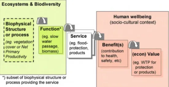
The Natural Capital Model consists of baseline information on natural capital (input data) and separate sub-models for the different ecosystem services and the societal benefits provided by natural capital. Taken together, the sub-models comprise the full model, which provides spatial information on a range of ecosystem services and connected benefits. These models produce maps that are in line with the cascade model for ecosystem services (Figure 1.1, developed by Haines-Young & Potschin, 2010). Biophysical processes, in combination with socio-economic input, are used to model the ecosystem services, which leads to societal benefits. These benefits are then modelled as monetary values of the services. The full model will be capable of spatially modelling both urban and rural ecosystem services, depending on the wishes of the user. The presented ecosystem service models have been developed by VITO (the Flemish institute for technological research) together with the National Institute for Public Health and Environment (RIVM). In this report, the technical documentation of the models for the urban ecosystem services will be presented. Urban ecosystem services focus predominantly on providing a clean and healthy living environment for inhabitants (e.g. reducing heat stress, improving property values and improving the energy efficiency of cities). In addition, urban areas also provide services that are provided by more rural areas as well, such as carbon sequestration and the production of biomass for energy production (for example from urban forests).

(15)

This report describes the first versions of the first eight sub-models and provides a baseline for the urban ecosystem services in the Natural Capital Model. As the Natural Capital Model develops, the sub-models will be improved as new data and knowledge becomes available and additional sub-models may be added. Five of the current sub-models are based on TEEB-Stad calculations and have been adapted in order to function with spatial data. These adapted sub-models are ‘air

regulation’, ‘urban green and health effects’, ‘influence of urban green and water on residential property values’ and ‘energy savings in homes due to shelter provided by trees’. For these models, the reference values from the TEEB-Stad tool have been applied. Sub-models that were originally developed for the Atlas of Natural Capital and are presented here are ‘wood production’, ‘biomass for energy’, ‘carbon sequestration’ and ‘cooling by vegetation and water in urban areas’. To model the ecosystem services, publicly available maps and datasets have been used along with relevant scientific research. The Natural Capital Model provides maps as output. All sub-models were calculated on a 10x10m grid size for the whole of the Netherlands. All monetary values have been corrected to 2016 € values, based on the Consumer Price Index (CPI)1. This report presents the technical documentation of each model, but does not present model output or simulations that are done with the model. Output maps and further information on the Natural Capital Model can be found on the Atlas of Natural Capital website:

www.atlasnaturalcapital.nl.

Each sub-model provides at least one, but usually multiple output maps, presenting monetary value, relevant actual biophysical flows and, in several cases, potential provision. The maps are produced in various stages in each sub-model. Output maps can be both end-points and mid-points. In the latter case, the output maps are used in further calculations of the sub-model. Each chapter of this report presents a sub-model, describing the steps that have been taken to develop the model, the input data used, the output maps the models produce and the scientific knowledge that has been incorporated. The models are presented in a bottom-up manner, presenting the final map and moving back through the model to describe each step that was necessary to produce this map, and describing the production of the maps preceding the final map. Most model descriptions can be read as stand-alone technical descriptions, with the exception of the ‘biomass for energy’ model (Chapter 3) and the ‘carbon sequestration’ model (Chapter 4), which use maps from the ‘wood production’ model (Chapter 2) as input.

1_{Derived from CBS, 2018. StatLine, annual rate of change CPI; since 1963. Retrieved}

from:

http://statline.cbs.nl/Statweb/publication/?DM=SLEN&PA=70936eng&D1=0&D2=493,506, 519,532,545,558,571,584,597,610,623,636,649,662,675,688,701,l&LA=EN&HDR=T&STB =G1&VW=T

(16)

Box 1: Glossary with key terms

This box presents an overview of the key terms that are applied in this report. Terminology is applied as defined by the H2020 ESMERALDA project on mapping and assessing European ecosystem services (Potschin & Burkhard, 2015), unless stated otherwise.

Term Definition

Actual ecosystem

service The rate at which ecosystem services are supplied to some beneficiary (cf. ‘ecosystem service flow’ in Potschin & Burkhard, 2015). Biophysical

suitability A relative score to assess the capacity of an area to provide an ecosystem service based on biophysical environmental variables, such as soil information, groundwater level and climate.

Benefits Positive change in well-being from the fulfilment of needs and wants (TEEB, 2010). Ecosystem service The direct and indirect contributions of

ecosystems to human well-being (TEEB, 2010).

Green infrastructure A strategically planned network of natural and semi-natural areas with other environmental features designed and managed to deliver a wide range of ecosystem services (ES). It incorporates green spaces (or blue spaces if aquatic ecosystems are concerned) and other physical features in terrestrial (including coastal) and marine areas. On land, green infrastructure is present in rural and urban settings.

Monetary valuation The process whereby people express the importance or preference they have for the service or benefits that ecosystems provide in monetary terms.

Natural capital The elements of nature that directly or indirectly produce value for people, including ecosystems, species, fresh water, land, minerals, air and oceans, as well as natural processes and functions. The term is often used synonymously with natural asset, but in general implies a specific component.

Potential ecosystem

service The hypothetical maximum yield of selected ecosystem services (cf. ‘ecosystem service potential’ in Potschin & Burkhard, 2015). Urban green All vegetated areas (both public and private) in

and directly surrounding areas with medium to high population densities. Urban green

includes large vegetated areas such as parks and urban forests, as well as flower beds, street trees and private gardens.

(17)

2 Wood production

2.1 Overview

Forest biomass provides a range of ecosystem services, e.g. through the provision of round wood for construction and furniture production. The ‘wood production’ ecosystem service model calculates round wood production that is used to produce wood products. Although there are fewer productive forests in urban areas than in rural areas, some city trees can also be used in the context of wood production. In addition, the wood production model is a necessary input for two other models: biomass production for energy and carbon sequestration. For this reason, the model has been included in the urban ecosystem service set.

Four output maps (i.e. actual wood production, biophysical suitability for wood production, the monetary value of actual wood production,

potential wood production) have been produced for the ecosystem service ‘wood production’ (see Table 2.1). These maps have been produced to show what the capacity of an area is for wood production (suitability and potential), given environmental characteristics and how much is actually growing in an area (actual production and the

incremental monetary value). The biophysical suitability and potential wood production maps are included in the model output to provide insight into which areas can potentially provide higher service flows, which can facilitate spatial planning processes.

The output map has been produced by combining existing spatial data for the Netherlands with maps developed by RIVM for the Natural Capital Model. Tables 2.1 and 2.2 provide an overview of the input and output maps to model the ecosystem service ‘wood production’. The original input maps for groundwater levels and soil biophysical units (Alterra, 2006 and Alterra, 2016) contained data gaps for most built-up areas. These maps have been adjusted to cover urban areas as well, using additional datasets from TNO (2015).

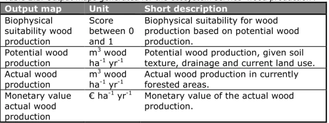
Table 2.1. Output maps generated for the ecosystem service ‘wood production’.

Output map Unit Short description

Biophysical suitability wood production Score between 0 and 1

Biophysical suitability for wood production based on potential wood production.

Potential wood production m

3_wood

ha-1_yr-1 Potential wood production, given soil _{texture, drainage and current land use.} Actual wood

production m

3_wood

ha-1_yr-1 Actual wood production in currently _{forested areas.} Monetary value

actual wood production

€ ha-1_yr-1_{Monetary value of the actual wood} production.

(18)

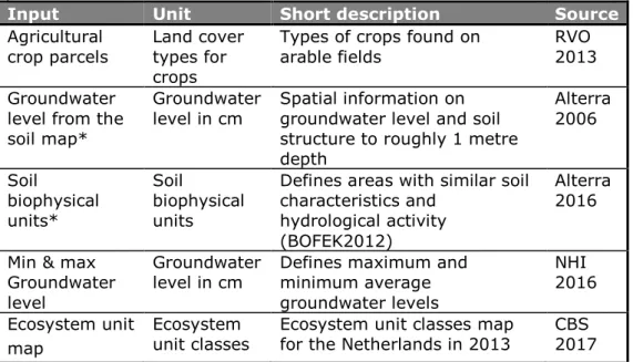
Table 2.2. Input maps applied to estimate the ecosystem service ‘wood production’.

Input Unit Short description Source

Agricultural

crop parcels Land cover types for crops

Types of crops found on

arable fields RVO 2013 Groundwater

level from the soil map*

Groundwater

level in cm Spatial information on groundwater level and soil structure to roughly 1 metre depth Alterra 2006 Soil biophysical units* Soil biophysical units

Defines areas with similar soil characteristics and

hydrological activity (BOFEK2012)

Alterra 2016 Min & max

Groundwater level

Groundwater

level in cm Defines maximum and minimum average groundwater levels NHI 2016 Ecosystem unit map Ecosystem

unit classes Ecosystem unit classes map for the Netherlands in 2013 CBS 2017

*The original maps have been supplemented with data from TNO (2015), so that the maps also fully cover urban areas.

2.2 Modelling the ecosystem service

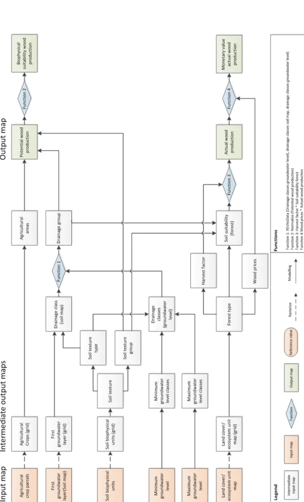
The service ‘wood production’ results in four output maps. The modelling of these four maps is described in the following sections. Figure 2.2 provides a schematic overview of the way input data has been modelled in order to produce the output maps for the ecosystem service ‘wood production.’

2.2.1 Monetary value of actual wood production

The monetary value of the actual wood production is calculated according to (Function 4, Figure 2.2):

𝑴𝑴𝑴𝑴𝑴𝑴𝑴𝑴𝑴𝑴𝑴𝑴𝑴𝑴𝑴𝑴 𝒗𝒗𝑴𝑴𝒗𝒗𝒗𝒗𝑴𝑴 𝑴𝑴𝒐𝒐 𝒘𝒘𝑴𝑴𝑴𝑴𝒘𝒘 𝒑𝒑𝑴𝑴𝑴𝑴𝒘𝒘𝒗𝒗𝒑𝒑𝑴𝑴𝒑𝒑𝑴𝑴𝑴𝑴 = 𝒘𝒘𝑴𝑴𝑴𝑴𝒘𝒘 𝒑𝒑𝑴𝑴𝒑𝒑𝒑𝒑𝑴𝑴 × 𝑴𝑴𝒑𝒑𝑴𝑴𝒗𝒗𝑴𝑴𝒗𝒗 𝒘𝒘𝑴𝑴𝑴𝑴𝒘𝒘 𝒑𝒑𝑴𝑴𝑴𝑴𝒘𝒘𝒗𝒗𝒑𝒑𝑴𝑴𝒑𝒑𝑴𝑴𝑴𝑴 Given the available information on forest cover in the Netherlands, a distinction is made between three forest types: coniferous, deciduous and mixed forest. The average wood price, based on data provided by Demey et al. (2013) and Liekens et al. (2013), has been estimated as 46.15 €/m3_{for coniferous, 42.63 €/m}3_{for deciduous and 44.39 €/m}3 _for mixed wood (corrected from 2010 to 2016 € value).

2.2.2 Actual wood production

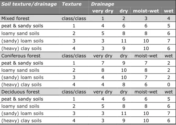
The actual wood production depends on the annual increment and the fraction of wood that is harvested per year (Function 3, Figure 2.2): 𝑨𝑨𝒑𝒑𝑴𝑴𝒗𝒗𝑴𝑴𝒗𝒗 𝒘𝒘𝑴𝑴𝑴𝑴𝒘𝒘 𝒑𝒑𝑴𝑴𝑴𝑴𝒘𝒘𝒗𝒗𝒑𝒑𝑴𝑴𝒑𝒑𝑴𝑴𝑴𝑴 = 𝑴𝑴𝑴𝑴𝑴𝑴𝒗𝒗𝑴𝑴𝒗𝒗 𝒑𝒑𝑴𝑴𝒑𝒑𝑴𝑴𝑴𝑴𝒊𝒊𝑴𝑴𝑴𝑴𝑴𝑴 × 𝒉𝒉𝑴𝑴𝑴𝑴𝒗𝒗𝑴𝑴𝒉𝒉𝑴𝑴 𝒐𝒐𝑴𝑴𝒑𝒑𝑴𝑴𝑴𝑴𝑴𝑴 The fraction harvested (harvest factor) is based on the 6th_National Forest Inventory and is estimated as: 0.373 for deciduous, 0.531 for coniferous and 0.466 for mixed forest (Schelhaas et al., 2014). The annual increment can be estimated, given specific soil texture and soil

(19)

drainage groups, for different forest types (Table 2.3) according to Vandekerkhove et al. (2014).

Soil texture

Four soil texture groups have been defined, based on the texture codes given in the map with the soil biophysical units (BOFEK2012, see Alterra 2016). These four texture groups have been grouped into two texture types: light soils and heavy soils, used for the definition of the drainage classes. Table 2.4 gives the reclassification of the soil types found in the map with the soil biophysical units (BOFEK2012) into eight main texture classes. Table 2.5 shows the reclassification of these 8 texture classes into 4 texture groups and two texture types.

Soil drainage

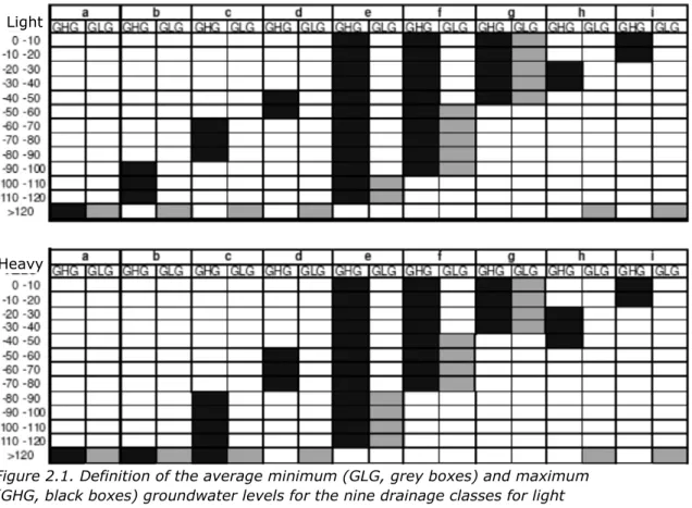
Input maps with the average minimum (GLG) and maximum (GHG) groundwater level (NHI, 2006) have been reclassified into nine soil drainage classes, according to Finke et al. (2010) as given in Figure 2.1. As the groundwater level maps do not cover the Wadden islands in the north of the Netherlands, the groundwater level from the soil map has been reclassified into the same nine hydrological classes according to a reclassification table based on expert judgement (available on request). In both cases, a distinction has been made between two texture types: light soils and heavy soils as defined in Table 2.5. The nine drainage classes have been regrouped into four drainage groups according to Table 2.6 in order to estimate the annual increment.

Table 2.3. Wood increment (m3_{/ha/yr) per soil texture and drainage class}

combination for three forest types.

Soil texture/drainage Texture Drainage

very dry dry moist-wet wet

Mixed forest class/class 1 2 3 4

peat & sandy soils 1 4 6 6 5

loamy sand soils 2 5 8 8 6

(sandy) loam soils 3 3 11 10 7

(heavy) clay soils 4 3 9 10 6 Coniferous forest class/class very dry dry moist-wet wet

(heavy) clay soils 4 4 8 6 0 Deciduous forest class/class very dry dry moist-wet wet

(20)

Table 2.4. Reclassification of the soil classes from the BOFEK map (soil physical properties) into soil texture classes.

BOFEK

Code Texture BOFEK Code Texture BOFEK Code Texture BOFEK Code Texture

101 V 303 S 321 S 412 E 102 V 304 Z 322 Z 413 E 103 V 305 Z 323 Z 414 E 104 V 306 Z 324 Z 415 U 105 V 307 S 325 S 416 L 106 V 308 S 326 Z 417 L 107 V 309 Z 327 Z 418 E 108 V 310 Z 401 E 419 E 109 V 311 Z 402 E 420 E 110 V 312 S 403 E 421 E 201 U 313 S 404 U 422 U 202 E 314 S 405 U 501 E 203 V 315 S 406 L 502 L 204 V 316 S 407 E 503 U 205 Z 317 S 408 L 504 L 206 Z 318 S 409 L 505 L 301 Z 319 S 410 E 506 L 302 Z 320 Z 411 E 507 A

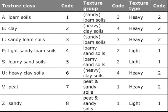
Table 2.5. Classification of soil texture classes into four texture groups and two texture types.

Texture class Code Texture _group Code Texture _type Code

A: loam soils 1 (sandy) _{loam soils} 3 Heavy 2

E: clay 2 (heavy) _{clay soils} 4 Heavy 2

L: sandy loam soils 3 (sandy) _{loam soils} 3 Heavy 2

P: light sandy loam soils 4 loamy _{sand soils} 2 Light 1

S: loamy sand soils 5 loamy _{sand soils} 2 Light 1

U: heavy clay soils 6 (heavy) _{clay soils} 4 Heavy 2

V: peat 7 peat & sandy

soils 1 Heavy 2

Z: sandy 8 peat & sandy

(21)

Figure 2.1. Definition of the average minimum (GLG, grey boxes) and maximum (GHG, black boxes) groundwater levels for the nine drainage classes for light (sandy & loamy soils) and heavy (clay & peaty) soils according to Finke et. al. (2010).

Table 2.6 Information from ‘Drainage group’ knowledge table necessary for reclassification (Function 1, Figure 2.2).

Drainage class Description Drainage group Code

A excessively drained soils _{(very dry)} Very dry 1 B well-drained soils (dry) Dry 2 C moderately well-drained _{soils (medium dry)} Dry 2 D insufficiently drained soils _{(moderately wet)} Moist-wet 3 E rather poorly drained soils with groundwater

permanently (wet) Moist-wet 3

F poorly drained soils with groundwater permanently

(very wet) Wet 4

G extremely poorly drained _{soils (very wet)} Wet 4 H poorly drained soils with backwater (temporary

groundwater) (very wet) Moist-wet 3

I rather poorly drained soils with backwater (temporary

groundwater) (wet) Wet 4

Light

(22)

Table 2.7. Applied maximum growth rates (m3_{/ ha. year) for the agricultural and}

non-agricultural soils for various drainage and texture classes according to Vandekerkhove et al., (2014).

Non-agricultural soils

Texture / Drainage Very dry dry moist-wet wet

peat & sandy soils 12 16 9 6

loamy sand soils 12 16 12 11

(sandy) loam soils 10 16 18 9

(heavy) clay soils 10 15 20 7

Agricultural soils

Texture / Drainage Very dry dry moist-wet wet

peat & sandy soils 15 20 12 9

loamy sand soils 15 20 15 14

(sandy) loam soils 11 18 20 12

(heavy) clay soils 11 17 22 9

2.2.3 Potential wood production

The simulation of the potential wood production [m3_{/ha. year] is based} on Vandekerkhove et al. (2014). According to this study, the potential wood production differs between agricultural soils that have been fertilized and non-agricultural soils as shown in Table 2.7. For each texture group and drainage group, the most productive tree species has been selected to calculate potential wood production. The locations of the agricultural areas are based on the input map with the agricultural crop parcels. Given the crop-type, the parcels are reclassified as agricultural; the rest of the area is defined as non-agricultural.

2.2.4 Biophysical suitability for wood production

The map with the potential wood production is normalized to generate the map with the biophysical suitability for wood production as follows (Function 2, Figure 2.2):

𝑩𝑩𝒑𝒑𝑴𝑴𝒑𝒑𝒉𝒉𝑴𝑴𝒉𝒉𝒑𝒑𝒑𝒑𝑴𝑴𝒗𝒗 𝒉𝒉𝒗𝒗𝒑𝒑𝑴𝑴𝑴𝑴𝒔𝒔𝒑𝒑𝒗𝒗𝒑𝒑𝑴𝑴𝑴𝑴 𝒐𝒐𝑴𝑴𝑴𝑴 𝒘𝒘𝑴𝑴𝑴𝑴𝒘𝒘 𝒑𝒑𝑴𝑴𝑴𝑴𝒘𝒘𝒗𝒗𝒑𝒑𝑴𝑴𝒑𝒑𝑴𝑴𝑴𝑴 = 𝒑𝒑𝑴𝑴𝑴𝑴𝑴𝑴𝑴𝑴𝑴𝑴𝒑𝒑𝑴𝑴𝒗𝒗 𝒘𝒘𝑴𝑴𝑴𝑴𝒘𝒘 𝒑𝒑𝑴𝑴𝑴𝑴𝒘𝒘𝒗𝒗𝒑𝒑𝑴𝑴𝒑𝒑𝑴𝑴𝑴𝑴

/ 𝒊𝒊𝑴𝑴𝒎𝒎𝒑𝒑𝒊𝒊𝒗𝒗𝒊𝒊 𝑴𝑴𝒐𝒐 𝑴𝑴𝒉𝒉𝑴𝑴 𝒊𝒊𝑴𝑴𝒑𝒑 𝒘𝒘𝒑𝒑𝑴𝑴𝒉𝒉 𝑴𝑴𝒉𝒉𝑴𝑴 𝒑𝒑𝑴𝑴𝑴𝑴𝑴𝑴𝑴𝑴𝑴𝑴𝒑𝒑𝑴𝑴𝒗𝒗 𝒘𝒘𝑴𝑴𝑴𝑴𝒘𝒘 𝒑𝒑𝑴𝑴𝑴𝑴𝒘𝒘𝒗𝒗𝒑𝒑𝑴𝑴𝒑𝒑𝑴𝑴𝑴𝑴

2.3 Remarks and points for improvement

• The new data on vegetation (Appendix I, coverage of each grid cell with trees and tree height) could be combined with

information on forest type from the LCEU map and incorporated into the model.

• The National Forest Inventory (Nederlandse Bosinventarisatie, NBI) could be used to improve the input maps. The 6th_National Forest Inventory (Schelhaas et al., 2014) was finished in 2014, providing statistical data for approximately 3,000 sites. More comprehensive was the 4th_{NBI (then named Bosstatistiek), but} the dataset is older (1980s). The 6th_{NBI can be found by clicking} on the following link:

http://www.probos.nl/publicaties/overige/1094-mfv-2006-nbi-2012. CBS and Wageningen University & Research have

(23)

developed a wood production model based on the 6th_{NBI data} that should be compared (and possibly integrated) with this model.

• The national model STONE (Wolf et al. 2003) can be used to incorporate fertilization data (N and P). This is preferable to the current reclassification made using the LCEU dataset.

• Currently, Belgian data on wood prices is used. Wageningen Economic Research also provides similar data that could be used in future versions of the model. See:

http://agrimatie.nl/Binternet_Bosbouw.aspx?ID=1005&Lang=0& sectorID=3303

2.4 References

• Alterra 2006. Bodemkaart van Nederland 1:50000. Available at

http://www.nationaalgeoregister.nl/geonetwork/srv/dut/catalog.s

earch#/metadata/1032583a-1d76-4cf8-a301-3670078185ac?tab=contact

• Alterra 2016. Bodemfysische Eenhedenkaart (BOFEK 2012). Available at https://www.wur.nl/nl/show/Bodemfysische-Eenhedenkaart-BOFEK2012.htm

• CBS 2017. Ecosystem Unit map, 2013. Available at

https://www.cbs.nl/en-gb/background/2017/12/ecosystem-unit-map

• Demey, A., Baeten, L., and Verheyen, K., 2013. Opbouw methodiek prijsbepaling hout. ANB. Brussels, Belgium.

• Finke, P.A., Van de Wauw, J. and Baert, G., 2010. Ontwikkelen en uittesten van een methodiek voor het actualiseren van de drainageklasse van de bodemkaart van Vlaanderen. Universiteit Gent, vakgroep Geologie en Bodemkunde.

• Liekens, I., Van der Biest, K., Staes, J., De Nocker, L., Aertsens, J., & Broekx, S., 2013. Waardering van ecosysteemdiensten, een handleiding. VITO. Mol.

• NHI, 2006. GxG kaarten, Gemiddelde Grondwaterstanden van modelversie LHM 3.0.2 voor 1998-2006. Available at

http://www.nhi.nu/nl/index.php/data/

• RVO 2013. Basisregistratie Gewaspercelen (BRP), 2013. Available at

earch#/metadata/%7B25943e6e-bb27-4b7a-b240-150ffeaa582e%7D

• Schelhaas, M.J., Clerkx, A.P.P.M., Daamen, W.P., Oldenburger, J.F., Velema, G., Schnitger, P., Schoonderwoerd, H. & Kramer, H., 2014. Zesde Nederlandse Bosinventarisatie. Methoden en basisresultaten. Wageningen, Alterra Wageningen UR, Alterra-rapport 2545.

• TNO, 2015. Oppervlaktegeologie, geologische kaart onder INSPIRE. Available at

earch#/metadata/80630ee7-3a15-4ea0-bdc0-a8aebfa2f204?tab=relations

• Van de Walle I., van Camp N., Perrin D., Lemeur R., Verheyen K., van Wesemael B., Laitat E., 2005. Growing stock-based assessment of the carbon stock in the Belgian forest biomass. Annals of Forest Science 62: 1-12.

(24)

• Vandekerkhove, K., De Keersmaeker, L., Demolder, H., Esprit, M., Thomaes, A., Van Daele, T., & Van der Aa, B., 2014.

Hoofdstuk 13 - Ecosysteemdienst houtproductie. In M. Stevens (Ed.), Natuurrapport - Toestand en trend van ecosystemen en ecosysteemdiensten in Vlaanderen. Brussels: Instituut voor Natuur-en Bosonderzoek.

• Wolf, J., Beusen, A.H.W., Groenendijk, P., Kroon, T., Rötter, R., van Zeijts, H., 2003. The integrated modeling system STONE for calculating nutrient emissions from agriculture in the

(25)

(26)

(27)

3 Biomass for energy

Biomass is the general name given to organic material from plants and animals. Nature produces biomass in the form of wood and plants, for example. The agricultural industry also produces biomass in forms such as animal feed, crop residues, straw and manure. Biomass may be in an unprocessed form (e.g. tree trunks) or a processed form (furniture or paper). Biomass can be used for a variety of purposes, including agricultural fertilization, manufacturing and energy generation. This model focusses on the use of biomass for energy production purposes. The energy extracted from biomass is known as bio-energy and it may be used as electricity, heat or gas. Biomass-based energy is obtained by the combustion, gasification or fermentation of the biomass. Biomass that people eat is not referred to within the ecosystem service

classification system as biomass, but rather as food, and is not included in this sub-model.

At the current stage, five output maps (i.e. actual production from crops, actual production from forests, potential energy production from crops, potential energy production from cultivated grassland, potential energy production from forests) have been produced for the Atlas of Natural Capital for the ecosystem service ‘biomass for energy’. Tables 3.1 and 3.2 provide an overview of the input and output maps to model the ecosystem service ‘biomass for energy production’. These maps have been produced to show what the capacity of an area is for energy production from biomass (potential maps) given the environmental characteristics and how much is actually being produced in an area (actual production). The potential biomass production maps are included in the model output to provide insight into which areas can potentially provide higher service flows, which can facilitate spatial planning processes.

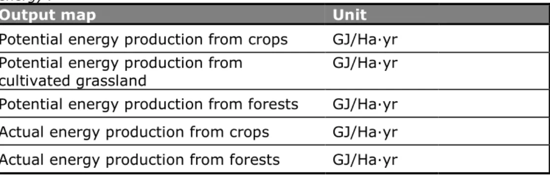
Table 3.1. Output maps generated for the ecosystem service ‘biomass for energy’.

Output map Unit

Potential energy production from crops GJ/Ha·yr Potential energy production from

cultivated grassland GJ/Ha·yr

Potential energy production from forests GJ/Ha·yr Actual energy production from crops GJ/Ha·yr Actual energy production from forests GJ/Ha·yr

(28)

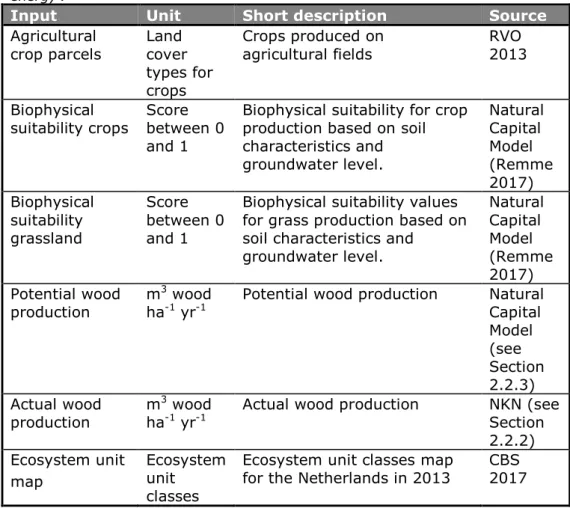
Table 3.2. Input maps applied to estimate the ecosystem service ‘biomass for energy’.

Agricultural

crop parcels Land cover types for crops

Crops produced on

agricultural fields RVO 2013 Biophysical

suitability crops Score between 0 and 1

Biophysical suitability for crop production based on soil characteristics and groundwater level. Natural Capital Model (Remme 2017) Biophysical suitability grassland Score between 0 and 1

Biophysical suitability values for grass production based on soil characteristics and

groundwater level. Natural Capital Model (Remme 2017) Potential wood production m 3_wood

ha-1_yr-1 Potential wood production Natural _Capital Model (see Section 2.2.3) Actual wood production m 3_wood

ha-1_yr-1 Actual wood production NKN (see _Section 2.2.2) Ecosystem unit map Ecosystem unit classes

Ecosystem unit classes map

for the Netherlands in 2013 CBS 2017

The service biomass for energy production results in five output maps. The modelling of these maps is based on the NARA study conducted by Van Kerckvoorde & Van Reeth (2014) and is the described in the

following sections. Figure 3.1 provides a schematic overview of the way input data has been modelled in order to produce the output maps for this ecosystem service.

3.2.1 Potential energy production from crops and cultivated grassland

The potential energy production from crops and permanent cultivated grassland is estimated according to (Function 1 and Function 2, Figure 3.1):

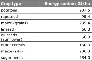
𝑷𝑷𝑴𝑴𝑴𝑴𝑴𝑴𝑴𝑴𝑴𝑴𝒑𝒑𝑴𝑴𝒗𝒗 𝑴𝑴𝑴𝑴𝑴𝑴𝑴𝑴𝒆𝒆𝑴𝑴 𝒑𝒑𝑴𝑴𝑴𝑴𝒘𝒘𝒗𝒗𝒑𝒑𝑴𝑴𝒑𝒑𝑴𝑴𝑴𝑴 = 𝑩𝑩𝒑𝒑𝑴𝑴𝒑𝒑𝒉𝒉𝑴𝑴𝒉𝒉𝒑𝒑𝒑𝒑𝑴𝑴𝒗𝒗 𝒉𝒉𝒗𝒗𝒑𝒑𝑴𝑴𝑴𝑴𝒔𝒔𝒑𝒑𝒗𝒗𝒑𝒑𝑴𝑴𝑴𝑴 × 𝑴𝑴𝑴𝑴𝑴𝑴𝑴𝑴𝒆𝒆𝑴𝑴 𝒑𝒑𝑴𝑴𝑴𝑴𝑴𝑴𝑴𝑴𝑴𝑴𝑴𝑴 The biophysical suitability maps for crops and permanent grassland form an output from the ecosystem service ‘food production’ (see Remme, 2017 for technical description). The biophysical suitability maps show the suitability of areas for crop production based on soil characteristics and groundwater level, regardless of the current land use. The energy content for permanent grassland is 111.2 GJ/ha according to the Phyllis database (www.ecn.nl/phyllis). For crops, the energy content is

(29)

assumed to be 157.8 GJ/ha based on the average energy content of crops as shown is Table 3.3 (Van Kerckvoorde & Van Reeth 2014). Table 3.3. Energy content of crops based on Van Kerckvoorde & Van Reeth (2014).

Crop type Energy content GJ/ha

potatoes 207.5 rapeseed 95.4 maize (grains) 235.4 linseed 66.3 oil seeds (sunflower) 66.3 other cereals 130.9 maize (silo) 206.3 sugar beets 254.0

3.2.2 Actual energy production from crops and cultivated grassland

The actual energy production from crops and cultivated grassland is based on the maps for the potential energy production from crops and grassland and the parcels where these crops are currently being grown for energy production. The map filters out all other parcels that are currently not being used for energy crops. Given the map with agricultural crop parcels, the following crops have been selected as energy crops: miscanthus (elephant grass), linseed, rapeseed, maize for energy and fast-growing trees with short turnover time (e.g. willow coppice). Some crops, such as potatoes and sugar beets, have residual flows that are used for energy production. These are not included in this estimate.

3.2.3 Potential energy production from forests

The potential energy production from forests estimates the total annual energy increment of the aboveground biomass, except for the stem wood (stem wood and branches with a diameter > 7 cm). This estimate is based on the potential wood production in which the annual increase in stem wood is estimated for the optimal tree type given the local soil and drainage class. To estimate the potential energy production from forests, the following equation is used (Function 3, Figure 3.1):

𝑷𝑷𝑴𝑴𝑴𝑴𝑴𝑴𝑴𝑴𝑴𝑴𝒑𝒑𝑴𝑴𝒗𝒗 𝑴𝑴𝑴𝑴𝑴𝑴𝑴𝑴𝒆𝒆𝑴𝑴 𝒑𝒑𝑴𝑴𝑴𝑴𝒘𝒘𝒗𝒗𝒑𝒑𝑴𝑴𝒑𝒑𝑴𝑴𝑴𝑴

= 𝑷𝑷𝑴𝑴𝑴𝑴𝑴𝑴𝑴𝑴𝑴𝑴𝒑𝒑𝑴𝑴𝒗𝒗 𝒘𝒘𝑴𝑴𝑴𝑴𝒘𝒘 𝒑𝒑𝑴𝑴𝑴𝑴𝒘𝒘𝒗𝒗𝒑𝒑𝑴𝑴𝒑𝒑𝑴𝑴𝑴𝑴 × 𝑾𝑾𝑴𝑴𝑴𝑴𝒘𝒘 𝑴𝑴𝑴𝑴𝑴𝑴𝑴𝑴𝒆𝒆𝑴𝑴 𝒑𝒑𝑴𝑴𝑴𝑴𝑴𝑴𝑴𝑴𝑴𝑴𝑴𝑴 × 𝑾𝑾𝑴𝑴𝑴𝑴𝒘𝒘 𝒘𝒘𝑴𝑴𝑴𝑴𝒉𝒉𝒑𝒑𝑴𝑴𝑴𝑴 × 𝑹𝑹𝑹𝑹𝑹𝑹

Where:

• Potential wood production is the potential wood production in m3/ha.year as explained in Section 2.2.3

• Wood energy content is the wood energy content of 18 GJ/m³ (Van Kerckvoorde & Van Reeth 2014);

• Wood density is the applied average density of wood of 0.5 ton/m3 _{(actually it should be 0.47 for coniferous, 0.57 for}

(30)

deciduous and 0.52 for mixed stem wood according to Van Kerckvoorde & Van Reeth (2014));

• R2S is the rest to stem wood ratio, defined as the number of small branches with a diameter < 7 cm and leaves relative to the amount of stem wood. R2S can be estimated using the biomass expansion factor (BEF) as:

(total wood – stem wood ) / stem wood =

(BEF * stem wood – stem wood ) / stem wood= (BEF – 1) Given the average above-ground biomass expansion factor of 1.315 (Table 3.4 and Van de Walle et al., 2005), the R2S ratio becomes 0.315.

Table 3.4 Characteristics of coniferous, deciduous and mixed forests, based on characteristics of Dutch tree types.

Forest type Cover (%)* Biomass

expansion factor (BEF)** BEF above ground ** Pine 33.6 1.50 1.32 Douglas fir 5.1 1.71 1.28 Larch 4.9 1.75 1.30 Spruce 3.4 1.75 1.29 Other coniferous 0.9 1.75 1.33 Coniferous forest 47.9 1.57 1.31 Beech 4.1 1.67 1.34 Oak 19.5 1.50 1.32 Poplar 3.3 1.50 Mixed noble 4.5 1.50 1.29 other deciduous 13.3 1.50 1.32 Deciduous forest 44.7 1.52 1.32 Mixed forest - - -

*Schelhaas & Clerkx 2015 **Van de Walle et al. 2005

3.2.4 Actual energy production from forests

The actual energy production from forests is estimated in the same way as the potential energy production from forests using the map with actual wood production in m3_{/ha.year from Section 2.2.2, with a} correction for the yield loss.

To estimate the actual energy production from forests, the following equation is used (Function 5, Figure 3.1):

𝑨𝑨𝒑𝒑𝑴𝑴𝒗𝒗𝑴𝑴𝒗𝒗 𝑴𝑴𝑴𝑴𝑴𝑴𝑴𝑴𝒆𝒆𝑴𝑴 𝒑𝒑𝑴𝑴𝑴𝑴𝒘𝒘𝒗𝒗𝒑𝒑𝑴𝑴𝒑𝒑𝑴𝑴𝑴𝑴

= 𝑨𝑨𝒑𝒑𝑴𝑴𝒗𝒗𝑴𝑴𝒗𝒗 𝒘𝒘𝑴𝑴𝑴𝑴𝒘𝒘 𝒑𝒑𝑴𝑴𝑴𝑴𝒘𝒘𝒗𝒗𝒑𝒑𝑴𝑴𝒑𝒑𝑴𝑴𝑴𝑴 × 𝒘𝒘𝑴𝑴𝑴𝑴𝒘𝒘 𝑴𝑴𝑴𝑴𝑴𝑴𝑴𝑴𝒆𝒆𝑴𝑴 𝒑𝒑𝑴𝑴𝑴𝑴𝑴𝑴𝑴𝑴𝑴𝑴𝑴𝑴 × 𝒘𝒘𝑴𝑴𝑴𝑴𝒘𝒘 𝒘𝒘𝑴𝑴𝑴𝑴𝒉𝒉𝒑𝒑𝑴𝑴𝑴𝑴 × 𝑹𝑹𝑹𝑹𝑹𝑹 𝑴𝑴𝑴𝑴𝑴𝑴𝒑𝒑𝑴𝑴 × (𝟏𝟏 − 𝑴𝑴𝒑𝒑𝑴𝑴𝒗𝒗𝒘𝒘 𝒗𝒗𝑴𝑴𝒉𝒉𝒉𝒉)

(31)

Where:

• Actual wood production is the actual wood production in m3_{/ha.year as explained in Section 2.2.2.}

• Wood energy content is the wood energy content of 18 GJ/m³ (Van Kerckvoorde & Van Reeth 2014)

• Wood density is the applied average density of wood of 0.5 ton/m3 _{(actually it should be 0.47 for coniferous, 0.57 for} deciduous and 0.52 for mixed stem wood according to Van Kerckvoorde & Van Reeth (2014))

• R2S is the rest to stem wood ratio, defined as the number of small branches with a diameter < 7 cm and leaves relative to the amount of stem wood. R2S can be estimated using the biomass expansion factor (BEF) as:

(total wood – stem wood ) / stem wood =

(BEF * stem wood – stem wood ) / stem wood= (BEF – 1) • Given the average above-ground biomass expansion factor of

1.315 (Table 3.4 and Van de Walle et al., 2005) the R2S ratio becomes 0.315.

• R2Yield loss is a correction factor on the actual energy production for the small branches and leaves that cannot be harvested. A yield loss of 30% is applied.

• Remme, R., 2017. Netherlands Natural Capital Model – Technical Documentation. Food Production. Atlas of Natural Capital

(www.atlasnatuurlijkkapitaal.nl/en).RVO 2013.

• Basisregistratie Gewaspercelen (BRP), 2013. Available at

earch#/metadata/%7B25943e6e-bb27-4b7a-b240-150ffeaa582e%7D

• Schelhaas & Clerkx, 2015. Het Nederlandse bos in cijfers: resultaten van de 6e Nederlandse Bosinventarisatie. Vakblad Natuur Bos Landschap 12, 23-27.

• Van de Walle I., van Camp N., Perrin D., Lemeur R., Verheyen K., van Wesemael B., Laitat E., 2005. Growing stock-based assessment of the carbon stock in the Belgian forest biomass. Annals of Forest Science 62: 1-12.

• Van Kerckvoorde A., & Van Reeth W., 2014. Hoofdstuk 14 - Ecosysteemdienst productie van energiegewassen. In M. Stevens (Ed.), Natuurrapport - Toestand en trend van ecosystemen en ecosysteemdiensten in Vlaanderen. Brussel: Instituut voor Natuur-en Bosonderzoek.

(32)

Functions Legend Actual energy production from forest Actual wood production Function 5

Input map

Intermediate output maps

Output map

Biomass expansion factor (above

ground) Biophysical

suitability for crop production Biophysical suitability for cultivated grassland Potential wood production Potential energy production from crops Potential energy production from cultivated grassland Agricultural crop

parcels Crops suitable for energy

Actual energy production from crops Potential energy production from forests Wood energy content Energy content in crops Energy content cultivated grassland Function 1 Function 2 Function 3 Function 4 Biomass expansion factor (coniferous forest above ground)

Function 1: Biophysical suitability for crop * Energy content crops

Function 2: Biophysical suitability for cultivated grassland * Energy content cultivated grassland Function 3: (BEF coniferous forest – 1) * Potential wood production * Wood energy content Function 4: Crops suitable for energy / Potential energy production from crops

Function 5: (1 – Yield loss) * (BEF above ground – 1) * Actual wood production * Wood energy content Crop

Intermediate

input map Input map Function Output map Reference value

Modelling Rasterize

Yield loss

(33)

4 Carbon sequestration

Vegetation provides an important climate regulating service by sequestering carbon from the atmosphere and converting it into biomass. Carbon sequestration in biomass decreases the amount of carbon in the atmosphere and therefore helps to mitigate further climate change. The models indicate the potential and actual carbon

sequestration in biomass and the avoided monetary damage costs based on carbon sequestration in forests.

Three output maps for the ecosystem service ‘carbon sequestration’ have been developed for the Atlas of Natural Capital (see Table 4.1). The output map has been produced by combining existing spatial data for the Netherlands with maps developed by RIVM for the Natural Capital Model. Tables 4.1 and 4.2 provide an overview of the input and output maps for the ecosystem service model ‘carbon sequestration’. Table 4.1. Output maps generated for the ecosystem service ‘carbon

sequestration’.

Potential carbon sequestration in biomass

Ton C ha-1

yr-1 The amount of carbon that can _{potentially be sequestered in biomass.} Actual carbon

sequestration in biomass

Ton C ha-1

yr-1 The current level of carbon sequestered _{in woody biomass.} Monetary value

carbon

sequestration in biomass

€ ha-1_yr-1_{The monetary value of the current level} of carbon sequestered in woody

biomass.

Table 4.2. Input maps applied to estimate the ecosystem service ‘carbon sequestration’.

Biophysical suitability for wood production Score between 0 and 1

Indicates the biophysical suitability for wood production based on soil characteristics and groundwater table.

Natural Capital Model (see Section 2.2.4) Potential wood production m3_wood

ha-1_yr-1 Potential wood production Natural _Capital Model (see Section 2.2.3) Ecosystem unit map Ecosystem

(34)

The ecosystem service ‘carbon sequestration’ results in three output maps. The modelling of these three maps is described in the following sections. Figure 4.1 provides a schematic overview of the way input data has been modelled in order to produce the output maps for the

ecosystem service ‘carbon sequestration’.

4.2.1 Monetary value carbon sequestration in biomass

Carbon sequestration reduces the amount of CO2 in the atmosphere that could further enhance climate change. The reduction of CO2 therefore leads to avoided damages. These avoided damages can be monetized, as has been done by Aertsen et al. (2012) in a Flemish study. Aertsen et al. (2012) valued avoided damage costs at €20/ton CO2 [in 2010 €], which is equivalent to €73.20/ton C (molecular conversion rate of 3.66). This equals €80.98/ton C when converted to 2016 € value. This value is used in this model, but it should be noted that avoided damage costs for carbon vary widely in literature (see, for example, Anthoff & Tol, 2013 and Nordhaus, 2017). The amount of carbon sequestered in a certain forest area is multiplied by the avoided damage costs per ton C to obtain the monetary value for that area, as follows (see also Function 3 in Figure 4.1):

𝑴𝑴𝑴𝑴𝑴𝑴𝑴𝑴𝑴𝑴𝑴𝑴𝑴𝑴𝑴𝑴 𝒗𝒗𝑴𝑴𝒗𝒗𝒗𝒗𝑴𝑴 𝑴𝑴𝒐𝒐 𝒑𝒑𝑴𝑴𝑴𝑴𝒔𝒔𝑴𝑴𝑴𝑴 𝒉𝒉𝑴𝑴𝒔𝒔𝒗𝒗𝑴𝑴𝒉𝒉𝑴𝑴𝑴𝑴𝑴𝑴𝑴𝑴𝒑𝒑𝑴𝑴𝑴𝑴

= 𝟖𝟖𝟖𝟖. 𝟗𝟗𝟖𝟖 × 𝑨𝑨𝒑𝒑𝑴𝑴𝒗𝒗𝑴𝑴𝒗𝒗 𝒑𝒑𝑴𝑴𝑴𝑴𝒔𝒔𝑴𝑴𝑴𝑴 𝒉𝒉𝑴𝑴𝒔𝒔𝒗𝒗𝑴𝑴𝒉𝒉𝑴𝑴𝑴𝑴𝑴𝑴𝑴𝑴𝒑𝒑𝑴𝑴𝑴𝑴

This calculation results in the map ‘Monetary value carbon sequestration in biomass’.

4.2.2 Actual carbon sequestration in biomass

The actual carbon sequestration in biomass is the amount of carbon that is actually sequestered by forests on an annual basis. For this calculation only, forested areas (as delineated by the LCEU map) are used; all other areas are excluded from the calculation. Three LCEU forest types are used for the model: coniferous forests, deciduous forests and mixed forests. To determine the actual carbon sequestration in forests,

information is needed on the annual increment of biomass in the forest in a certain location, the carbon density of the forest and the ratio of the total biomass of a tree type (including branches, roots, etc.) compared with the stem. The annual carbon sequestration is calculated as follows (see also Function 2 in Figure 4.1):

𝑨𝑨𝒑𝒑𝑴𝑴𝒗𝒗𝑴𝑴𝒗𝒗 𝒑𝒑𝑴𝑴𝑴𝑴𝒔𝒔𝑴𝑴𝑴𝑴 𝒉𝒉𝑴𝑴𝒔𝒔𝒗𝒗𝑴𝑴𝒉𝒉𝑴𝑴𝑴𝑴𝑴𝑴𝑴𝑴𝒑𝒑𝑴𝑴𝑴𝑴 = 𝑩𝑩𝑩𝑩𝑩𝑩 × 𝑪𝑪𝒘𝒘𝑴𝑴𝑴𝑴𝒉𝒉𝒑𝒑𝑴𝑴𝑴𝑴× 𝑷𝑷𝑴𝑴𝑴𝑴𝑴𝑴𝑴𝑴𝑴𝑴𝒑𝒑𝑴𝑴𝒗𝒗 𝒘𝒘𝑴𝑴𝑴𝑴𝒘𝒘 𝒑𝒑𝑴𝑴𝑴𝑴𝒘𝒘𝒗𝒗𝒑𝒑𝑴𝑴𝒑𝒑𝑴𝑴𝑴𝑴

Where

• BEF is the biomass expansion factor of a forest type. The BEF describes the expansion of the total biomass of a tree (including branches and roots) in relation to the annual increment of the stem biomass.

• Cdensity is the carbon density factor of a forest (ton C/m3).

• Potential wood production is an output map of the wood

production model (see Section 2.2.3 for the model description). This map shows the potential wood production that can be acquired in a certain area.

(35)

The potential wood production calculation is used as the model and carries the assumption that carbon is maintained in both standing stock, as well as harvested wood. This assumption can be debated, as not all harvested wood may be left intact in the long term. To obtain the BEF and carbon density of the different forest types, data on the

characteristics of different tree species was used based on the 6th_Dutch Forest Inventory (Schelhaas & Clerkx 2015) and Van de Walle et al. 2005), see Table 4.3 for details. Mixed forests are calculated based on a 50/50 ratio between coniferous and deciduous forests.

Table 4.3. Characteristics of coniferous, deciduous and mixed forests, based on the characteristics of Dutch tree types.

Forest type Cover

(%)* Biomass expansio n factor (BEF)** BEF above groun d ** Wood density (t dry matter/ m3₎_** Carbon content (t C/t dry matter) ** Carbon density (ton C/m3₎ Pine 33.6 1.50 1.32 0.48 0.50 Douglas fir 5.1 1.71 1.28 0.45 0.50 Larch 4.9 1.75 1.30 0.47 0.50 Spruce 3.4 1.75 1.29 0.38 0.50 Other coniferous 0.9 1.75 1.33 0.40 0.50 Coniferous forest 47.9 1.57 1.31 0.47 0.50 0.28 Beech 4.1 1.67 1.34 0.56 0.49 Oak 19.5 1.50 1.32 0.60 0.50 Poplar 3.3 1.50 0.41 0.50 Mixed noble 4.5 1.50 1.29 0.59 0.50 other deciduous 13.3 1.50 1.32 0.55 0.50 Deciduous forest 44.7 1.52 1.32 0.57 0.50 0.23 Mixed forest - - - 0.26

*Schelhaas & Clerkx 2015 **Van de Walle et al. 2005

4.2.3 Potential carbon sequestration in biomass

Parallel to the actual carbon sequestration, the potential carbon

sequestration is also modelled. This calculation eliminates the restriction to calculate only areas that are currently forest and calculates the maximum possible carbon sequestration in the whole of the Netherlands if the most suitable type of forest were to grow in a given location. The calculation uses information from Table 4.3 and is as follows (see also Function 1 in Figure 4.1):

𝑷𝑷𝑴𝑴𝑴𝑴𝑴𝑴𝑴𝑴𝑴𝑴𝒑𝒑𝑴𝑴𝒗𝒗 𝒑𝒑𝑴𝑴𝑴𝑴𝒔𝒔𝑴𝑴𝑴𝑴 𝒉𝒉𝑴𝑴𝒔𝒔𝒗𝒗𝑴𝑴𝒉𝒉𝑴𝑴𝑴𝑴𝑴𝑴𝑴𝑴𝒑𝒑𝑴𝑴𝑴𝑴

(36)

Where

• BEF is the biomass expansion factor of a forest type. The BEF describes the expansion of the total biomass of a tree (including branches and roots) in relation to the annual increment of the stem biomass.

• Cdensity is the carbon density factor of a forest (ton C/m3).

• Suitability for wood production is an output map of the wood production model (see Section 2.2.4 for the model description). This map shows the potential wood production that can be acquired in a certain area.

4.3 Remarks and potential model improvements

• The monetary value of avoided damage costs related to carbon sequestration vary widely in (academic) literature and a more thorough assessment should be done to check whether the current value is the most appropriate.

• RIVM has developed a method to map carbon sequestration based on satellite imagery, which is most suitable to assess past and present carbon sequestration. To predict carbon

sequestration based on future changes, the current model is more suitable.

• Aertsens J., De Nocker L., Lauwers H., Norga K., Simoens I., Meiresonne L., Turkelboom F., Broekx S., 2012. Daarom groen! Waarom u wint bij groen in uw stad of gemeente. Studie

uitgevoerd in opdracht van: ANB – Afdeling Natuur en Bos. • Anthoff, D. & Tol, R.S.J., 2013. The uncertainty about the social

cost of carbon: a decomposition analysis using fund. Climatic Change 117:3, 515-530.

• Nordhaus, W.D., 2017. Revisiting the social cost of carbon. PNAS 114:7, 1518-1523.

• Schelhaas & Clerkx, 2015. Het Nederlandse bos in cijfers: resultaten van de 6e Nederlandse Bosinventarisatie. Vakblad Natuur Bos Landschap 12, 23-27.

Van de Walle I., van Camp N., Perrin D., Lemeur R., Verheyen K., van Wesemael B., Laitat E., 2005. Growing stock-based assessment of the carbon stock in the Belgian forest biomass. Annals of Forest Science 62: 1-12.

(37)

(38)

(39)

5 Air regulation

In industrialized countries like the Netherlands, air is often polluted. One of the main forms of air pollution is particulate matter, which comes from sources such as traffic, industry and intensive livestock farming. Particulates can cause respiratory conditions, including some serious diseases (Brunekleef & Holgate, 2002, Pope III et al., 2002). In this model, we focus on particulate matter of up to 10 micrograms (PM10). Mitigating PM10 emissions from transport and agriculture should be the main focus in tackling this environmental issue. But in highly populated areas, vegetation and especially forests can also play a role because they affect airflow, turbidity and the deposition of PM10 (e.g. Beckett et al. 1998, Powe & Willis, 2004, Tiwary et al., 2008).

Table 5.1. Output maps generated for the ecosystem service ‘air regulation’.

PM10 retention kg ha-1_yr

-1 The amount of PM10 retained by _vegetation Monetary value

of air regulation € ha

-1_yr-1_{The avoided health costs due to the} retaining of PM10 by vegetation.

Table 5.2. Input maps applied to estimate the ecosystem service ‘air regulation’.

Ecosystem unit map

Ecosystem

unit classes Ecosystem unit classes map for the Netherlands in 2013 CBS 2017 Concentration

of PM10 µg/m

3 _{Concentration of PM10 in}

2015 RIVM 2017

Trees % cover per

cell Percentage of a 10m raster cell that is covered by trees taller than 2.5 metres.

RIVM (Appendix I)

Bushes and

shrubs % cover per cell Percentage of a 10m raster cell that is covered by bushes and shrubs between 1 and 2.5 metres tall.

RIVM (Appendix I)

Low

vegetation % cover per cell Percentage of a 10m raster cell that is covered by vegetation that is shorter than 1 metre. RIVM (Appendix I) Percentage non-green area % cover per

cell Percentage of a 10m raster cell that is not covered by vegetation (the inverse of the sum of the tree cover,

bushes and shrubs and low vegetation cover maps).

VITO

Scientific literature shows inconclusive evidence for the influence of vegetation on the reduction of PM10, especially single trees and small patches of vegetation. Recent reviews and experimental studies show that the impact of green infrastructure on air quality depends on the