The Atmosphere-Ocean System of IMAGE 2.2 A global model approach for atmospheric
concentrations, and climate and sea level projections
B. Eickhout, M.G.J. den Elzen and G.J.J. Kreileman*
This research was conducted for the Dutch Ministry of Housing, Spatial Planning and the Environment as part of the Project for IMAGE Adaptation and Maintenance (M/481508 IMAGE Aanpassing en Beheer).
RIVM, P.O. Box 1, 3720 BA Bilthoven, telephone: 31 - 30 - 274 91 11; telefax: 31 - 30 - 274 29 71
National Institute for Public Health and the Environment (RIVM) Global Sustainability and Climate (KMD)
Netherlands Environmental Assessment Agency P.O. Box 1, 3720 BA Bilthoven
The Netherlands
Telephone : +31 30 2742924
Fax : +31 30 2744464
E-mail : Bas.Eickhout@rivm.nl
Abstract
Here, we describe the technical background of the Atmosphere Ocean System (AOS) of the Integrated Model to Assess the Global Environment (IMAGE, version 2.2). The AOS submodel elaborates the global concentrations of the most important greenhouse gases and ozone precursors, along with their direct and indirect effects on global-mean radiative forcing. These submodels are based on state-of-the-art approximations, as published by the Intergovernmental Panel on Climate Change (IPCC) in its Third Assessment Report (TAR). That these simple submodels can adequately reproduce the global concentrations and forcings of more complex models in a very short runtime is also true for the simple climate submodel for calculating the consequences for the climate system and sea-level rise described in this report. We also elaborate on the scientific background and the most important features of the different submodels, comparing the results with other models and observations. Furthermore, we demonstrate that AOS adequately represents the 1970-1995 period for the main global indicators (concentrations, temperature increase and sea-level rise).
Acknowledgements
This report is based on the research conducted by the Dutch National Institute for Public Health and the Environment (RIVM) for the Dutch Ministry of Housing, Spatial Planning and the Environment as part of the IMAGE Adaptation and Maintenance Project.
The authors would like to thank Tom Wigley and Mike Hulme for the distribution of the MAGICC model and Sarah Raper for her very kind support in implementing MAGICC in IMAGE. Furthermore, we would like to thank Fortunat Joos from the University of Bern for his assistance in the implementation of the oceanic carbon model in IMAGE. Michael
Schlesinger and Sergej Malyshev kindly provided the data and assistance for implementation of the geographical pattern-scaling with special attention paid to sulphur emissions. We are also grateful to our RIVM colleagues, in particular Bart Strengers, Michiel Schaeffer, Lex Bouwman, Tom Kram and Bert Metz, for their comments and contributions, and Ruth de Wijs for language-editing assistance.
Contents
SAMENVATTING 9
1. INTRODUCTION 11
2. THE ATMOSPHERE-OCEAN SYSTEM: A BIRD’S EYE-VIEW 15
2.1 THE MODELS OF THE ATMOSPHERE-OCEAN SYSTEM OF IMAGE 15
2.2 DIFFERENCES WITH AOS OF IMAGE 2.1 16
3. MODELLING OF CONCENTRATIONS 19
3.1 OCEANIC CARBON MODEL (OCM) 19
3.2 ATMOSPHERIC CHEMISTRY MODEL (ACM) 24
4. MODELLING OF RADIATIVE FORCING 33
4.1 METHODOLOGY 33
4.2 CALIBRATION 38
4.3IPCC SRES PROJECTIONS 39
5. MODELLING OF THE GLOBAL-MEAN TEMPERATURE CHANGE 41
5.1 METHODOLOGY 41
5.2 CALIBRATION 46
5.3 IPCC SRES PROJECTIONS 48
6. IMPACTS OF TEMPERATURE CHANGE 49
6.1 SEA-LEVEL RISE MODEL (SLRM) 49
6.2 GEOGRAPHICAL PATTERN SCALING (GPS) 51
REFERENCES 55
APPENDIX A: PARTITIONED FEEDBACK PARAMETERS 59
Samenvatting
Dit rapport beschrijft de technische achtergrond van het atmosfeer-oceaan systeem van het IMAGE-model (Integrated Model to Assess the Global Environment). Het atmosfeer-oceaan systeem van IMAGE modelleert de atmosferische concentraties van de meest belangrijke broeikasgassen en de directe en indirecte effecten van die gassen op de stralingsbalans. Deze submodellen zijn gebaseerd op state-of-the-art benaderingen van meer complexe modellen, zoals gepubliceerd in de Third Assessment Report van het IPCC (Intergovernmental Panel on Climate Change). Dit geldt ook voor het eenvoudige klimaatmodel, wat in dit rapport wordt beschreven en wat de mondiaal gemiddelde klimaatverandering en zeespiegelstijging berekent. Naast de belangrijkste kenmerken van de submodellen, wordt ook de meest relevante wetenschappelijke achtergrond geschetst. Eveneens worden voor een aantal mondiale indicatoren de resultaten vergeleken met observaties en resultaten van meer complexe modellen en wordt aangetoond voor deze indicatoren dat het atmosfeer-oceaan systeem in de periode 1970 – 1995 goed benadert. Elk hoofdstuk wordt afgesloten met projecties tot 2100 volgens de SRES scenario’s van het IPCC, zoals die door het IMAGE team in 2001 zijn gepubliceerd.
1. Introduction
The Atmosphere-Ocean System (AOS) is part of the modelling framework, Integrated Model to Assess the Global Environment (IMAGE). IMAGE belongs to the category called
‘integrated assessment models’, models used for describing the environmental consequences of human activities. More specifically, the objective of the IMAGE model is to explore the long-term dynamics of global environmental change, taking many feedback mechanisms within the society-biosphere-climate system into account.
The IMAGE 2.2 model1 is an integration of many disciplinary models (see Figure 1.1). Throughout the model, interactions and feedbacks are modelled explicitly. In the IMAGE framework, the general equilibrium economy model, WorldScan (CPB, 1999), and the population model, PHOENIX (Hilderink, 1999), supply the basic information on economic and demographic developments for 17 socio-economic regions (these regions are depicted in Figure 1.2) into the following linked components:
· The Energy-Industry System (EIS) consists of the TIMER and TIMER emissions model (TEM). TIMER calculates regional energy consumption, energy efficiency improvements, fuel substitution, supply and trade of fossil fuels and renewable energy technologies. On the basis of energy use and industrial production, TEM computes emissions of greenhouse gases (GHGs), ozone precursors (CO, NOx and NMVOC)
and sulphur dioxide (SO2). For further details on TIMER and TEM we refer the
reader to De Vries et al. (2001) and IMAGE team (2001a).
· The Terrestrial-Environmental System (TES) consists of an ecosystem model (the Terrestrial Vegetation Model, TVM), a crop model (part of TVM), an agricultural demand model (the Agricultural Demand Model; ADM) and a land-use model (the Land Cover Model; LCM). In TES the land use is dynamically computed on a grid of 0.5 by 0.5 degrees on the basis of regional consumption, production and trading of food, animal feed, fodder, grass and timber, and local climatic and terrain properties. In the Land-Use Emissions Model (LUEM) emissions from land-use change, natural ecosystems and agricultural production systems are computed. The exchange of CO2
between terrestrial ecosystems and the atmosphere are computed in the Terrestrial Carbon Model (TCM) on the same grid scale. For further details on TES we refer the reader to Alcamo et al. (1998) and IMAGE team (2001a). ADM is documented in Strengers (2001). Results from LUEM and TCM are described in Strengers et al. (2002) and Leemans et al. (2002), respectively.
· The Atmosphere-Ocean System (AOS) calculates changes in atmospheric composition by employing the emissions and by taking oceanic CO2 uptake and
atmospheric chemistry into consideration. Subsequently, changes in climatic properties are computed by resolving the changes in radiative forcing caused by GHGs, aerosols and oceanic heat transport. AOS calculates the globally averaged concentrations, radiative forcings and temperatures.
· The impact models encompass specific models for sea-level rise and land degradation, and make use of specific features of the ecosystem and crop models to depict impacts on vegetation. The ecosystem models include an algorithm that estimates the carbon-cycle consequences of different assumptions for the speed of climate-change induced vegetation migration (Van Minnen et al., 2000).
1 The IMAGE 2.2 model version, an update of the IMAGE 2.1 model (Alcamo et al., 1998), was released in July
The IMAGE 2.2 model differs from the earlier version, IMAGE 2.1(Alcamo et al., 1998) with respect to the following:
· The base year was updated to 1995 (from 1990 in IMAGE 2.1)2.
· The number of world regions was extended from 13 to 193 (including Antarctica and
Greenland as separate regions) to reduce some of the obvious problems in heterogeneous regions like Africa and South America, and to enhance the applicability of land-use applications.
· The simple IMAGE 2.1 energy-demand model was replaced with the more
comprehensive TIMER energy-demand-and-supply model (De Vries et al., 2001). · The food demand model in IMAGE 2.1 was replaced by a model based on aggregated
food products so as to improve the simulation of income-induced dietary changes (Strengers, 2001).
· The Atmosphere-Ocean System (AOS) was updated by a set of state-of-the-art global-mean models.
Figure 1.1 Schematic overview of IMAGE 2.2 (IMAGE team, 2001a). The Atmosphere-Ocean System consists of the Atmosphere-Oceanic Carbon model, the Atmospheric Chemistry model, the (Upwelling-Diffusion) Climate model and the Sea-Level Rise model4.
2 The IMAGE 2.2 model is calibrated on historical data, from 1970 to 1995. The model starts its scenario
simulation after this period. The 2.1 version started the scenario simulation in 1990.
3 Basically we split the African region into four subregions (Northern, Western, Eastern and Southern Africa)
and the Latin America region into Central and South America.
4 The Terrestrial Carbon Model (TCM) of IMAGE 2.2 forms part of the Terrestrial Environment System (TES).
This distinction is made because of the grid detail of TCM (0.5 by 0.5 degrees) compared to the global-mean scale of OCM.
This report focuses on AOS in IMAGE 2.2, and its improvements, compared to AOS in IMAGE 2.0 (De Haan et al., 1994; Krol and van der Woerd, 1994) and 2.1 (Alcamo et al., 1998). The results of AOS are also given for the IMAGE 2.2 implementation of the SRES scenarios (Special Report on Emission Scenarios; hereafter known as ‘IMAGE 2.2 SRES scenarios’), introduced by the Intergovernmental Panel on Climate Change (IPCC, 2000). The complete implementation of the SRES scenarios and its consequences for concentrations, impacts and climate can be found on the IMAGE 2.2 CD-ROMs (IMAGE team, 2001a; IMAGE team, 2001b).5
Figure 1.2 The 17 IMAGE 2.2 world regions plus Greenland and Antarctica (IMAGE team, 2001a).
AOS, including the different models of AOS and their interrelationships, is introduced in Chapter 2, along with the differences to AOS in IMAGE 2.0 and 2.1. The forthcoming chapters go on to explain in detail the different AOS components. For example, Chapter 3, explains how the different atmospheric concentrations are calculated, and Chapter 4 describes the modelling of the radiative forcings. The temperature change calculation and its
consequences for sea-level rise are described in Chapter 5, while Chapter 6 elaborates on the downscaling of the global-mean temperature change to 0.5 x 0.5 degrees using the General Circulation Model (GCM). Each chapter is concluded with projections for the SRES (Special Report on Emission Scenarios) scenarios of the Intergovernmental Panel on Climate Change, as published by the IMAGE team in 2001.
5 These CD-ROMs can be ordered from http://www.rivm.nl/ieweb. For further information on the SRES
2. The Atmosphere-Ocean System: A bird’s eye-view
The main goal of AOS is to compute transient changes in climate resulting from changes in greenhouse gas emissions, and to do it in a way that is computationally more economic than a 3-dimensional atmospheric chemistry model coupled with an Atmosphere-Ocean General Circulation Model (AO-GCM). This makes it feasible to dynamically link AOS with the Terrestrial-Environmental System (TES), and makes it possible to use the entire IMAGE 2.2 model iteratively for policy analysis. These faster computations are obtained at the expense of a lower degree of specification as compared to GCMs and 3-dimensional atmospheric
chemistry models. This approach also makes it possible to investigate different feedbacks and linkages between the society-biosphere-climate system, which cannot be done with a
complex 3-dimensional coupling of atmosphere and ocean models. Here, the submodels of AOS are briefly introduced, along with the reasons why we replace some of the old
IMAGE 2.1 submodels by others.
2.1 The models of the Atmosphere-Ocean System of IMAGE
AOS consists of four core models, i.e. the Oceanic Carbon Model, the Atmospheric
Chemistry Model, the Upwelling-Diffusion Climate Model and the Sea-Level Rise Model. These models are zero-dimensional or one-dimensional global-mean models. The most important variables (global temperature and precipitation change) are scaled to the TES grid level (0.5 by 0.5 degrees) by the Geographical Pattern Scaling model (GPS) to allow linkage with the IMAGE 2.2 Terrestrial-Environmental System (TES). Figure 2.1 shows the linkages between the AOS models in terms of input and output variables.
AOS consists of the following five models (see Figure 2.1):
· The Atmospheric Chemistry Model (ACM). ACM, an updated version of the IMAGE 2.1 globally averaged chemistry module (Krol and Van der Woerd, 1994), calculates the atmospheric build-up of greenhouse gases and other atmospheric substances relevant to global change. The emissions of methane (CH4), nitrogenous oxide (N2O), carbon
monoxide (CO), non-methane volatile organic compounds (NMVOC), nitrogen oxides (NOx) and halocarbons (CFCs, HCFCs, HFCs, Halon-1211, Halon-1301 and CH3Br) are
used as input. The atmospheric concentrations of CH4, N2O, CO, the OH radical and
tropospheric ozone (O3) are calculated by the ACM.
· The Oceanic Carbon Model (OCM). OCM, which calculates the carbon uptake by the oceans, consists of a global-mean response function that responds to changes in
anthropogenic and terrestrial CO2 fluxes and changes in the temperature of the oceanic
mixed layer. The output of OCM is the net flux of CO2 and, consequently, its atmospheric
concentration. OCM is based on the Bern Oceanic Carbon Cycle model (Joos et al., 1996)6.
· The Upwelling-Diffusion Climate Model (UDCM). First, UDCM converts the
concentrations of the greenhouse gases (from OCM and ACM) and SO2 emissions (from
TES and EIS) into radiative forcings. These calculations are updated in line with the Third Assessment Report (TAR) of the Intergovernmental Panel on Climate Change (IPCC, hereafter shortly referred to as IPCC-TAR; IPCC, 2001). Secondly, the radiative forcings are used as input to calculate the global-mean surface and ocean temperature change. The latter part is based on the MAGICC climate model (Hulme et al., 2000)7.
6 OCM was kindly provided by Fortunat Joos.
· The Geographical Pattern Scaling Model (GPS). GPS scales the global-mean surface temperature change to a grid level of 0.5 by 0.5 degrees. This scaling is applied to temperature change and precipitation change. GCM results based on experiments with forcing from sulphate only are also used to take the non-linear regional effects of sulphate aerosols into account. Results from the AGC/MLO model (11-layer troposphere/lower-stratosphere general circulation/mixed-layer-ocean) from the University of Illinois at Urbana-Champaign (UIUC) are used for these sulphate-only patterns 8. The complete method is described by Schlesinger et al. (2000).
· The Sea-Level Rise Model (SLRM). SLRM is based on the sea-level rise model of the MAGICC climate model (Raper et al., 1996) and calculates the global mean sea-level rise. Terrestrial-Environmental System (TES) Energy-Industry System (EIS) Oceanic Carbon Model (OCM) Atmospheric Chemistry Model (ACM) Upwelling-Diffusion Climate Model (UDCM)
Geographical Pattern Scaling (GPS) Sea-Level Rise Model (SLRM) atmospheric CO2 concentration ∆T global-mean surface
temperature change global-mean temperature changeof the oceanic layers CO2 emissions
and terrestrial uptake
emissions of CH4, N2O, NOx,
CO, halocarbons and NMVOC
temperature change at grid level SO2 emissions atmospheric concentrations of CH4, N2O, tropospheric ozone
and the halocarbons
Figure 2.1 Flow diagram of the IMAGE 2.2. Atmosphere-Ocean System (AOS). The land-use and natural emissions (including terrestrial uptake of CO2) from TES and energy
and industry emissions from EIS represent the AOS input. Concentration changes, changes in radiative forcing, temperature changes and sea-level rise are outputs from AOS. The global-mean temperature change of the oceanic mixed layer is used as input for the oceanic carbon model.
2.2 Differences with AOS in IMAGE 2.1
The largest difference between the AOS in IMAGE 2.1 and IMAGE 2.2. is the latter’s use of overall global-mean approach in comparison to the zonal approach of the climate and ocean model in IMAGE 2.0 and 2.1. In IMAGE 2.2, all calculations are done at a global level, except for the last step, in which the global temperature increase is scaled to a grid level by GPS. This development of a new global-mean approach was stimulated by the
recommendations of the 3rd IMAGE-2 Advisory Board of IMAGE in November 1999 (Tinker et al., 2000), stating that:
‘…
The current zonal-mean climate/ocean model should be replaced by a two-track approach in which both a simple climate/ocean model and a 3D atmosphere/ocean general
circulation model (i.e., ECBilt) are used for appropriate purposes (respectively, uncertainty and land/climate interactions). …’
The main argument for this was that a two-dimensional approach of the climate system does not differ significantly from a one-dimensional approach. Hence, UDCM and OCM can replace the zonal-mean climate/ocean model as described in De Haan et al. (1994). The climate model, MAGICC (Hulme et al., 2000), is used as the basis for UDCM since it is has a widely accepted status in the scientific world and is well-known within the IPCC.
However, the zonal-mean climate/ocean model, IMAGE 2.1, couples the temperature change of the ocean with its carbon uptake. Because UDCM only calculates the temperature change of the ocean, we implemented OCM in IMAGE 2.2. The choice for the Bern Oceanic Carbon Cycle model was based on its use in the IPCC-TAR carbon cycle calculations. Because of the global-mean approach of our climate model, we had to replace the method of taking the non-linear effect of sulphate aerosols into account, as described in Alcamo et al. (1998). On the advice of the 3rd IMAGE-2 Advisory Board, we chose the method of Schlesinger et al. (2000).Finally, the calculations of the atmospheric concentrations (simulated by ACM) and the radiative forcings were updated according to the latest scientific literature as assessed in the TAR (IPCC, 2001).
All these changes and improvements of AOS in IMAGE 2.2 contribute to the possibility of using AOS in the FAIR modelling framework (Den Elzen and Lucas, 2003), because of the similar one-dimensional modelling philosophy (see Den Elzen and Schaeffer, 2002). The three-dimensional approach mentioned in the recommendation of the 3rd Advisory Board above will be explored in co-operation with the KNMI in the next version of IMAGE (i.e. IMAGE 3.0).
3. Modelling concentrations
How the concentration of the major greenhouse gas CO2 is calculated is described in section
3.1, while the calculation of the concentrations of the other non-CO2 greenhouse gases and
other gases is described in section 3.2. For CO2, only the oceanic uptake is explained in this
report since the terrestrial processes concerning CO2 form part of TES (see IMAGE team,
2001a). Hence, section 3.1 describes the Oceanic Carbon Model (OCM) and section 3.2, the Atmospheric Chemistry Model (ACM). For insight into the terrestrial carbon model of IMAGE 2.2, the reader is referred to Leemans et al. (2002).
3.1 Oceanic Carbon Model (OCM)
In the Oceanic Carbon Model (OCM) of IMAGE 2.2, the oceanic component of carbon is represented by a mathematical function (known as a convolution integral), which can be attuned to closely replicate the behaviour of more complex oceanic models. This approach is based on the Bern carbon cycle-climate (Bern CC) model developed at the Physics Institute of the University of Bern, Switzerland. The approach described by Joos et al. (1996) is based on the application of a layer pulse response function. The advantage of such a mixed-layer response function is that it is possible to represent the non-linear effects of seawater chemistry. This non-linearity occurs in the transition from CO2 to HCO-3 and CO-3 when
CO2 dissolves in the ocean. Hence, a mixed-layer response function represents the
time-dependent reaction of the ocean on changes in the atmospheric partial pressure of CO2.
The model input and output variables of the OCM:
Model input - CO2 emissions from energy and industrial sources (modelled in EIS) - CO2 emissions from land-use change (modelled in TES)
- CO2 uptake by full-grown forest (modelled in TES)
- Global mean temperature change of the oceanic mixed layer (modelled in UDCM)
Model output - Oceanic CO2 uptake (output variable to complete the carbon cycle) - Atmospheric CO2 concentration (used as input in UDCM)
Methodology
The global carbon balance can be expressed explicitly in a basic mass conservation equation:
[ ]
oc veg ref land fos 2 E E S S S t CO -+ = D D (3.1)where ∆[CO2]/∆t is the change in atmospheric CO2, Efos the CO2 emission from fossil fuel
burning and industrial sources (cement production and chemical feedstocks), Eland the CO2
emission from land-use changes (e.g. deforestation), Sref the CO2 uptake by regrowing
vegetation (assumed to be an anthropogenic activity), Sveg the CO2 uptake by full-grown
vegetation (a natural process) and Soc the CO2 uptake by the oceans (all fluxes in Gt C per
year).
The oceanic uptake of CO2 is calculated each year, depending on the pressure difference
between atmosphere and the ocean surface. The net air-to-sea flux Fas is calculated in the
following equation:
[
] [
]
(
a s)
g as K CO CO F = 2, - 2, (3.2)where Kg represents the global average gas exchange coefficient (9.06-1 years-1) and [CO2,a]
and [CO2,s] the global average partial pressure of CO2 in the atmosphere and surface ocean,
respectively (in ppmv).
The effect of the newly calculated air-to-sea flux on the perturbation in dissolved inorganic carbon is obtained from the convolution integral of the mixed layer response function rs:
ò
å
= × -t t s as ocean m dt t t r t f A h c CO 0 ' ) ' ( ) ' ( 2 d (3.3)where t0 is the pre-industrial year, 1765, with a CO2 concentration level of 278 ppmv, and t' is
the previous time step. Aocean represents the ocean area (3.62 x 10¹⁴ m2), c, a unit conversion
(1.722 x 10¹⁷ mmol m3 ppm-1 kg-1) and h
m the mixed layer depth (75 m). The mixed layer
response function rs is based on the High-Latitude Exchange/Interior Diffusion-Advection
(HILDA) model of the University of Bern (Joos et al., 1996).
The perturbation in dissolved inorganic carbon has an effect on the perturbation in the sea surface partial pressure relative to the pre-industrial temperature, T0, which is assumed to be
18.2 °C. In an equation:
[
]
(
)
(
)
(
)
(
)
(
)
(
)
(
)
(
)
(
)
(
)
5 2 10 0 4 2 7 0 3 2 5 0 2 2 3 0 2 1 0 ) ( , 2 10 15326 . 0 5468 . 1 10 12639 . 0 4491 . 2 10 12015 . 0 2748 . 1 10 20207 . 0 4706 . 7 10 13993 . 0 568 . 15 0å
å
å
å
å
× × × -× × × -+ × × × -× × × -+ × × × -= -CO T CO T CO T CO T CO T CO s T d d d d d d (3.4)Finally, the CO2 partial pressure increases exponentially with the sea surface temperature (see
Takahashi et al., 1993). Consequently, the sea-surface partial pressure can be determined as below:
[
2,]
( )(
[
2,]
( 0)[
2,]
( ))
exp(
0.0423 ( ))
0 T t CO t CO t CO s = s +d s T × ×D (3.5)where
[
CO2,s]
(t0) is the pre-industrial sea surface pressure (assumed to be equal to the atmospheric pressure), and ∆T(t) the global mean sea surface temperature change of the oceanic mixed layer, calculated in UDCM (see Chapter 5).The sea surface partial pressure in year t and the corresponding atmospheric partial pressure were calculated (see Equation 3.2) after several iterations in one year (Equations 3.2 to 3.5). The change in the atmospheric partial pressure determines the yearly net carbon flux, using the conversion 0.4688 ppmv*Pg-1 (Krol and Van der Woerd, 1994). For more information, the reader is referred to Joos et al. (1996), Joos et al. (1999) and Joos et al. (2001). An example of the FORTRAN code is given in Alfsen and Berntsen (1999).
Calibration
There are considerable uncertainties in our knowledge of the past and present sources and sinks of CO2. The amount of carbon remaining in the atmosphere is the only well-known
was given an initial year of 1765, explained by the slow response of oceans to changing atmospheric conditions. Consequently, the terrestrial carbon model of TES was also given the initial year of 1765. Besides these carbon cycle models of IMAGE, the upwelling-diffusion of climate and sea-level rise model were also placed in the period of 1765-1969 in which the agricultural land area (i.e. Sref equals zero in Equation 3.1) was not expected to
change. Hence, TES only calculates the terrestrial uptake of natural vegetation (Sveg) over this
period. This uptake is varied due to historical climate conditions and atmospheric CO2
concentration.
Data on energy and industry emissions (Efos) are used as input (Marland and Boden, 2000) for
the calibration period. Given the fact that the land-use emissions are the most uncertain factors of the carbon balance, we attuned the land-use emissions to reproduce the historical atmospheric concentrations (Keeling and Whorf, 2001). A comparison with other historical land-use emissions (Houghton et al., 1999) taught us that our land-use emissions are well within an uncertainty range, but somewhat on the lower side. As a final check, we compared IMAGE values assigned to the biomass pools and net primary production (NPP) per
vegetation type (determining Sveg) with data from IPCC (2001). In Figure 3.1 we plotted the
historical oceanic uptake, calculated by IMAGE 2.2 after the calibration, and compared the trend found with other more complex oceanic models.
-4 -3 -2 -1 0 1 2 3 19 00 191 0 192 0 193 0 194 0 195 0 196 0 197 0 198 0 199 0 Year O ceanic upt ake (PgC/ yr) AWI IGCR NCAR PIUB SOC IPSL PRINCE MPIM CSIRO LLNL IMAGE 2.2
Figure 3.1 Net ocean uptake modelled by IMAGE 2.2 and 10 other more complex ocean models in Pg C per year. The other model results are taken from Figure 3.8, Third
Assessment Report (IPCC, 2001). See the TAR for further details on these oceanic models. From 1970 onward, IMAGE 2.2 simulates the complete society-biosphere-climate system, including land-use change. In Table 3.1, the different carbon fluxes for the 1980s and the 1990s from the literature are summarised (IPCC, 2001) and compared with the IMAGE 2.2 results (IMAGE team, 2001a). This calibration shows that IMAGE is well in line with measured data. The simulated slowdown of CO2 emissions from deforestation during the
1990s is in line with the suggestion of IPCC (2001) that a slowdown in deforestation may have taken place in the early 1990s. Because abandoned grassland areas are replaced by the natural vegetation type (regrowing forest) in the land-cover model of IMAGE 2.2, there is an
increase in the carbon uptake. However, the completely increased negative land-atmosphere flux in IPCC (2001) cannot be reproduced by IMAGE 2.2. The reason for the increased terrestrial uptake is unclear; it may be caused by climate variability (not taken into account in IMAGE 2.2; see IPCC, 2001). Hence, the difference in the simulated land-atmosphere flux causes an oceanic uptake that does not decrease as in the data. These differences result in a net flux to the atmosphere that is larger than measured in the 1990s. The different fluxes for the 1980s are plotted in Figure 3.2.
Table 3.1 Carbon fluxes in the 1980s and 1990s as reported (IPCC, 2001) and calculated by IMAGE 2.2 (IMAGE team, 2001a)
Carbon fluxes (in GtC/yr) 1980s – IPCC 1980s – IMAGE 2.2 1990s – IPCC 1990s – IMAGE 2.2 Atmospheric increase 3.3 ± 0.1 3.5 3.2 ± 0.1 3.8
Emissions (fossil fuel,
cement) 5.4 ± 0.3 5.65 6.3 ± 0.4 6.3
Ocean-atmosphere flux
-1.9 ± 0.6 -1.85 -1.7 ± 0.5 -2.1
Land-atmosphere flux -0.2 ± 0.7 -0.3 -1.4 ± 0.7 -0.4
Partitioned as follows:
· Land-use change1) 1.7 (0.6 to 2.5) 1.1 Insufficient data 1.2 · Residual terrestrial
sink2) -1.9 (-3.8 to 0.3) -1.4 Insufficient data -1.6 1) Land-use change in IMAGE 2.2 is determined by the emissions caused by deforestation due to agricultural
expansion and influence of the timber industry, emissions caused by the use of traditional biomass as a fuel and emissions caused by decay of timber products (short-lived with lifetimes up to 10 years, e.g. paper and pulpwood; and long-lived with lifetimes up to 100 years, e.g. industrial roundwood for construction). The uptake by regrowth of forests after timber extraction or abandonment of agricultural land is subtracted from these land-use emissions to determine the CO2 land-use emissions caused by anthropogenic activities.
2) The terrestrial sink calculated by IMAGE 2.2, as mentioned in this table, is the uptake by natural, full-grown vegetation, hence, mainly determined by the fertilization effect.
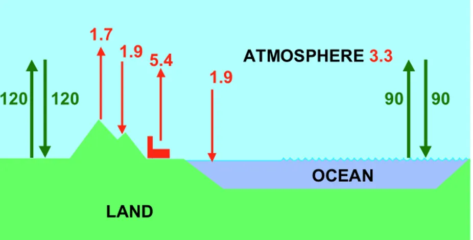
OCEAN LAND ATMOSPHERE 90 90 120 120 5.4 1.7 1.9 1.9 3.3
Figure 3.2: Visualisation of the carbon fluxes between land, atmosphere and ocean. The green arrows represent natural fluxes in equilibrium. The red arrows represent the carbon fluxes as a consequence of anthropogenic disturbance. The values, valid for the 1980s) (see Table 3.1) are taken from IPCC (2001).
IPCC SRES projections
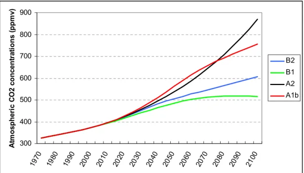
Figure 3.3 shows how the oceanic fluxes follow the net atmospheric fluxes: a large increase in the net flux because of increasing energy emissions and deforestation fluxes (A2) is partly
compensated by an increased uptake flux of carbon into the ocean. On the other hand, the figure shows a lower oceanic uptake in the B1 world, where the net flux declines because of a decreasing population focused on sustainable development. The resulting CO2 concentration
profiles are depicted in Figure 3.4.
-10 -5 0 5 10 15 20 1970 1980 1990 2000 2010 2020 2030 2040 2050 2060 2070 2080 2090 2100 C ar bon f lux es ( G t C /y r) Oceans - B2 Net flux - B2 Oceans - B1 Net flux - B1 Oceans - A2 Net flux - A2 Oceans - A1b Net flux - A1b
Figure 3.3: Two carbon fluxes for each SRES scenario (IPCC, 2000): the oceanic uptake and the net flux in Gt C per year. Results are taken from IMAGE team (2001a).
300 400 500 600 700 800 900 1970 1980 1990 2000 2010 2020 2030 2040 2050 2060 2070 2080 2090 2100 A tm o sphe ri c C O 2 c onc en tr at ions ( ppm v) B2 B1 A2 A1b
Figure 3.4: The atmospheric CO2 concentrations for the SRES scenarios (IPCC, 2000) as
3.2 Atmospheric Chemistry Model (ACM)
The Atmospheric Chemistry Model (ACM) calculates the global-mean atmospheric concentrations of the most important non-CO2 greenhouse gases and ozone precursors. All
the model input and output variables of ACM are listed below:
Model input - Land-use and natural emissions of CH4, N2O, NOx, CO and NMVOC
(from TES)
- Energy and industry emissions of CH4, N2O, NOx, CO, NMVOC and the
halocarbons (from EIS)
Model output - Concentrations of CH4, N2O, tropospheric ozone and halocarbons (used
as input in UDCM)
- Concentrations of CO and the OH-radical - Chemical and atmospheric lifetime of CH4
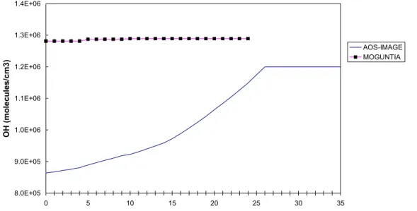
The first version of ACM was developed by Krol and Van der Woerd (1994). An extensive sensitivity analysis with the model, as described in Eickhout (1999), showed that ACM did not give good results in more extreme scenarios. Figure 3.5 shows that the ACM versions in IMAGE 2.0 and 2.1 even needed a ceiling for the OH concentrations; otherwise, the OH concentrations would increase too fast. The reason for this very reactive result of IMAGE 2.0/2.1 lies within a chain of chemical reactions of NOx, CO and CH4 that is too interlinked
and so leads to too much mutual strengthening. For further information on the shortcomings of AOS-IMAGE 2.0/2.1, the reader is referred to Eickhout (1999). The new version of AOS is explained below. 8.0E+05 9.0E+05 1.0E+06 1.1E+06 1.2E+06 1.3E+06 1.4E+06 0 5 10 15 20 25 30 35 OH ( m o lec u le s/ cm 3) AOS-IMAGE MOGUNTIA
Figure 3.5: Comparison of a sensitivity run by AOS-IMAGE 2.0/2.1 and the three-dimensional global chemistry model, MOGUNTIA (introduced by Zimmerman, 1988 and further developed by The, 1997). In this sensitivity run the CH4 and CO emissions are kept
constant, and the emissions of NOx and NMVOC are increased by 1% per year for over a
period of 35 years. The different absolute values in the first year are introduced by different model settings. For further information on these sensitivity runs, the reader is referred to Eickhout (1999).
Methodology
Except for N2O and the CFCs, the non-CO2 greenhouse gases are not as inert as CO2.
Consequently, the different gases are closely linked to each other and the change in concentration of one gas influences the change in concentration of another gas. This
dependency is seeking an elegant means to model the intermolecular dependencies and, at the same time, keep computation time within acceptable limits. The modelling methodology is explained below.
CH4, N2O and halocarbons
The emissions of the greenhouse gas and its subsequent removal from the atmosphere determine the concentration. The lifetime of a greenhouse gas indicates the efficiency of the removal process and is a measure of the time that passes before an emission pulse is removed from the atmosphere. For methane (CH4), nitrogenous oxide (N2O) and the halocarbons
(including SF6), the rate of removal is linearly dependent on the concentration of the
compound, and is derived by multiplying the concentration by the lifetime factor, as adopted in most current IPCC simple climate models (Harvey et al., 1997). The rate of change for the concentration is then expressed as:
[
]
[
]
GHG GHG GHG GHG E cv t GHG t -× = D D (3.6)where ∆GHG is the atmospheric concentration of greenhouse gas GHG, EGHG the total
emissions, tGHG the atmospheric exponential decay time or lifetime (yr) and cvGHG a
mass-to-concentration conversion factor. The lifetime of nitrous dioxide (N2O) and most halocarbons
(except for the partial chlorinated halocarbons: HCFCs, HFCs and CH3CCl3; see Table 3.2) is
assumed to be constant because of the inertness of these gases.
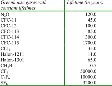
Table 3.2: Atmospheric lifetimes of the most important greenhouse gases assumed to be inert in the troposphere (constant lifetime), as adopted in IMAGE 2.2. Source: IPCC, 2001
Greenhouse gases with constant lifetimes
Lifetime (in years)
N2O 120.0 CFC-11 45.0 CFC-12 100.0 CFC-113 85.0 CFC-114 300.0 CFC-115 1700.0 CCl4 35.0 Halon-1211 11.0 Halon-1301 65.0 CH3Br 0.7 CF4 50000.0 C2F6 10000.0 SF6 3200.0
Because of the reactivity of the greenhouse gases, CH4, HCFCs, HFCs and CH3CCl3 with the
OH radical, the atmospheric lifetimes of these gases cannot be assumed to be constant. The OH abundance for these compounds is also taken into account. Hence, the atmospheric lifetime in Equation 3.7 is calculated as:
loss soil ric stratosphe chemical GHG = t + t + t -t 1 1 1 1 (3.7)
where: τGHG = atmospheric lifetime of greenhouse gas GHG (i.e. CH4, HCFCs,
HFCs and CH3CCl3: in years);
τchemical = chemical lifetime of the same greenhouse gas (in years);
τstratospheric = lifetime due to loss to stratosphere (in years);
τsoil-loss = lifetime due to loss to biosphere (soil; in years).
The lifetimes due to losses to the stratosphere and the biosphere are assumed constant. The chemical lifetime of these greenhouse gases is determined by the reaction rate for the oxidation by OH radicals (assuming a one-order reaction):
] [ * 1 OH kGHG OH chemical + = t (3.8) with:
kGHG+OH = reaction rate (cm3 per year)
[OH] = OH concentration (molecules per cm3)
Hence, the abundance of the OH radical in the troposphere determines the chemical lifetime of the reactive tracers, and therefore the atmospheric lifetime (Equation 3.7) and the
atmospheric concentration (Equation 3.6).
The OH radical plays an important role in the tropospheric chemistry because of its reactivity. Equation 3.9 shows that the OH radical is involved in a set of reactions with, in this case, methane and CO. Methane can be replaced by all other non-methane volatile organic compounds (NMVOCs).
× ® + × + × ® × + × ® + × × + ® × + 2 3 2 3 2 3 4 2 2 2 O CH O CH O H CH OH CH HO O H H CO OH CO (3.9)
Furthermore, the presence of NOx determines whether more radicals are formed or depleted.
In the absence of NOx, fewer radicals can be formed and less tropospheric ozone depleted
(Equation 3.10); in the presence of NOx more radicals and tropospheric ozone can be formed
(Equation 3.11). O H or OH CH O OH HO or O CH OH or O CH O O HO or O CH 2 3 2 2 2 3 3 2 3 2 2 3 2 + ® × + × × × × + ® + × × (3.10)
(
)
3 2 2 3 2 2 2 3 410 O O O O NO nm h NO OH or O CH NO NO HO or O CH ® + × × + ® £ + × × + ® + × × l n (3.11)This complex reaction scheme represents only a small part of the many reactions with OH occurring in the troposphere. In IMAGE 2.2, the OH abundance is calculated with use of sensitivity coefficients for reactions of OH with CH4, CO, NOx and NMVOC. This approach
is based on the OxComp experiment, developed to calculate the atmospheric concentrations of the most important reactive gases, given the SRES scenarios (IPCC, 2001). In this approach, simple parameterisations are determined by re-simulating the results of complex three-dimensional atmospheric chemistry models of one SRES run. Although the resulting parameterisation of the complex tropospheric chemistry has been very simplified (see
Equation 3.12), it gives a good idea of the concentration change in the OH radical expected in the future. However, note that the approach neglects the possible impact of climate change on the tropospheric chemistry.
[ ]
[
]
NO NO CO CO NMVOC NMVOC CH CH R E R E R E R OH x x ×D + ×D + ×D + D × = D 4 ln ln 4 (3.12)where Rgas stands for the sensitivity coefficient of each reactive gas (see Table 3.3).
Table 3.3: Sensitivity coefficients to determine the change of OH abundance and tropospheric ozone concentration, as shown in Equations 3.12 and 3.14.
Sensitivity coefficient In relation to the OH radical
(Equation 3.12) In relation to tropospheric ozone (Equation 3.14) RCH4 -0.32 6.7 RNOx 0.0042 0.17 RCO -0.000105 0.0014 RNMVOC -0.000315 0.0042
Note: Values are based on the OxComp experiment (IPCC, 2001).
This sensitivity coefficient determines the OH abundance, depending on the increase in the four mentioned reactive gases. Table 3.3 shows the OH abundance to decline by 0.32% for every 1% increase in CH4. This sensitivity coefficient is also called the chemical feedback
parameter.
With the calculated OH abundance from Equation 3.12, the concentrations of CH4, HCFCs,
HFCs and CH3CCl3 can be calculated. For these calculations, the lifetimes due to losses to
the stratosphere and biosphere (Equation 3.7) plus the reaction rate (Equation 3.8) need to be known. In Table 3.4 these fixed values are summarised (based on Krol and Van der Woerd, 1994 and IPCC, 2001).
Table 3.4: Reaction rates and transport losses of greenhouse gases that react with the OH radical (CH4, HCFCs, HFCs and CH3CCl3) and taken into account by IMAGE 2.2.
Greenhouse gas taken into account by IMAGE 2.2
Reaction rate of the
oxidation by OH (in cm3/yr)
Transport losses to stratosphere and biosphere ( yr-1) CH4 1.274·10-7 0.0063 CH3CCl3 1.781·10-7 0.0213 CH3Cl 9.101·10-7 0.02 HCFC-22 8.482·10-8 0.0042 HCFC-123 8.150·10-7 0.0213 HCFC-124 1.985·10-7 0.0078 HCFC-141b 1.144·10-7 0.0132 HCFC-142b 5.773·10-8 0.0046 HCFC-225ca 1.683·10-7 0.0083 HFC-23 4.640·10-9 0.0 HFC-32 1.930·10-7 0.0 HFC-43-10-mee 9.236·10-8 0.0 HFC-125 3.552·10-8 0.0 HFC-134a 9.236·10-8 0.0 HFC-143a 2.110·10-8 0.0 HFC-152a 8.044·10-7 0.0 HFC-227ea 2.830·10-8 0.0 HFC-236fa 4.640·10-9 0.0 HFC-245ca 1.660·10-7 0.0
Note: For CH4, the respective transport losses to stratosphere and biosphere were
determined at 1/120 and 1/160. These values are taken from Krol and Van der Woerd (1994) and IPCC (2001).
Tropospheric ozone (O3)
As already shown, the tropospheric ozone concentration is very much connected to the OH abundance. Some further reactions are given in the following scheme:
× ® + × ® + × + × ® £ + OH O H O O O O O O nm h O 2 ) 310 ( 2 3 2 2 3 n l (3.13)
Hence, the determination of tropospheric ozone is very similar to the determination of the OH abundance. Again, this approach is based on the OxComp experiment in IPCC (2001). See Table 3.3 for the values in Equation 3.14.
[
]
[
]
NO NO CO CO NMVOC NMVOC CH CH R E R E R E R O trop x x ×D + ×D + ×D + D × = D 4 3 ln . ln 4 (3.14)In this way ACM is still globally averaged, but the shortcomings of AOS-IMAGE 2.0/2.1 (Eickhout, 1999) are removed.
The determination of the CO concentration has not changed since Krol and Van der Woerd (1994).
Calibration
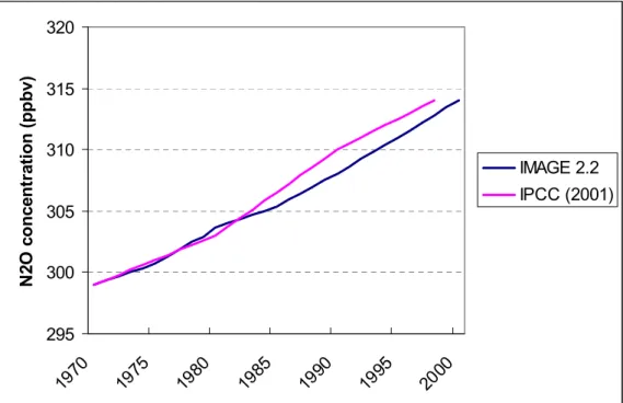
Given the historical emissions from EIS and the calibrated emissions from TES, ACM is compared with historical data for N2O (Figure 3.6) and CH4 (Figure 3.7). Until 1990 IMAGE
2.2 was very capable of following the historical data.
For methane (CH4) IMAGE follows the measured data very well until 1990. However, after
1990 some differences are very clear. For CH4 the decrease of methane in the 1990s cannot
be reproduced by IMAGE 2.2. However, the decline in the methane yearly growth rate after 1991 has been topic of great discussion. One of the hypotheses is that the Pinatubo eruption in 1991 caused a decrease in stratospheric ozone and therefore an increase in UV in the troposphere. An increase in UV would increase the OH abundance and therefore the decrease in methane. Since IMAGE 2.2 uses constant vulcano emissions, this extreme event cannot be reproduced by ACM. 295 300 305 310 315 320 1970 1975 1980 1985 1990 1995 2000 N 2O co n cen tr at io n ( p p b v) IMAGE 2.2 IPCC (2001)
Figure 3.6: Historical N2O concentration in ppbv; IMAGE 2.2 results compared with data
1.3 1.4 1.5 1.6 1.7 1.8 1.9 1970 1975 1980 1985 1990 1995 2000 C H 4 c oncent rat ion ( ppm v) IPCC (2001) IMAGE 2.2
Figure 3.7: Historical CH4 concentration in ppmv; IMAGE 2.2 results compared with data
(IPCC, 2001).
IPCC SRES projections
Figures 3.8 and 3.9 show the SRES projections as implemented by IMAGE 2.2 (IMAGE team, 2001a). Again the A2 and B1 scenario span up the SRES range by the end of the 21st century. 250 300 350 400 450 500 1970 1985 2000 2015 2030 2045 2060 2075 2090 A tmos phe ri c N 2O c onc en tr at ions (ppbv ) B2 B1 A2 A1b
Figure 3.8: Atmospheric concentrations for N2O for the SRES scenarios (IPCC, 2000) as
1 1.5 2 2.5 3 3.5 4 4.5 1970 1980 1990 2000 2010 2020 2030 2040 2050 2060 2070 2080 2090 2100 A tm o sp h er ic C H 4 co n cen tr at io n s ( p p m v) B2 B1 A2 A1b
Figure 3.9: Atmospheric concentrations for CH4 for the SRES scenarios (IPCC, 2000) as
4. Modelling radiative forcing
Increased concentrations of greenhouse gases in the atmosphere lead to a change in radiative forcing, a measure of the extra energy input to the surface-troposphere system. This increased radiative forcing leads to an increase in the global-mean surface temperature. The radiative forcing calculations are fully based on the latest scientific literature as assessed in the TAR (IPCC, 2001). This chapter presents the methodology, calibration and the SRES projections of the radiative forcing calculations by IMAGE 2.2, which is part of the Upwelling-Diffusion Climate Model (UDCM; see Figure 2.1).
4.1 Methodology
The methodology for determining the radiative forcings is given outlined in his section. The input and output of this AOS is given in the textbox below.
Model input - Atmospheric concentrations of the most important greenhouse gases (CO2, CH4, N2O, tropospheric O3, CFCs, HCFCs, PFCs, Halon-1211, Halon-1301, CH3Br, SF6, CH3CCl3 and CH3Cl (modelled in OCM and ACM; see Chapter 3).
- Energy and land-use emissions of SO2 (modelled in EIS and TES).
Model output - Changes in radiative forcing for CO2, CH4, N2O, tropospheric O3, stratospheric O3, CFCs, HCFCs, PFCs, Halon-1211, Halon-1301, CH3Br, SF6, CH3CCl3, CH3Cl, stratospheric water vapour and a number of tropopsheric aerosols (used as input for UDCM).
CO2
The radiative forcing of carbon dioxide is calculated as:
[ ]
[ ]
÷÷ø ö ç ç è æ × = D 0 2 2 2 , 5.325 ln t t t CO CO CO Q (4.1)where t0 is 1765, the year of initialisation in IMAGE 2.2 (see section 3.1). The pre-industrial
concentration of CO2 is assumed to be 278 ppmv.
The value, 5.325, is based on the fact that doubling of the CO2 concentration will lead to an
increased forcing of 3.7 Wm-2. This is in line with the assumed value given by IPCC (2001). CH4 and N2O
As the concentration of a greenhouse gas increases, the forcing will gradually ‘saturate’ into certain absorption bands. An additional unit increase in concentration will gradually have a relatively smaller impact on radiative forcing. At present-day concentrations, the saturation effect is greatest for CO2 and somewhat less for CH4 and N2O.
Additionally, some greenhouse gases absorb radiation in each other’s frequency domains. This ‘overlap effect’ is especially relevant for CH4 and N2O. Increases in CH4 concentration
decrease the efficiency of N2O absorption and vice versa. IMAGE 2.2 uses the following
[
]
[
]
(
)
(
)
(
)
(
)
(
)
÷÷ ÷ ÷ ÷ ÷ ÷ ø ö çç ç ç ç ç ç è æ ú ú û ù ê ê ë é × × + × × + × -ú ú û ù ê ê ë é × × + × × + × -× = D 52 . 1 2 4 4 75 . 0 2 4 52 . 1 2 4 4 75 . 0 2 4 4 4 , 0 0 0 0 0 0 0 0 4 ] [ ] [ ] [ ] [ ] [ 1 ln 47 . 0 ] [ ] [ ] [ ] [ ] [ 1 ln 47 . 0 036 . 0 t t t t t t t t t t t t t CH O N CH CH b O N CH a O N CH CH b O N CH a CH CH Q (4.2)for the change into radiative forcing of methane, and:
[
]
[
]
(
)
(
)
(
)
(
)
(
)
÷÷ ÷ ÷ ÷ ÷ ÷ ø ö çç ç ç ç ç ç è æ ú ú û ù ê ê ë é × × + × × + × -ú ú û ù ê ê ë é × × + × × + × -× = D 52 . 1 2 4 4 75 . 0 2 4 52 . 1 2 4 4 75 . 0 2 4 2 2 , 0 0 0 0 0 0 0 0 0 2 ] [ ] [ ] [ ] [ ] [ 1 ln 47 . 0 ] [ ] [ ] [ ] [ ] [ 1 ln 47 . 0 12 . 0 t t t t t t t t t t t t t O N O N CH CH b O N CH a O N CH CH b O N CH a O N O N Q (4.3)for the change into radiative forcing of nitrous oxide. The pre-industrial concentrations
0
]
[CH4 t and [N2O]t0 are assumed to be 700 and 270 ppbv, respectively (IPCC, 2001). The values a and b are 2.01 x 10⁻⁵ and 5.31 x 10⁻¹⁵, respectively.
Tropospheric ozone (O3), halocarbons and SF6
These greenhouse gases are calculated by using the tropospheric concentrations (calculated in ACM; see section 3.2) multiplied by the so-called radiative efficiency coefficients taken from IPCC (2001). Table 4.1 contains the radiative efficiency coefficients used in IMAGE 2.2. Stratospheric ozone
Chlorinated and brominated halocarbons can lead to significant indirect forcing by the depletion of stratospheric ozone. This indirect forcing effect of some of the halocarbons is taken into account in IMAGE 2.2. However, the indirect effect of increasing UV field in the troposphere is not taken into account in IMAGE 2.2. An increase in UV because of less stratospheric ozone leads to an increase in OH and hence, an increased atmospheric decay of other greenhouse gases (methane). This effect is very difficult to quantify, especially since the ozone depletion is highly dependent on the altitude profile of the ozone loss. Therefore, only the forcing due to loss of stratospheric ozone is quantified in IMAGE 2.2. The following equation is used for this effect (Harvey et al., 1997):
{
}
(
)
(
)
[
å
× +å
]
´ -= DQstratO t NCli Cit NBriCi,t 7 . 1 , , . 3 0.001 0.000552 3.048 (4.4)where Ci is the concentration in pptv of chlorinated or brominated halocarbon i and NCli and
NBri are the number of chlorine or bromine atoms in compound i. In Table 4.1, the number of
chlorine or bromine atoms are summed for the ozone-depleting compounds taken into account.
Stratospheric water vapour
The oxidation of methane produces water vapour that can contribute significantly to changes in stratospheric water vapour, which in itself, also leads to a radiative forcing. However, so far not much is known about the processes contributing to this forcing. In IMAGE 2.2, the indirect effect of methane oxidation is taken into account by the following equation (Harvey et al., 1997):
[
]
[
]
(
4 4 1765)
, , . 2 0.05 Q 4 0.05 0.036 CH CH QstratHOt = ×D CH directt = × × t -D - (4.5)Direct radiative forcing of tropospheric aerosols
In IMAGE 2.2, only the direct effects of the sulphate, fossil fuel black carbon, fossil fuel organic carbon and biomass burning aerosols are taken into account. Other tropospheric aerosols such as mineral dust aerosols and nitrate aerosols are not considered. IPCC (2001) estimates the effect of mineral dust aerosols from –0.60 to 0.40 W/m2. Given the lack of scientific information on nitrate aerosols “best estimates” are not given.
The direct effect of aerosols is caused by scattering and absorbing short-wave and long-wave radiation with a resulting perturbation of the energy budget of the Earth/atmospheric system. In simple climate models (SCMs) the direct component of the forcing is assumed to vary linearly with concentration and hence with emissions. In an equation for the effect of sulphate aerosols (Harvey et al., 1997):
1990 , 1990 , , , 4 2 2 4 SO direct SO t SO t direct SO Q emis emis Q - = ×D -D (4.6)
where forcing in 1990 is assumed to be -0.3 W/m2. Note that only the anthropogenic
emissions due to energy use and industrial activities are considered in this equation. The 1990 emissions within IMAGE 2.2, are assumed to be 71.6 Tg S (Olivier et al., 1996).
For fossil fuel, black and organic carbon aerosols, the same approach as for sulphate aerosols is chosen, since these aerosols are also formed due to anthropogenic energy and industrial emissions. Note that soot decreases the reflection and thus, increases the absorption of solar radiation. The 1990 level of the combination of black and organic carbons is assumed to be 0.1 W/m2 (IPCC, 2001).
The same approach is used again for biomass burning aerosols. However, scaling for these aerosols is performed using the change in SO2 emissions due to land-use change. In 1990, the
land-use emissions are 1.75 Tg S (IMAGE team, 2001a), while the forcing in 1990 due to biomass burning aerosols is assumed to be –0.2 W/m2 (IPCC, 2001).
Indirect radiative forcing of tropospheric aerosols
Aerosols serve both as cloud condensation and ice nuclei. As a result, the aerosols change the microphysics, the radiative properties and the lifetime of clouds, and hence, change the cloud albedo and amount. This effect is called the indirect radiative forcing caused by aerosols. Moreover, there are two indirect effects to distinguish: 1) an increase in aerosols, causing an increase in droplet concentration, and 2) the reduction in cloud droplet size, affecting the precipitation efficiency and tending to increase the liquid water content, the cloud lifetime and the cloud thickness (IPCC, 2001). Because of the many uncertainties, it is very difficult to quantify these indirect effects. A few factors that may contribute to this uncertainty are:
· that pre-industrial sulphate varies by a factor of just over 2;
· that the variance in the industrial sulphate concentrations is about 50%; · that the parameterizations of relating droplet number concentration to aerosol
concentration are very uncertain;
· that changes in the vertical distribution of the aerosol will affect the indirect forcing because of changes in its spatial relationship to cloud (IPCC, 2001).
Table 4.1: Radiative efficiency coefficients in IMAGE 2.2 based on IPCC (2001)3) Chemical compound Radiative efficiency coefficient
(in W*m-2*ppbv-1)
Number of chlorine or
bromine atoms per compound
Tropospheric ozone1) 0.0422) 0 CFC-11 0.25 3 CFC-12 0.32 2 CFC-113 0.30 3 CFC-114 0.31 2 CFC-115 0.18 1 CCl4 0.13 4 CH3CCl3 0.06 3 CH3Cl1) 0.01 1 HCFC-22 0.20 1 HCFC-123 0.20 2 HCFC-124 0.22 1 HCFC-141b 0.14 2 HCFC-142b 0.20 1 HCFC-225ca 0.27 2 HFC-23 0.16 0 HFC-32 0.09 0 HFC-43-10-mee 0.40 0 HFC-125 0.23 0 HFC-134a 0.15 0 HFC-143a 0.13 0 HFC-152a 0.09 0 HFC-227ea 0.30 0 HFC-236fa 0.28 0 HFC-245ca 0.23 0 Halon-1211 0.30 1 Halon-1301 0.32 1 CH3Br1) 0.01 14) CF41) 0.08 0 C2F6 0.26 0 SF6 0.52 0
1) The pre-industrial concentration of natural occurring greenhouse gases is subtracted before the multiplication by the radiative efficiency coefficient to obtain the radiative forcing compared to pre-industrial times. Pre-pre-industrial concentrations are 25.0 DU (Dobson Unit) for tropospheric ozone, 600 ppbv for CH3Cl, 4.1ppbv for CH3Br and 40ppbv for CF4.
2) The unit of the radiative efficiency coefficient for ozone is W*m-2*DU-1.
3) The values for the halocarbons and SF6 are taken from Table 6.7 and for O3 from Table 6.3.
Within IMAGE 2.2, only the first indirect effect of sulphate aerosols is taken into account. Indirect radiative forcings by carbonaceous aerosols, mineral dust aerosols and gas-phase nitric acid are rarely assessed. Hence, IMAGE 2.2 cannot quantify these effects. For the indirect effect of sulphate aerosols, IMAGE 2.2 uses the equation according to Harvey et al. (1997): 1990 , 1990 , , , 4 2 2 2 2 4 1 log 1 log indirect SO nat SO SO nat SO t SO t indirect SO Q emis emis emis emis Q -- ×D ÷ ø ö ç è æ + ÷ ø ö ç è æ + = D (4.7)
where the indirect forcing in 1990 is assumed to be –0.8 W/m2. The natural emissions are mainly volcanoes and dimethyl sulphide (by oceans, land biota and soils). These emissions are difficult to quantify. IMAGE 2.2 uses a constant amount of 34.4 Tg S per year and well within the range of the IPCC (2001): 18-62 Tg S per year.
Note that because of the logarithm dependence of the indirect effect, the direct effect of sulphate aerosols becomes relatively larger when the sulphate aerosol loading increases. Forcings not taken into account
Besides the forcings already mentioned, the following forcings are not taken into account either by IMAGE 2.2: the forcing by stratospheric aerosols, and the forcing due to both surface albedo effect and solar activity. The forcing by stratospheric aerosols is mainly caused by volcanic eruptions. Although these effects can have large impacts on the balance (e.g. up to –3 ± 0.6 W/m2 due of the eruption of the Mt. Pinatubo in 1991), the lack of a reliable record of episodic volcanic events, especially before the 1960s, makes it hard to project future effects.
Land-use changes can cause changes in the land surface albedo as well. However, the responses differ very much per latitudinal band and per landcover type (the albedo of a cultivated field is affected more by a given snowfall than the albedo of an evergreen forest). Future quantification of this effect is not given in IMAGE 2.2, although IMAGE 2.2 provides an extensive amount of data for future land cover.
Total solar irradiance (TSI) is another factor with many uncertainties. The most important uncertainties, posed in IPCC (2001), are:
· what is the absolute value of the TSI? (only records of the last two decades are available; with many disagreements);
· from what other proxy measure of solar output can the historical variation be deduced? (sunspot numbers, solar diameter etceteras);
· how much impact do variations in stratospheric composition and thermal structure
resulting from ultraviolet irradiance have on tropospheric climate? (increase in downward infrared flux by heating the stratosphere; effects of changing ozone concentrations due to changing irradiance);
· how important is the correlation between total cloud cover and cosmic ray fluxes? (are galactic cosmic rays less able to reach the Earth when the sun is more active because of fluctuations in the sun’s magnetic field?).
Because of the extent of the uncertainties in the above-mentioned cases, IMAGE 2.2 does not take these possible effects into account. Taking the change in global and annual mean
radiative forcing from 1750 allows IPCC (2001) to give the following estimates for possible mechanisms not taken into account by IMAGE 2.2:
Direct mineral dust aerosols: -0.60 to +0.40 W/m2; Aviation-induced cirrus: 0 to +0.04 W/m2; Aviation-induced contrails: +0.02 W/m2; Land use (albedo): -0.20 W/m2;
Solar: +0.30 W/m2.
Note that the choice of the year 1750 is crucial for the estimate of the solar effect. A choice of 1700 would give values about twice as large. Given these values and the different
uncertainties, it would seem justified to disregard these effects in IMAGE 2.2 until more is known.
4.2 Calibration
The global and annual mean radiative forcing from 1765 to the early 1990s is projected in Figure 4.1 (the results for 1995 are used for IMAGE 2.2). This figure shows that IMAGE 2.2 returns results for its historical period (1765-1995) that are well in line with the latest
scientific information available (IPCC, 2001). The slightly higher value of IMAGE 2.2 for the direct sulphate aerosol forcing (less negative) is the main result of a starting point of -0.3 W/m2 (Harvey et al., 1997), but is also caused by the decrease in sulphur emissions in China, based on emission data up to 1995.
-2 -1.5 -1 -0.5 0 0.5 1 1.5 2 2.5 3 Wel l-mixed GHG Trop . Ozo ne Stra t. Ozon e Stra t. W ater vap our Dire ct sulp hate aer osol s Indi rect sulph ate aero sols Dire ct FF aero sols (BC & O C) Dire ct b iomas s bu rnin g ae roso ls G loba l m e a n r a d ia tiv e f o rc ing (W /m 2) IPCC IMAGE 2.2
Figure 4.1: Global and annual mean radiative forcing from 1750 to present according IPCC (2001) and from 1765 to 1995 according IMAGE 2.2 (IMAGE team, 2001a). Only the effects taken into account by IMAGE 2.2 are visualised.
The projected changes in radiative forcing are used as input for the Upwelling-Diffusion Climate model (UDCM) of IMAGE 2.2.
4.3 IPCC SRES projections -2 0 2 4 6 8 10 1995 A1b-2100 B1-2100 A2-2100 B2-2100 R adi at iv e fo rc ing ( in W /m 2) Indirect Sulphate Direct Sulphate Trop. O3 N2O CH4 CO2
Figure 4.2: Radiative forcing since 1765 for the SRES scenarios according IMAGE 2.2 (IMAGE team, 2001a) for CO2, CH4, N2O, tropospheric O3 and direct and indirect sulphate
aerosols. The values for 1995 are depicted as well.
Figure 4.2 shows the radiative projections for 2100 for the four different SRES scenarios. Clearly, the sustainable scenario B1 has low sulphate forcings because of policies against SO2 emissions. The differences in the greenhouse gas concentrations, shown in Chapter 3,
5. Modelling the global-mean temperature change
In IMAGE 2.2 the reaction of the climate system to increased forcing is calculated by a global-mean, upwelling-diffusion, energy-balance model. Section 5.1 describes the methodology of the model. Again, in the following two sections, much attention is paid to calibration of the model and the implementation of the SRES scenarios.
5.1 Methodology
In this section, the methodology of the upwelling-diffusion climate model (UDCM; see Figure 2.1) is explained in further detail. The reader is also referred to Appendix A for further mathematical details. The energy-balance model was introduced in 1985 by Wigley and Schlesinger (1985), and Harvey and Schneider (1985). The elaboration on this model and the inclusion of upwelling-diffusion characteristics was introduced by Wigley and Raper (1987) as the MAGICC model. The latest version of MAGICC (Version 2.4) described here is implemented in IMAGE 2.2. MAGICC is also described in its most recent form in Raper et al. (1996) and Hulme et al. (2000).
The energy-balance model
The model consists of an atmosphere box, coupled to northern and southern hemisphere land and ocean boxes (see Figure 5.1). The two ocean boxes are each divided into 40 layers, with a mixed layer on top that absorbs the energy of solar radiation. Above land, no energy is
assumed to be adsorbed. The energy balance of the climate system can be described as: F
T Q= D a +D
D l (5.1)
where ∆Q is the global increase in radiative forcing (in W×m-2; see Chapter 4) and ∆F the net
heat flux into the ocean (in W×m-2; both averaged over the entire world area). The term λ∆T a
is the change in the rate of heat loss to space from the climate system. The feedback parameter, λ, is the inverse of the climate sensitivity (in °C-1): the long-term (equilibrium)
annual and global-mean surface-air temperature increase for a doubling of the CO2 concentration since pre-industrial times is denoted by DT2´ (IPCC, 1996). This value is a
very important factor for determining the reaction of the climate system (in terms of temperature change) as a response to changes in the CO2 concentration. In section 5.2, we
elaborate further on the uncertainties in the climate sensitivity and its consequences for climate impacts.
Figure 5.1 The boxes distinguished in the Upwelling-Diffusion Climate Model (Harvey et al., 1997).
Hence, the radiative forcing is partitioned between increased heat loss to space and additional uptake of heat by the climate system (Raper et al., 2001). The absorbed heat is exchanged between the four boxes (determined by kLO and kNS; the land-ocean and northern-southern
hemisphere exchange coefficient, respectively). On time scales relevant to climate change, the changes in the atmosphere may be assumed to be in equilibrium with the underlying oceanic mixed layer:
F T Q dt T d C O a m =D - D -D D l 1 , (5.2)
where d∆TO,1 is the temperature change of the oceanic mixed layer and Cm the effective bulk
heat capacity of the oceanic mixed layer (Wigley and Schlesinger, 1985).
The four complete equations (including the exchange coefficients land-ocean and the two hemispheres) can be derived from Equation 5.2. The effective bulk heat capacity is expressed as a product of the density of seawater (ρ), the specific heat capacity of water (c) and the height of the oceanic mixed layer (hm). The four equations are: