Michel den Elzen
∗1and Malte Meinshausen
2 1National Institute for Public Health and the Environment (RIVM),Netherlands Environmental Assessment Agency, PO Box 1,3720 BA Bilthoven, The Netherlands, e-mail: michel.den.elzen@rivm.nl
2
Swiss Federal Institute of Technology (ETH Zurich), Environmental Science Department, Rämistrasse 101,CH-8092 Zurich, Switzerland, e-mail: malte.meinshausen@env.ethz.ch
Emission implications of long-term climate targets
Key words: multi-gas pathway, climate target∗
Tel.: +31-30-2743584; fax: +31-30-27424427; E-mail address: michel.den.Elzen@rivm.nl
Emission implications of long-term climate targets
Michel den Elzen
1and Malte Meinshausen
2 1National Institute for Public Health and the Environment (RIVM),Netherlands Environmental Assessment Agency, PO Box 1,3720 BA Bilthoven, The Netherlands, e-mail: michel.den.elzen@rivm.nl
2
Swiss Federal Institute of Technology (ETH Zurich), Environmental Science Department, Rämistrasse 101,CH-8092 Zurich, Switzerland, e-mail: malte.meinshausen@env.ethz.ch
Abstract
This paper presents a set of multi-gas emission pathways compatible with different levels of ambition of avoiding long-term climate change, expressed in terms of long-term temperature targets, such as the EU 2oC target, and the certainty of achieving these. Also the effect of different assumptions on the resulting emission pathways, such as different baselines, technological improvement rates, or delay of global action is analysed. For achieving the EU target with a certainty of more than 50%, greenhouse gas concentrations need to be stabilised at 450 CO2 equivalent or lower, requiring global emissions to peak within the next two decades, followed by substantial overall reductions by as much as 30 to 50% in 2050 compared to 1990 levels. The total emission reductions and the abatement costs strongly depend on the emissions growth in the baseline scenario and the further improvements of the abatement potential and reduction costs for all greenhouse gases in the future.
1. Introduction
The aim of this study is to explore allowable emissions levels of the set of the six greenhouse gases covered under the Kyoto Protocol on the long and short term compatible with any long-term climate policy targets to avoid dangerous climate change. In order to determine allowable levels of greenhouse gas emissions we have to back-calculate from acceptable levels of climate change to emissions. This is not simple. Not only is there the question to solve “what is an acceptable level of climate change (if any)?”, but also because there are major uncertainties in the cause-effect chain - the relationship between levels of greenhouse gas emissions and the impacts related to the human-induced climate change. Thus, we take a pragmatic route: The point of departure of our analysis will be the long-term climate targets of the European Union [1], i.e. a maximum temperature increase of 2oC over pre-industrial levels. It should be kept in mind though that, 2°C cannot be regarded as ‘safe’ as shown by many reviews of the scientific literature [2-4]. For example, the risk of heatwaves like the European heatwave of 2003 (and the resulting unusually large numbers of heat-related deaths) doubled due to human-induced climate change [5, 6].
We then develop multi-gas abatement pathways and analyze their associated risks to overshoot a climate target, such as 2°C [7, 8]. Such a risk assessment takes conceptually account of the main uncertainties in the climate system. Most studies on the implications of a multi-gas reduction strategy are of more recent date [see e.g. 9]. An important reason is that consistent information on
reduction potential for the non-CO2 gases has been lacking. Available studies exploring the impacts of including non-CO2 gases in the analysis of the Kyoto Protocol nevertheless find that major cost reductions can be obtained through the relatively cheap abatement options for some of the non-CO2 gases and the increase in flexibility [10, 9]. Multi-gas studies on long-term stabilization targets indicate similar conclusions (e.g. Tol [11], Manne and Richels [12], van Vuuren et al. [13], den Elzen et al. [14]), or indicate important advantages in terms of avoiding climate impacts [15-17]. Other studies have explored the methodological issues of a multi-gas approach, such as which type of climate targets (for instance, concentration or temperature targets), can best be set for such a diverse group of gases (see Manne and Richels [12], Richels et al. [18], Fuglestvedt et al. [19] and O'Neill [20]).
Obviously, it is much more complicated to define emission scenarios for stabilising CO2 equivalent concentrations than CO2 only, because these can be reached by various combinations of gasses, that also have different contributions to the radiate budget over time. So far there are roughly five ways of accounting the non-CO2 emissions, by (i) simple scenario assumptions (e.g IPCC Third Assessment Report using a common non-intervention scenario (SRES A1B) for non-CO2 emissions [21]); (ii) ‘scaling’, concentrations or radiative forcing are proportionally scaled with CO2, for example, about 23% of CO2 forcing as in Raper et al. [22]), or a certain CO2 equivalent concentration level like 100ppm, to be added to a CO2-concentration stabilisation target [23]; (iii) accounting for source-specific reduction potentials for all gases, as in the post-SRES scenarios [24, 25], (iv) differently elaborated ways based on cost-optimisation over
the greenhouse gas emissions [13] and/or over time [12] and (v) meta-approaches that make use of the multi-gas characteristics in existing scenarios derived by any of the previous approaches [26].
Here we focus on a cost-optimization variant, which closely reflects the political reality of pre-set caps on aggregated emissions and individual cost-optimising actors that decide in regard to the mix of reductions across the different greenhouse gases. The analysis focuses on two questions for climate-change policy-making:
1. What are emission pathways compatible with different levels of ambition of avoiding long-term climate change, expressed in terms of long-term temperature targets, such as the EU 2oC target, and the certainty of achieving these?
2. What is the effect of different assumptions, such as different baselines and technological improvement rates of abatement potential and costs on the emission pathways, and their resulting emissions reductions and abatement costs?
In the next section, the overall method is presented that has been used for this analysis of linking global emission pathways with climate targets. Section 3 presents the results of the analysis for various concentration stabilisation targets, and analyses the impact of some of the major uncertainties. Section 4 presents the global abatement costs. The final section draws up several conclusions.
2. Method for the development of
emission pathways with
cost-effective multi-gas mixes
In order to assess the emission implications of different stabilization levels, this study presents new multi-gas emission pathways for the scenario period 2000-2400, that were derived by a method for a cost-effective mitigation of emissions. This method calculates the cost-optimal mixes of greenhouse gas emission reductions for a given global emission pathway under a least costs approach. The emission pathway is determined iteratively to match prescribed climate targets of any level, as described in detail below. It should be kept in mind though that this approach does not derive cost-effective pathways over the whole scenario period per se, but focuses on a cost-effective split among different greenhouse gas reductions for given emission limitations on GWP-weighted and aggregated emissions. For example, based on the current model version with static cost assumptions, we cannot make definitive judgments on how a delay in global action will affect overall mitigation costs. However, the model framework allows very well analyzing the existing policy framework with preset caps on GWP-weighted overall emissions under the assumption of cost-minimizing national strategies. The emissions that
have been adapted to meet the pre-defined stabilization targets include those of all major greenhouse gases (fossil CO2, CH4, N2O, HFCs, PFCs, SF6), ozone precursors (VOC, CO, NOx) and sulphur aerosols (SO2).
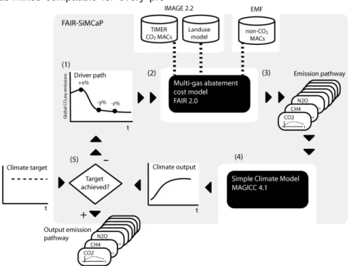
For our method we use the policy decision support tool FAIR 2.0 [27] in combination with another climate policy tool SiMCaP [26].
The FAIR (‘Framework to Assess International Regimes for the differentiation of commitments’) 2.0 model developed at the RIVM (the Netherlands) (www.rivm.nl/fair) is a policy decision-support-tool, which aims to assess the environmental and abatement costs implications of climate regimes for differentiation of post-2012 commitments [28, 27]. For the calculation of the emission pathways only the (multi-gas) abatement costs model of FAIR is used. This model distributes the difference between baseline and global emission pathway, over the different regions, gases and sources following a least-cost approach, taking full advantage of the flexible Kyoto Mechanisms (emissions trading) [14]. For this purpose, it makes use of (time-dependent) Marginal Abatement Cost (MAC) curves1 for the different regions, gases and sources (as described below). The FAIR model also uses baseline scenarios, i.e. potential greenhouse gas emissions in the absence of climate policies, from the integrated assessment model IMAGE2 and the energy model TIMER3.
The SiMCaP (‘Simple Model for Climate Policy Assessment’) model, developed at the ETH Zurich (Switzerland) (www.simcap.org), calculates global emission path-ways compatible with long-term climate targets [26]. The global climate calculations make use of the simple climate model MAGICC 4.1 [31-33]. More specifically, the pathfinder module of SiMCaP makes use of an iterative procedure to find emission paths that correspond to a predefined arbitrary climate target4.
The integration of both models, the ‘FAIRSiMCaP’ 1.0 model, enables to combine the strengths of both models, i.e.: (i) to calculate the cost-optimal mixes of greenhouse gases reductions for a global emissions profile under a least costs approach (FAIR); (ii) to find the global emissions profile that is compatible with any arbritary climate target (SiMCaP). The combination of both models
1 MAC curves that reflect the costs of abating the last ton of CO 2
-equivalent emissions and, in this way, describe the potential and costs of the different abatement options considered are used here.
2 The IMAGE 2.2 model is an integrated assessment model,
consisting of a set of integrated models that together describe important elements of the long-term dynamics of global environmental change, such as agriculture and energy use, atmospheric emissions of greenhouse gases and air pollutants, climate change, land-use change and environmental impacts [29].
3 The global energy model TIMER 1.0, as part IMAGE, describes
the primary and secondary demand and production of energy and the related emissions of greenhouse gasses and regional air pollutants [30].
4
For further details, e.g. assumptions in regard to natural forcing, see Meinshausen et al. [26].
allows to calculate global emission pathways with cost-effective gas-mixes compatible for every
pre-defined arbitrary climate target.
Figure 1 - FAIRSiMCaP model. The calculated global emission pathways were developed by using an iterative procedure as implemented in SiMCaP’s ‘pathfinder’ module using MAGICC to calculate the global climate indicators, the multi-gas abatement costs model of FAIR to allocate the emissions of the individual greenhouse gases and the IMAGE 2.2 and TIMER model for the baseline
emissions scenarios and the MAC curves (see text for details).
More specifically, the FAIRSiMCaP calculations consist of four steps (Figure 1):
1. Using the SiMCaP model to construct a driver parameterized global CO2-equivalent emission pathway, which is here defined by sections of linear decreasing or increasing emission reduction rates RI (initial 2010 value), RX, RY and RZ and years (X, Y and Z) at which the reduction rates change. This CO2-equivalent emission pathway5 includes all anthropogenic emissions of greenhouse gases, except the LUCF CO2 emissions (related to deforestation, and not sinks), as for those there are no MAC curves available. These LUCF CO2 emissions are described by the baseline scenario.
2. The abatement costs model of FAIR is used to allocate the global emissions reduction objective (except LUCF CO2 emissions), i.e. the difference between the baseline emissions and the global CO2-equivalent emission pathway (see Figure 2) of step 1 using a least-cost approach (cost-optimal implementation of reduction measures), for the period 2000-21006 over the six greenhouse gases using 100-year GWP indices and different sources
5 The CO
2-equivalent emissions are calculated using the emissions
of the six greenhouse gases combined with the 100 year Global Warming Potentials (GWPs) [34].
6 After 2100, the CO
2 eq reductions rates are applied to each
individual gas, except where non-reducible fractions (0.7) have been defined (N2O, CH4).
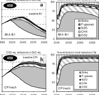
(e.g. for CO2: 12; CH4: 9; N2O: 7). Figure 2 shows the contribution of the different greenhouse gases in the global emissions reduction in order to reach, for this case, the 450ppm CO2-equivalent concentration level. It clearly shows that till 2025, there are potentially large incentives for sinks and non-CO2 abatement options (cheap options), so the non-CO2 reductions and sinks form a relatively large share in the total reductions. Later in the scenario period, the focus will be more on the CO2 reductions, and the contribution of most gases becomes more proportional to their share in baseline emissions. So in this way, the emission pathways of the different greenhouse gases are constructed.
Different sets of baseline- and time-dependent MAC curves for different emission sources are used here. Response curves from the TIMER model are used for the energy CO2 emissions [35], including technological developments, learning effects and system inertia7. For CO2 sinks the MAC curves of by the IMAGE model are used [36]. For non-CO2, exogenously determined MAC curves from EMF-21 [37-39] are used; these are based on detailed abatement options. As these curves were
7
These MAC curves will change in near future due to the implementation of new abatement options (e.g. hydrogen, biomass combined with carbon capture) and improvements of the present implementation of some abatement options (e.g. renewables, biofuels).
constructed for 2010 only, increases in the abatement potentials due to technology process and removal of implementation barriers are assumed. Here, a relatively conservative value of an increasing potential (at constant costs) for all other non-CO2 MAC curves of 0.4% per year is assumed [40, 36]. There are still some remaining agricultural emission sources of CH4 and N2O, where no MAC curves were available (e.g. for N2O agricultural waste burning, indirect fertilizer, animal waste and domestic sewage). As it is unlikely that these sources remain unabated under ambitious climate targets, we assumed a linear reduction towards a maximum of 35% compared to the baseline levels within a period of 30 years (2040). These MAC curves are used in the default calculations, and described in detail in van Vuuren et al. [35, 36].8
3. Using the simple climate model MAGICC 4.1, the greenhouse gas concentrations, and global temperature and sea level rise are calculated.
4. Within the iterative procedure of the SiMCaP model, the parameterizations of the CO2-equivalent emission pathway (step 1) are optimized (repeat step 1, 2 and 3) until the climate output and the prescribed target match sufficiently well.
These emission pathways have been developed for three underlying baseline scenarios:
1. IMA-B1: the IMAGE IPCC SRES B1 baseline [29] scenario with the LUCF CO2 emissions of this scenario and with the default MAC curves. This scenario assumes continuing globalization and economic growth, and a focus on the social and environmental aspects of life. The baseline emissions are given in Figure 2;
2. CPI: the Common POLES IMAGE (CPI) baseline [13, 36] scenario with the LUCF CO2 emissions of this scenario and with the default MAC curves. The CPI scenario assumes a continued process of globalisation, medium technology development and a strong dependence on fossil fuels. This corresponds to a medium-level emissions scenario when compared to the IPCC SRES emissions scenarios (Figure 2);
3. CPI-tech: the CPI baseline scenario with the LUCF CO2 emissions of the IMA-B1 scenario (less
8 The information on non-CO
2 abatement options and their costs
have been inventoried for EMF-21 for mainly 2010, over a limited cost range of 0 to 200 US$/tCeq and not all sources. We have assumed a certain increase in the reduction potential and costs as a result of technological development and the reduction of implementation barriers. The rate, at which these trends will evolve, however, is highly uncertain. Under the current implementation the cheap parts of the non-CO2 MACs tend to get exhausted before 2050 (Figure 2). This is
reflected in the rapid drop in the share of the non-CO2 gases in total
reductions over time. It will be crucial to extend research on non-CO2
emission reduction options beyond 2010 and on the sources, where no MAC curves are available. The presented results of this study may therefore change due to ongoing research in this area.
deforestation) and with MAC curves assuming additional technological improvements9.
CO2 -eq . emissio ns in Gt C-eq
0 5 10 15 2 0 2 5 19 9 5 2 0 2 0 2 0 4 5 2 0 70 2 0 9 5 IM A -B 1 450 b aseline B 1
%-co nt rib ut io n t o t al red uct io n (%)
0 2 5 50 75 10 0 2 0 10 2 0 3 5 2 0 6 0 2 0 8 5 Sinks F-gasses N 2O C H 4 C O2 IM A -B 1
CO2 -eq . emissio ns in Gt C-eq
0 5 10 15 2 0 2 5 19 9 5 2 0 2 0 2 0 4 5 2 0 70 2 0 9 5 450 C P I-tech b aseline CPI
%-co nt rib ut io n t o t al red uct io n (%)
0 2 5 50 75 10 0 2 0 10 2 0 3 5 2 0 6 0 2 0 8 5 Sinks F-g asses N2 O CH4 CO2 C P I-tech
Figure 2 – Contribution of greenhouse gases in total emission reduction, under the emission pathways for a stabilization at 450ppm CO2
equivalent concentration of the IMA-B1 (a) and CPI-tech scenario (b).
3. Emission pathways and their
transient temperature implications
This section presents various global multi-gas emission pathways to stabilize at CO2 equivalence levels of 550ppm (3.65W/m2), 500ppm (3.14W/m2), 450ppm (2.58W/m2) and 400ppm (1.95W/m2). The latter three pathways are assumed to peak at 525ppm (3.40W/m2), 500ppm (3.14W/m2) and 480ppm (2.92W/m2) before they return to their ultimate stabilization levels around 2150 (Figure 3). This peaking is partially reasoned by the already substantial present net forcing levels [7] and the attempt to avoid drastic sudden reductions in the presented emission pathways. These lower two stabilization pathways are within the range of the lower mitigation scenarios in the literature [25, 41, 42, 7]. Due to the inertia of the climate system, which tends to increase with higher climate sensitivities [43, 44], the peak of radiative forcing (3.14W/m2) before stabilization at 450ppm CO2eq (2.58W/m2) does not translate into a comparable peak in global mean temperatures. However, for9 As current studies (e.g., [41, 42]) indicate that more
technological improvements in abatement potential and reduction costs is possible than assumed in the CPI baseline, we have analyzed the impact of more optimistic assumptions. For this, we made the following, rather arbitrary, assumptions for this CPI tech scenario. For the MAC curves of energy CO2 an additional technological
improvement factor of 0.2%/year is assumed. For the MAC curves of the non-CO2 gases, a technological improvement rate of 1%/year is
assumed; instead of 0.2%/yr. For the sources of non-CO2 gases, where
no MAC curves were available, we now assume a maximum reduction of 80%, instead of 30% in 2040.
a
the presented 400ppm CO2eq stabilization scenario, the initial peak at 480ppm CO2eq seems to be decisive in regard to the question, whether
the 2°C or any other temperature threshold will be crossed (Figure 4).
Figure 4 – The probabilistic temperature implications for the stabilization scenarios at (a) 550ppm, 500ppm (b), 450ppm, and (c) 400ppm CO2 equivalent concentrations for the CPI tech
baseline scenario based on the climate sensitivity PDF by Wigley and Raper (IPCC lognormal) [31]. Shown are the median (solid lines), and 90% confidence interval boundaries (dashed lines), as well
as the 1%,10%,33%,66%,90%, and 99% percentiles (borders of shaded areas). The historic temperature record and its uncertainty is shown from 1900 to 2001 (grey shaded band) [45].
Figure 3 – The contribution to net radiative forcing by the different forcing agents under
the three default emission pathways for a stabilization at (a,d) 550, (b,e) 450 and (c,f) 400
ppm CO2 equivalent concentration after
peaking at (b,e) 500 and (c,f) 475 ppm, respectively for the (a-c) CPI tech and (d-f) IMA
B1 baseline scenarios. The upper line of the stacked area graph represents net human-induced radiative forcing. The net cooling due to the direct and indirect effect of SOx aerosols
and aerosols from biomass burning is depicted by the lower negative boundary, on top of which the positive forcing contributions are stacked (from bottom to top) by CO2, CH4, N2O,
fluorinated gases, tropospheric ozone and the
combined effect of fossil organic & black carbon.
Figure 4 gives the probabilistic temperature implications based on the climate sensitivity PDF of Wigley and Raper (IPCC lognormal) [31] for the emission pathways under the CPI-tech scenario. The results under the other scenarios are similar. The Figure shows that for a stabilization at 550ppm CO2eq (corresponding approximately to a 475ppm CO2 only stabilisation) the risk of overshooting 3oC is still about 33%. There is even a risk of about 10% to exceed 4oC. The probability that warming exceed 2oC is very high, more than 80%. Also for the long-term stabilisation at 500ppm CO2eq (approximately 450ppm CO2 stabilisation) the probability of exceeding 2oC is likely, more than 50%. Only for a stabilisation at 400ppm CO2eq (approximately 350-375ppm CO2 stabilisation) and, to a lesser extend, at 450ppm CO2eq (about 400ppm CO2 only stabilisation), the possibility that warming exceed 2oC is strongly reduced, to less than about 20-25 and 30-40%, respectively.
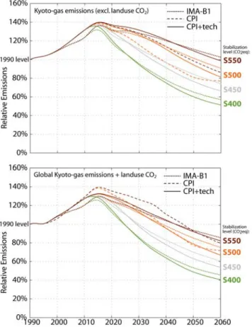
The emissions of the emission pathways for stabilization at 550, 450 and 400ppm CO2eq concentrations for the three scenarios can be summarized by their GWP-weighted sum for illustrative purposes, as illustrated in Figure 5. Clearly, there are different pathways that can lead to the ultimate stabilisation level. Here, for all default pathways we assume that the emission reductions take place early in the scenario period and the global emissions peak around 2015, in order to avoid pathways that exceed an annual reduction of 2% per year (at least not over longer time periods). The reason is that a faster reduction might be difficult to achieve given the inertia in the energy system: electric power plants, for instance, have a technical lifetime of 30 years or more. Fast
reduction rates would require early replacement of existing plants, which is expensive.
For all stabilisation scenarios, the global reduction rates remain below 2%/year for the whole scenario period, except for the pathways at 400ppm CO2eq with maximum reduction rates of 2.5-3%/yr over 20 years.
Figure 5 - Global emissions excluding and including LUCF CO2 emissions for the
stabilization scenarios at 550, 500, 450 and 400 ppm CO2 equivalent concentrations for the
three scenarios (CPI, CPI tech and IMA-B1)10.
If we delay the peaking of the global emissions until 2020, this needs to be compensated by steeper reductions hereafter. Now only for the 550ppm CO2eq for the B1 and CPI tech scenario there will be pathways, which do not exceed the 2%/yr limit. For 400 and 450ppm CO2eq, all three baseline scenarios lead to maximum yearly reduction rates above 3.5 and 2.5 %, respectively, for at least 20 years if emission reductions were delayed. For 500ppm CO2eq, this rate reaches 2.5% for 15 years under the delayed scenario.
Under the three default scenario for stabilization at 550ppm CO2eq, Kyoto-gas emissions (including LUCF CO2) would approximately have to return to their 1990 levels by 2050. We also see that higher near-term emissions need to be compensated by lower future emissions (compare CPI and CPI-tech
10 For the CPI scenario the current assumptions about abatement
potential and costs result in no emission pathways for 450 and 400 ppm CO2 equivalent concentrations.
with B1). For stabilization at 500ppm CO2eq, global Kyoto-gas emissions would need 10 to 20% below 1990 levels in 2050. The reduction requirements become as high as 50-60% and 30-40% below 1990 levels in 2050 to reach the 400ppm and 450ppm CO2eq target, respectively (see Figure 5). In general, when we compare the reductions for the different concentration levels, we find about 15-20% additional reductions by 2050 are needed for every 50ppm lower stabilisation level.
Analysing the emission reductions of the Kyoto gases without LUCF CO2 emissions, but still assuming that the LUCF CO2 emissions decrease as specified, we see that the global Kyoto gas emission reductions are less: 35-45% and 15-25% below 1990 levels by 2050 to reach 400ppm and 450ppm CO2eq target.
Figure 6 shows the global fossil CO2 emissions. The reductions for the fossil CO2 emissions are in general somewhat higher than the reductions of all Kyoto gas emissions for the lower concentration targets (400 and 450ppm CO2eq), as we assume less abatement potential for the non-CO2 gases in particular from agricultural and land-use related sources. The reduction requirements for the fossil CO2 emissions are the highest for the CPI scenario, as this scenario assumes higher LUCF CO2 emissions than the other two scenarios (B1, CPI-tech).
Figure 6 - Global fossil CO2 emissions,
otherwise as figure 5. In addition, global fossil CO2 emissions of the six illustrative
non-mitigation IPCC SRES scenarios [46] are shown.
4. Global emission abatement costs
In its Third Assessment Report (TAR) [47] the IPCC presents estimates for macro-economic costs of stabilisation of the CO2 concentration and these estimates also cover a considerable range. For stabilisation of the CO2 concentration at 450ppm (comparable to 500-525ppm CO2eq.), GDPreductions for 2050 are in the order of 2.5-3.0% (the range associated with scenario A1b and B2).
These GDP costs have to be seen in perspective, though. On the one hand, such long-term GDP abatement costs are approximately equivalent to a delay of only a couple of years in regard to the point in time, when the World might experience a twenty fold increase in its GDP around 2100 compared to present levels [48, 49]. On the other hand, avoided climate damages and ancillary benefits are not included in such cost estimates, although they might be comparable in scale. Here, we present some preliminary results11 of the global abatement costs12 as percentage of world GDP for the different CO2 equivalent concentration levels (Figure 7). We see that the global costs increase as a result of increasingly tight concentration levels. All emission pathways show a rapidly increase of the costs till 2050, and then a decrease for most of the scenarios, except for pathway leading to 500ppm CO2 eq. under the CPI baseline. 0.0 0.5 1.0 1.5 2.0 2000 2025 2050 2075 2100 550 0.0 0.5 1.0 1.5 2.0 2000 2025 2050 2075 2100 500 0.0 0.5 1.0 1.5 2.0 2000 2025 2050 2075 2100 CPI CPI t ech B1 450 0.0 0.5 1.0 1.5 2.0 2000 2025 2050 2075 2100 400
Figure 7 - Global abatement costs as % of GDP for the stabilization scenarios at (a) 550ppm, (b) 500ppm, (c) 450ppm and (d) 400ppm CO2
equivalent concentrations for the three scenarios (CPI, CPI tech and IMA-B1).
The Figure also shows that the global abatement costs are even more influenced by the baseline emissions and the assumed technical change improvements of the abatement potentials
11 The costs figures presented here should be seen as provisional,
and may change due to ongoing research related to the abatement potential and reduction costs for all greenhouse gases.
12 The costs calculated only represent the direct-cost effects based
on MAC curves but not the various linkages and rebound effects via the economy or impacts of carbon leakage; i.e. there is no direct link with macro-economic indicators such as GDP losses or other measures of income of utility loss.
and costs, than the final concentration stabilisation level. More specifically, the baseline emissions directly determine the reductions that are required to reach the emission profile for stabilisation. In addition, the baseline assumptions also indirectly influence the abatement potential, in particular, assumptions related to costs of different technologies. Finally, the economic assumptions obviously influence the relative cost measures such as GDP losses or abatement costs as percentage of GDP. Another crucial uncertainty is the rate at which the potential and abatement costs for CO2 and non-CO2 emission reductions develops in time (compare the CPI and CPI tech baseline scenario – see section 2).
5. Conclusions
This study uses a method to derive multi-gas emission pathways by a method that calculates the cost-optimal mixes of greenhouse gases reductions for a given global emissions pathway. The study presents emission pathways for different CO2 equivalent concentration stabilisation levels, i.e. 550, 500, 450 and 400 ppm CO2 equivalent.
This analysis shows that an emission pathway leading to a 550ppm CO2 equivalent stabilisation is unlikely to meet the climate target of limiting global mean temperature rise to 2°C above pre-industrial levels (EU 2oC target). In order to achieve this EU target with levels of certainty of more than 50%, greenhouse gas concentrations need to be stabilised below 450 CO2 equivalent or lower, requiring global emissions to peak within the next two decades, followed by substantial overall reductions by as much as 30 to 60% (incl. LUCF CO2 emissions) in 2050 compared to 1990 levels (450/400ppm CO2eq). Further delay in peaking leads to delayed, but much steeper reductions.
The analysis shows that the global reductions, and thus the abatement costs, much depends on the emission growth in the baseline scenario, as well as further developments of the abatement potential and reduction costs for all greenhouse gases in the future due to technology progress and removal of implementation barriers. These two factors also highly influence the certainty of meeting more stringent climate targets. Lower baseline emissions also lead to a later peaking of the global emissions, and therefore more allowable emissions after peaking. However, the allowable delay in the peaking emissions is limited, less than 5-10 years delay, and in order to achieve the lower stabilisation levels it is still needed to stabilise the global emissions within the next two decades.
6. Acknowledgements
The authors thank Marcel Berk, Bas Eickhout, Paul Lucas and Detlef van Vuuren (RIVM, the
a
b
c
Netherlands) for comments and suggestions in various stages of the research.
7. References
[1] European-Council: 1996, 'Communication on Community Strategy on Climate Change, Council Conclusions', European Commission, Brussels. [2] Smith, J.B., Schellnhuber, H.-J. and Mirza, M.Q.M.:
2001, 'Vulnearability to Climate Change and Reasons for Concern: A Synthesis', in McCarthy, J.J., Canziani, O.F., Leary, N.A., Dokken, D.J. and White, K.S. (eds.), Climate Change 2001: Impacts, Adaptation, and Vulnerability, Cambridge University Press, Cambridge, UK, pp. 1042.
[3] Hare, W.: 2003, 'Assessment of Knowledge on Impacts of Climate Change – Contribution to the Specification of Art. 2 of the UNFCCC'. Potsdam, Berlin, WBGU - German Advisory Council on Global Change.
http://www.wbgu.de/wbgu_sn2003_ex01.pdf
[4] ACIA: 2004, Impacts of a Warming Arctic - Arctic Climate Impact Assessment, Cambridge University Press, Cambridge, UK.
[5] Allen, M.R. and Lord, R.: 2004, 'The blame game - who will pay for the damaging consequences of climate change?' Nature 432, 2 December 2004. [6] Stott, P.A., Stone, D.A. and Allen, M.R.: 2004,
'Human contribution to the European heatwave of 2003', Nature 432, 610-614.
[7] Hare, B. and Meinshausen, M.: 2004, 'How much warming are we committed to and how much can be avoided?' PIK Report. Potsdam, Potsdam Institute for Climate Impact Research: 49. No. 93
http://www.pik-potsdam.de/publications/pik_reports [8] Meinshausen, M.: 2004, 'On the Risk to Overshoot
2°C - submitted manuscript', Avoiding Dangerous Climate Change, tba, Hadley Centre Exeter, UK, pp.
[9] Reilly, J., Prinn, R.G., Harnisch, J., Fitzmaurice, J., Jacoby, H.D., Kicklighter, D., Stone, P.H., Sokolov, A.P. and Wang, C.: 1999, 'Multi-gas Assessment of the Kyoto Protocol', Nature 401, 549-555.
[10] Hayhoe, K., Jain, A., Pitcher, H., MacCracken, C., Gibbs, M., Wuebbles, D., Harvey, R. and Kruger, D.: 1999, 'Costs of multigreenhouse gas reduction targets for the USA', Science 286, 905-906. [11] Tol, R.: 1999, 'The marginal Cost of greenhouse gas
emissions', Energy Journal 20, 61-81.
[12] Manne, A.S. and Richels, R.G.: 2001, 'An alternative approach to establishing trade-offs among
greenhouse gases', Nature 410, 675-677. [13] van Vuuren, D.P., den Elzen, M.G.J., Berk, M.M.,
Lucas, P., Eickhout, B., Eerens, H. and Oostenrijk, R.: 2003, 'Regional costs and benefits of alternative post-Kyoto climate regimes'. Bilthoven, the
Netherlands, National Institute for Public Health and the Environment. RIVM-report 728001025 [14] den Elzen, M.G.J., Lucas, P. and van Vuuren, D.:
2004, 'Abatement costs of post-Kyoto climate regimes', Energy Policy (in press).
[15] Hansen, J., Sato, M., Ruedy, R., Lacis, A. and Oinas, V.: 2000, 'Global warming in the twenty-first century: An alternative scenario', Proceedings of the National Academy of Sciences of the United States of America 97, 9875-9880.
[16] Meinshausen, M., Hare, B., Wigley, T.M.L., van Vuuren, D., den Elzen, M.G.J. and Swart, R.: submitted, 'Multi-gas emission pathways to meet arbitrary climate targets', Climatic Change, 50. [17] Wigley, T.M.L., Richels, R. and Edmonds, J.A.:
submitted, 'Overshoot Pathways to CO2
stabilization in a multi-gas context', in Schlesinger, M.E. and Weyant, J.P. (eds.), Human Induced Climate Change: An Interdisciplinary Perspective, Cambridge University Press, Cambridge, UK. [18] Richels, R., Manne, A. and Wigley, T.M.L.: 2004,
'Moving beyond concentrations: the challenge of limiting temperature change', AEI-Brookings Joint Center for Regulatory Studies. Working-Paper 04-11
[19] Fuglestvedt, J.S., Berntsen, T.K., Godal, O., Sausen, R., Shine, K.O. and Skodvin, T.: 2003, 'Assessing metrics of climate change - current methods and future possibilities', Climatic change 58, 267-331. [20] O'Neill, B.C.: 2003, 'Economics, natural science and
the costs of global warming potentials', Climatic change 58, 251-260.
[21] Cubasch, U., Meehl, G.A., Boer, G.J., Stouffer, R.J., Dix, M., Noda, A., Senior, C.A., Raper, S. and Yap, K.S.: 2001, 'Projections of Future Climate Change', in Houghton, J.T., Ding, Y., Griggs, D.J., Noguer, M., van der Linden, P.J., Dai, X., Maskell, K. and Johnson, C.A. (eds.), Climate Change 2001: The Scientific Basis, Cambridge University Press, Cambridge, UK.
[22] Raper, S.C.B. and Cubasch, U.: 1996, 'Emulation of the results from a coupled general circulation model using a simple climate model', Geophysical
Research Letters 23, 1107-1110.
[23] Eickhout, B., den Elzen, M.G.J. and van Vuuren, D.P.: 2003, 'Multi-gas emission profiles for stabilising greenhouse gas concentrations'.
Bilthoven, the Netherlands. RIVM-report 728001026 [24] Morita, T., Nakicenovic, N. and Robinson, J.: 2000,
'Overview of mitigation scenarios for global climate stabilization based on new IPCC emission
scenarios (SRES)', Environmental Economics and Policy Studies 3, 65-88.
[25] Swart, R., Mitchell, J., Morita, T. and Raper, S.: 2002, 'Stabilisation scenarios for climate impact assessment', Global Environmental Change 12, 155-165.
[26] Meinshausen, M., Hare, B., Wigley, T.M.L., van Vuuren, D.P., den Elzen, M.G.J. and Swart, R.: 2004, 'Mulit-gas emission pathways to meet climate targets', Climatic change (submitted).
[27] den Elzen, M.G.J. and Lucas, P.: 2003, 'FAIR 2.0: a decision-support model to assess the environmental and economic consequences of future climate regimes, www.rivm.nl/fair'. Bilthoven, the Netherlands. RIVM-report 550015001
[28] den Elzen, M.G.J.: 2002, 'Exploring climate regimes for differentiation of future commitments to stabilise greenhouse gas concentrations', Integrated Assessment 3, 343-359.
[29] IMAGE-team: 2001, 'The IMAGE 2.2 implementation of the SRES scenarios. A comprehensive analysis of emissions, climate change and impacts in the 21st century'. Bilthoven, the Netherlands. CD-ROM publication 481508018
[30] de Vries, H.J.M., D.P. van Vuuren, Elzen, M.G.J.d. and Janssen, M.A.: 2002, 'The Targets Image
Energy model regional (TIMER) - Technical documentation'. Bilthoven, the Netherlands, National Institute of Public Health and the Environment (RIVM). RIVM report 461502024 [31] Wigley, T.M.L. and Raper, S.C.B.: 2001,
'Interpretation of high projections for global-mean warming', Science 293, 451-454.
[32] Wigley, T.M.L. and Raper, S.C.B.: 2002, 'Reasons for larger warming projections in the IPCC Third Assessment Report', journal of climate 15, 2945-2952.
[33] Wigley, T.M.L.: 2003, 'MAGICC/SCENGEN 4.1: Technical Manual'. Boulder, CO, UCAR - Climate and Global Dynamics Division.
http://www.cgd.ucar.edu/cas/wigley/magicc/index.ht ml
[34] IPCC: 2001, Climate Change 2001: Mitigation, Cambridge University Press, Cambridge, UK. [35] van Vuuren, D.P., de Vries, H.J.M., Eickhout, B. and
Kram, T.: 2004, 'Responses to Technology and Taxes in a Simulated World', Energy Economics
26.
[36] van Vuuren, D.P., Eickhout, B., Lucas, P.L. and den Elzen, M.G.J.: 2004, 'Long-term multi-gas
scenarios to stabilise radiative forcing - exploring costs and benefits within an integrated assessment framework', Energy Policy (accepted).
[37] DeAngelo, B.J., DelaChesnaye, F.C., Beach, R.H., Sommer, A. and Murray, B.C.: 2004, 'Methane and nitrous oxide mitigation in agriculture', Energy Policy (in press).
[38] Delhotal, K.C., DelaChesnaye, F.C., Gardiner, A., Bates, J. and Sankovski, A.: 2004, 'Mitigation of methan and nitrous oxide emissions from waste, energy and industry', Energy Policy (in press). [39] Schaefer, D.O., Godwin, D. and Harnisch, J.: 2004,
'Estimating future emissions and potential
reductions of HFCs, PFCs and SF6', Energy Policy
(in press).
[40] Graus, W., Harmelink , M. and Hendriks, C.: 2004, 'Marginal GHG-Abatement curves for agriculture'. Utrecht, the Netherlands, Ecofys.
[41] Nakicenovic, N. and Riahi, K.: 2003, 'Model runs with MESSAGE in the Context of the Further Development of the Kyoto-Protocol'. Berlin, WBGU - German Advisory Council on Global Change: 54. [42] Azar, C., Linddgren, K., Larson, E. and Möllersten,
K.: 2004, 'Carbon capture and storage from fossil fuels and biomass - Costs and potential role in stabilizing the atmosphere', Climatic change (submitted).
[43] Hansen, J., Russell, G., Lacis, A., Fung, I., Rind, D. and Stone, P.: 1985, 'Climate Response-Times - Dependence on Climate Sensitivity and Ocean Mixing', Science 229, 857-859.
[44] Raper, S.C.B., Gregory, J.M. and Stouffer, R.J.: 2002, 'The Role of Climate Senstivity and Ocean Heat Uptake on AOGCM Transient Temperature Response', Journal of Climate 15, 124-130. [45] Folland, C.K., Rayner, N.A., Brown, S.J., Smith,
T.M., Shen, S.S.P., Parker, D.E., Macadam, I., Jones, P.D., Jones, R.N., Nicholls, N. and Sexton, D.M.H.: 2001, 'Global temperature change and its uncertainties since 1861', Geophysical Research Letters 28, 2621-2624.
[46] Nakicenovic, N., Alcamo, J., Davis, G., de Vries, B., Fenhann, J., Gaffin, S., Gregory, K., Grübler, A.,
Jung, T.Y., Kram, T., Emilio la Rovere, E., Michaelis, L., Mori, S., Morita, T., Pepper, W., Pitcher, H., Price, L., Riahi, K., Roehrl, A., Rogner, H., Sankovski, A., Schlesinger, M., Shukla, P., Smith, S., Swart, R., van Rooyen, S., Victor, N. and Dadi, Z.: 2000, Special Report on emissions scenarios, Cambridge University Press, Cambridge, UK.
[47] IPCC: 2001, Climate Change 2001.Synthesis Report, Cambridge University Press, Cambridge, UK. [48] Azar, C. and Schneider, S.H.: 2002, 'Are the
economic costs of stabilising the atmosphere prohibitive?' Ecological Economics 42, 73-80. [49] Azar, C. and Schneider, S.H.: 2003, 'Are the
economic costs of (non-)stabilizing the atmosphere prohibitive? A response to Gerlagh and Papyrakis', Ecological Economics 46, 329-332.