Correcting air pollution time series for meteorological variability. With an application to regional PM10 concentrations

(1)

With an application to regional PM10 concentrations

H. Visser and H. Noordijk

This investigation has been performed by order and for the account of RIVM, within the framework of project S/722601, Measuring and Modelling.

(2)

(3)

Abstract

It is well-known that a large part of the year-to–year variation in annual distribution of daily concentrations of air pollutants is due to fluctuations in the frequency and severity of meteorological conditions. This variability makes it difficult to estimate the effectiveness of emission control strategies.

In this report we have demonstrated how a series of binary decision rules, known as Classification And Regression Trees (CART), can be used to calculate pollution concentrations that are standardized to levels expected to occur under a fixed (reference) set of meteorological conditions. Such meteo-corrected concentration measures can then be used to identify ‘underlying’ air quality trends resulting from changes in emissions that may otherwise be difficult to distinguish due to the interfering effects of unusual weather patterns. The examples here concern air pollution data (daily concentrations of SO2 and PM10).

However, the methodology could very well be applied to water and soil applications. Classification trees, where the response variable is categorical, have important applications in the field of public health. Furthermore, Regression Trees, which have a continuous response variable, are very well suited for situations where physically oriented models explain (part of) the variability in the response variable. Here, CART analysis and physically oriented models are not exclusive but complementary tools.

(4)

Samenvatting

Dag-op-dag-variaties in meteorologische condities zijn een belangrijke oorzaak van variaties in het concentratieverloop van luchtveronreinigende stoffen. Deze aan meteorologie gekoppelde variaties werken ook door in jaargemiddelde concentraties. Daarom is het moeilijk om te beoordelen in hoeverre jaargemiddelde patronen van luchtverontreinigende componenten beïnvloed worden door emissiereducties. Zo’n beoordeling is zeer beleids-relevant omdat emissiereducties over het algemeen gepaard gaan met hoge kosten. Daarom zal er, om een een maatschapppelijke draagvlak te garanderen, een relatie gelegd moeten worden tussen trends in antropogene emissies enerzijds en trends in concentraties anderzijds. In dit rapport tonen we aan hoe met behulp van een reeks binaire beslisregels, bekend staand onder de naam Classificatie- en Regressiebomen (Eng: CART), gemeten concentraties getransformeerd kunnen worden naar concentraties die er zouden zijn geweest onder standaard meteorologische condities. Deze meteo-gecorrigeerde concentraties kunnen vervolgens gebruikt worden om trends in luchtkwaliteit beter te identificeren.

CART-analyse en meer specifiek Regressieboom-analyse, heeft een aantal voordelen boven andere statistische technieken. In de eerste plaats is de methode parametervrij. Dat wil zeggen dat er geen aannames hoeven te worden gedaan over onderliggende kansverdelingen. In de tweede plaats mogen de relaties tussen een responsvariabele (concentratie van stof X) en de predictors (variabelen zoals temperatuur, neerslag, windrichting of windsnelheid) in hoge mate niet-lineair zijn. In de derde plaats zijn resultaten van een CART-analyse relatief eenvoudig te interpreteren.

Hoewel de voorbeelden in dit rapport gericht zijn op luchtverontreiniging, is de methode zeer geschikt voor andere milieuvelden zoals water- en bodemverontreiniging. Regressiebomen, waar de responsvariabele continu is, zijn van ook van belang voor situaties waar fysisch-georiënteerde modellen een deel van de variabiliteit van de responsvariabele beschrijven. Regressieboom-analyse is complementair aan deze fysische modellen. Classificatiebomen, waar de responsevariabele nominaal is, hebben grote relevantie voor het onderzoeksgebied van de Volksgezondheid.

We hebben verfijningen ontwikkeld voor de Regressieboom-benadering zoals beschreven door Dekkers en Noordijk (1997). Deze verfijningen omvatten: (i) controle van de data op uitbijters, ontbrekende waarnemingen en hoge correlaties tussen de predictors, (ii) controle op de responsvariabele of transformaties nodig zijn, (iii) cross-validatie van de geschatte Regressieboom, en (iv) evaluatie van de voorspelkracht van een Regressieboom in vergelijking met alternatieve voorspelmethoden.

Als een case study hebben we de methodologie toegepast op metingen van fijnstof (PM10).

We hebben 9 regionale stations geanalyseerd met metingen over de periode 1992-2001. De resultaten laten zien dat:

• regressieboom-modellen die gebaseerd zijn op maandgemiddelde concentraties, beter voldoen dan modellen op daggemiddelde waarden;

• langjarige trends in concentraties niet beïnvloed worden door variaties in meteorologie; • concentraties een dalende tendens vertonen, net als emissies. Na correctie voor

natuurlijke emissiebronnen (zeezout, opwaaiend stof en de achtergrondconcentratie van het Noordelijk halfrond) blijken emissies sterker te dalen dan concentraties.

(7)

Summary

It is well-known that part of the year-to–year variation in annual distribution of daily concentrations of air pollution in ambient air is due to fluctuations in the frequency and severity of meteorological conditions. This variability makes it difficult to estimate the effectiveness of emission control strategies.

In this report we have demonstrated how a series of binary decision rules, known as Classification And Regression Trees (CART), can be used to calculate pollution concentrations that are standardized to levels that would be expected to occur under a fixed (reference) set of meteorological conditions. Such adjusted concentration measures can then be used to identify ‘underlying’ air quality trends resulting from changes in emissions that may otherwise be difficult to distinguish due to the interfering effects of unusual weather patterns.

CART analysis, and more specifically Regression Tree analysis, has a number of advantages over other classification methods, such as Multiple Regression. First, it is inherently non-parametric. In other words, no assumptions have to be made a priori regarding the underlying distribution of values of the response variable or predictor variables. Second, the relationship between the response variable (concentration of a pollutant) and predictors (meteorological variables) may be highly non-linear. Third, the estimation results of a CART analysis are relatively easy to interpret.

Although the examples given here concern air pollution, the methodology could very well be used for water and soil applications. Regression Trees, having a continuous response variable, are very well suited to situations where physically oriented models explain (part of) the variability of the response variable. Here, Regression Trees and physically oriented models are not exclusive but complementary tools. Furthermore, Classification Trees, where the response variable is categorical, have important applications in the field of Public Health. We have refined the methodology of Dekkers and Noordijk (1997) for Regression Trees. Refinements comprise (i) checks on the data for outliers, missing values and multi-collinearity among the predictors, (ii) checks for transformation of concentrations prior to the estimation of a Regression Tree, (iii) cross-validation of the final optimal tree and (iv) evaluation of the predictive power of the final tree in relation to alternative (rival) models. The Regression Tree methodology, applied as a case study to nine regional stations of PM10

in the Netherlands, has yielded the following results:

• RT models based on monthly concentrations outperformed those based on daily data. Apparently, monthly averaged meteorology is more influenced by large-scale meteorology in Europe, governing periods with extreme concentrations;

• Long-term trends in PM10 concentrations have not been not influenced by meteorological

variability.

• Regional concentration trends show large similarities to trends in emissions. If we correct concentrations for natural emission sources (sea salt, wind-blown dust and northern hemisphere background concentrations), emissions decrease faster than concentrations.

(8)

(9)

1. Introduction

1.1 Why statistical modelling?

A wide diversity of mathematical models is applied within the RIVM Office for Environmental Assessment (MNP in Dutch). These models are based on physical, chemical, meteorological and biological relationships. Reality is approximated as well as possible in these models. What ‘as well as possible’ means, can be verified by environmental measurements.

We will denote the model-based approach here as ‘white box modelling’. In many cases

white box modelling will give a deterministic approach to reality. As an example we can cite

the OPS model (Jaarsveld, 1995) by which the dispersion and deposition of a number of air pollution components are modelled as a function of emissions and meteorology.

Contrary to white box modelling we also have so-called ‘black box modelling’. With this second approach we mean the modelling of measurements on the basis of statistical principles. A measurement series is seen as a deterministic signal and a stochastic residual signal, the ‘noise’. A series of measurements can therefore be viewed as a possible

realization of reality. Some slightly different outcomes would have been equally likely. We

will denote these series as ‘time series’.

Within the statistical approach, relationships (or associations) are estimated by calculating correlation. Correlation points to the similarity in patterns, but does not prove causality. Therefore, we use the term ‘black box’. Examples of black box modelling are illustrated in Multiple Regression models, ARIMA models or methods based on the Regression Tree, described in this report.

The mixture of white box and black box modelling is called grey box modelling. If a physical model only partly describes reality, we can describe the ‘difference’ between white box model

predictions and reality (the measurements) by statistical modelling.

An example of grey box modelling is the modelling of PM10-concentrations in the

Netherlands by the OPS-model. The OPS-model describes the anthropogenic contribution to measured PM10 concentrations. However, by doing so, only half the concentration variations

are explained. Research has shown that the ‘rest’ is largely explained by the share of natural sources (Visser et al., 2001). From this moment, we could describe and predict the difference between measurements and OPS-predictions statistically, using such geostatistical techniques as Universal Kriging.

In the absence of a physical model, it is clear that statistical models can play an important role in finding relevant relations. But even with a physical description of our environmental reality, statistical modelling can be of importance. Statistical inferences are pre-eminently suited as a diagnostic tool for unraveling and explaining differences between measurements and the predictions of physically oriented models. Three examples follow:

(10)

1) The correction of environmental measurements for meteorological conditions. Dekkers and Noordijk (1997) describe a generic method based on Regression Trees by which the time series of air pollution components (PM10, SO2, NOx, O3, and black

smoke) is corrected for meteorological conditions. Such a correction is of great importance for policy-makers because after correction one can make inferences on the influence of emission reductions on the actual ambient concentrations with much more certainty.

Statistical techniques such as Regression Tree analysis or Multiple Regression yield insights, which may be defined later in terms of physical relationships. An example is given in Chapter 5 for the time series of PM10 concentrations. It appears that months with extreme droughts

and cold periods correspond to months with very high PM10 concentrations. This sort of

relationship has not been taken into account in RIVM models such as OPS or EUROS, but could be formulated into a physical framework and added to these models.

2) A second example is found in the field of forecasting. For components such as PM10

and O3 RIVM produces smog forecasts on television (Teletekst) 1 and 2 days in

advance. Simple statistical models, such as the autoregressive model with two parameters, have often been found to outperform forecasts of complex white models. Here, forecasts of black and white models could be evaluated on a test set, where the best method is declared the winner. Or one might choose to combine forecasts of both models (Makridakis et al., 1982).

3) A third example of great importance to the MNP, is the sensitivity analysis of complex computational-intensive models (Saltelli et al., 2000). One method in this field is to find the sensitivity of a certain output variable, y, to variations in the input variables, x = (x1, x2, …, to xm). Which xi has the largest impact and which the

lowest? If the computational time of one model run is in the order of hours or even days, this question is not trivial. Now, if we calculate y for a limited number of input combinations x, we can estimate a Regression Tree model or a Multiple Regression model between these sets (y,x). Once having estimated a black box model, one can easily deduce an ordering in importance of the various input variables.

Such an exercise has been performed for the RIVM model PcDitch, consisting of 100 response variables and a set of 200 predictors. Screening the 200 predictors by Regression Tree analysis yielded a set of 20 predictors governing specific response variables.

(11)

Physically oriented models and statistical models such as Regression Trees, are not rivals but complementary tools in explaining what we know and what we don’t know about our data (Photo: H. Visser).

(12)

1.2 The need for meteo corrections

The analysis of a series of measurements is generally done to show trends in concentrations that are influenced by human activities. The point is to clarify how society influences the ambient air pollution concentrations. On the one hand, the ongoing economic growth leads to more production and emissions, while, on the other, environmental abatement policies and the abatement of emissions leads to mitigation of concentrations. A long-term time series of measurements may give us insight into the influence of the economy and environmental policy.

A third influence on the ambient concentrations is that of the meteorology. The influence of the weather is not constant in time. For example, taking particulate matter (PM) and SO2, we

know that a cold winter in the Netherlands will yield higher average concentrations. These higher PM concentrations are partly the result of more transport from abroad, as sub-zero temperatures are usually accompanied by a continental air flow that is generally more polluted than air masses from the Atlantic Ocean. During a period of frost the general dispersion conditions are such that inversions occur more often. Furthermore, emissions tend to be higher during these periods as heating of homes consumes more energy and cold starts of cars produce more pollution. During a long cold spell high wind speeds may also re-suspend airborne crustal material from the barren anddry fields. A year with more rain than usual will lead to lower concentrations of PM, mainly because of either rainout or washout, and to a lesser extent because it is harder for crustal material to become re-suspended when soils are moist.

In this report we will demonstrate how a series of binary decision rules, known as Classification And Regresion Trees (CART), can be used to calculate pollution concentrations that are standardized to levels that would be expected to occur under a fixed (reference) set of meteorological conditions. Such meteo-corrected concentration measures can then be used to identify ‘underlying’ air quality trends resulting from changes in emissions that may otherwise be difficult to distinguish due to the interfering effects of unusual weather patterns.

1.3 Regression Tree analysis

A method has been developed at the RIVM to analyse the influence of meteorology on the trends in air pollution (Dekkers and Noordijk, 1997). This method uses the ambient air pollution concentrations in the Netherlands in combination with daily-averaged meteorological values. The meteorological factors influencing concentrations are divided into different classes by way of Regression Trees (Breiman et al., 1984). Regression Trees comprise part of the so-called Classification and Regression Trees (CART) methodology. The difference between Classification Trees and Regression Trees is that the response variable is categorical in Classification Trees and continuous in Regression Trees.

Regression Tree analysis (RTA) is a statistical technique that divides the set of measurements into two sub-sets on the basis of meteorological criteria. The criterion for the division of the sub-sets is the minimization of the variance of the two sub-sets. After this first step in the analysis, one of the sub-sets is itself again divided into two new sub-sets, with again the

(13)

the influence of meteorology on the concentrations.

Once we have generated a tree, we want to check if all the nodes in the tree are needed or if we should prune the tree. The rationale for pruning the tree is that we want to have a model for our data that is as parsimonious as possible, while keeping certain desirable characteristics in tact (such as the predictive power of the tree, see below).

The final nodes of the tree are called ‘leaves’. By averaging all concentrations on days that correspond to that specific leaf we get an RT prediction for days that fall in the particular meteo class. It should be noted that the term ‘predictions’ is used in the common statistical sense, i.e. we may predict both values within the time series available and predict the future (forecasting).

The ‘predictive power’ of the tree is found by calculating the mean squared error of the prediction errors. The prediction error stands for the difference between the actual concentration on a specific day and the corresponding leaf prediction (the average value of all concentrations of falling in that leaf).

Once a suitable tree has been estimated, we want to correct annual averaged concentrations or annual percentiles for meteorological conditions. Basically, there are two approaches. The first approach has been proposed by Stoeckenius (1991). For every year the frequency of occurrence of a meteo class is determined, the frequency of occurrence determines the actual value of the correction factor. As an example, when the meteo class of tropical days normally occurs three times a year and in a specific year there are six of these days, the calculation of these tropical days in the yearly average is less than average and the correction factor becomes 0.5. However, when by chance a certain meteo class does not occur, an estimate is made of the expected concentrationsby using concentrations from other years in that specific meteo class. We will describe an expanded version of this procedure in more detail in Noordijk and Visser (in prep.).

A second approach is to estimate the mean concentration µy for all concentrations yt . If we

denote the predicted concentration at time t as ŷt, then we define the particular concentrations

due to meteorological conditions as the difference between ŷt and µy. Finally, the

meteo-corrected concentration on day t is ycorr,t= yt – (ŷt – µy) . Now, annual averaged

concentrations or percentiles are simply calculated on the corrected daily data ycorr,t. In this

document we will apply this correction approach, while in Noordijk and Visser (in prep.) we will evaluate both meteo-correction methods.

CART analysis, and more specifically Regression Tree analysis, has been applied in many fields. For references see Ripley (1996) and Venables and Ripley (1997). Many references can by found via search path CART ‘Regression Tree*’. However, Regression Tree analysis has not been applied as frequently in air pollution research. Two references on application to ozone data are Stoeckenius (1991) and Gardner and Dorling (2000). In the latter article Regression Tree analysis, Linear Regression and Multilayer Perceptron Neural Networks are compared using hourly surface ozone concentrations.

(14)

1.4 Refinements

We apply Regression Tree analysis to time series of air pollutants. By doing so, we have to ensure that our final tree model:

• fits the data well; • is physically plausible;

• is able to withstand a comparison to alternative (rival) models.

Harvey (1989, pages 13-14) summarizes the criteria for a good model as proposed in the econometric literature. These criteria equally hold for environmental time-series models and, more specifically, for Regression Tree models.

The following six criteria from Harvey (1989) represent an elaboration of the three points above:

(a) Parsimony. A parsimonious model is one that contains a relatively small number of parameters. Other things being equal, a simpler model is preferred to a complicated one. In general, there can be considerable advantages in starting with a general model and then simplifying it on the basis of statistical tests.

(b) Data coherence. Diagnostic checks are performed to see if the model is consistent with the data. The essential point is that the model should provide a good fit to the data and the residual, be relatively small, and approximately random.

(c) Consistency with prior knowledge. The size and magnitude of parameters in the model should be consistent with prior information. And the same should hold for the classification rules from a specific Regression Tree. This information should relate to a physical, chemical or meteorological context.

(d) Data admissibility. A model should be unable to predict values which violate definitional constraints. For example, concentrations cannot be negative.

(e) Validation (structural stability). The model should provide a good fit, inside and outside the sample. In order for this to be possible, the parameters or classification rules should be constant within the sample period and this constancy should carry over to data not in the sample period. The latter data could fall within the timespan of the sample (principle of cross validation) or could lie in the future, the post-sample period.

(f) Encompassing. A model is said to encompass a rival formulation if it can explain the results given by the rival formulation. If this is the case, the rival model contains no information that might be of use in improving the preferred model. In order fulfil its encompassing role, a model does not need to be more general than its rivals.

To meet these criteria as best as possible, we have made a number of refinements to the approach given by Dekkers and Noordijk (1997). These refinements comprise diagnostic checks to the data set prior to the estimation of a specific Regression Tree, transformation of data, analysis of residuals, testing the stability of the final tree by the principle of cross-validation, and comparison of Regression-Tree performance to alternative/rival models. We will describe these refinements in detail in §2.4.

(15)

In Chapter 2 we will describe the Regression Tree approach in more detail, illustrating the theoretical considerations with an example on SO2 concentrations. Chapter 3 will be devoted

to a short, in-depth, description on the implementation of a Regression Tree analysis in S-PLUS. S-PLUS is the standard statistical software package of RIVM (Dekkers, 2001). More details on this topic will be given in Visser (in prep.). Our approach has resulted in an eight-step procedure, summarized in §2.9. In Chapter 4 we will illustrate this eight-eight-step procedure by use of a simulation example. Simulated examples have the advantage that the correct solutions are known a-priori and that the estimation procedure can be judged on its merits. In Chapters 5 and 6 we will give case studies using the methodology given in Chapter 2. Chapter 5 deals with nine regional PM10 stations in the Netherlands. In Chapter 6 we will

analyse 22 regional SO2 stations. For both pollutants we will show that meteo-corrected

regional concentrations show the same long-term trend as the uncorrected data. The extreme concentrations in 1996, and to a lesser extent 1997, appear to originate from unusual cold and dry winters at that time.

(16)

(17)

2. Regression Tree analysis

2.1 Method

Tree-based modelling is an exploratory technique for uncovering structure in data and is increasingly used for:

• devising prediction rules that can be rapidly and repeatedly evaluated; • screening variables;

• assessing the adequacy of linear models; • summarizing large multivariate data sets.

Tree-based models are useful for solving both classification and regression problems. In these problems, there is a set of classification or predictor variables, x = (x1, x2, … , xm), and

a single-response variable, y. In the literature tree-based models are denoted by the abbreviation CART (Classification And Regression Trees).

If y has discrete values, classification rules take the form: If x1 < 2.3 and x3∈ {A,B}

then y is most likely to be in level 5

If y is numeric, regression rules for description or prediction take the form: If x2 < 2.3 and x9∈ {C,D,F} and x5≥ 3.5

then the predicted value of y is 4.75

In the first case we speak of a classification tree, and in the second, of a regression tree. A classification or regression tree is the collection of many such rules displayed in the form of a binary tree, hence the name. The rules are determined by a procedure known as recursive

partitioning.

Tree-based models provide an alternative to linear and additive models for regression problems, and to linear and additive logistic models for classification problems.

Compared to linear and additive models, tree-based models have the following advantages: • easier interpretation of results when the predictors are a mix of numeric variables and

discrete variables;

• invariant to monotone re-expressions of predictor variables; • more satisfactory treatment of missing values;

• more adept at capturing non-additive behaviour;

• allow more general interactions (i.e. as opposed to particular multiplicative form) between predictor variables;

(18)

In the following example (in italic) we deal only with regression trees, applied to air-pollution time series. In the second paragraph (in italic) we show a hypothetical air-air-pollution example. The data apply to a station measuring pollutant X. Concentrations are expressed in µg/m3.

A factory emitting a substance X, is situated in the vicinity of the station (direction north-northeast or more precise: 30 degrees). If the daily averaged wind direction is between 5 and 55 degrees, we measure a pollutant concentration of 50 µg/m3_{(the spread in wind}

direction is due to dispersion of the plume; concentrations are assumed to be homo-geneous over the full width of the plume). For all other directions, we measure a constant background concentration of 20 µg/m3.

To generate the hypothetical concentration series X, we use real daily wind data for the Netherlands over the period 1992-2001. Thus, we have 3653 daily concentration of either 20 or 50 µg/m3, depending only on the specific wind direction on that day. For estimating the Regression Tree, we add 11 other meteorological variables as well as ‘wind direction’, making a total set of 12 predictors (see data at the beginning of Chapter 4).

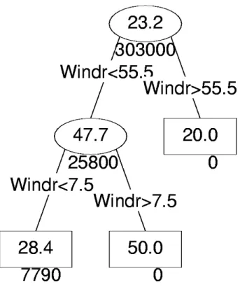
Clearly, the relationship between concentrations X and meteorology is simple and highly non-linear. Below we estimate a Regression Tree for X and the 12 predictors. The result is shown in Figure 1.

Figures within ellipses (nodes) or rectangular boxes (final nodes or leaves) represent averages of the concentrations falling under meteo conditions described above the nodes. Figures beneath the nodes are deviances, i.e. the sum of squared deviations of concentrations and the average of all concentrations falling in that node. If the sum of deviances in the leaves is much lower than the deviance in the highest node in the tree, we have made great improvement by adding meteorological factors.

From the Regression Tree in Figure 1 we see that the tree algorithm identified the right variable (Windr) to make splits for: wind direction. Furthermore, the values found for the wind sector [5.0,55.0] degrees are reasonably accurate: [7.5,55.5] degrees. Finally, if wind direction is found in the sector [7.5,55.5], concentrations are perfectly predicted: 50 µg/m3 (deviance equals zero). The same holds for wind directions > 55.5: 20 µg/m3. If wind directions are < 7.5 degrees, predictions are slight to high: 28.4 µg/m3.

(19)

Figure 1 Regression Tree for a hypothetical pollutant X, with increased concentrations for wind directions from 5 to 55 degrees.

Figures in the ellipses (nodes) represent the average of all concentrations falling under a specific meteo condition and mentioned above the node. Rectangular boxes or final nodes are called the leaves of the tree. The figures beneath nodes and leaves are deviances, i.e. the sum of squared deviations of concentrations in that node/leaf and the average of concentrations in that node/leaf. The splitting process depends on the reduction of the initial deviance (here 303,000 [µg/m3]2) to a much smaller deviance. The sum of deviances in the leaves accounts for: 7790 + 0 + 0= 7790 [µg/m3]2.

(20)

For the exact definition of terms such as ‘regression tree predictions’, ‘deviance’ and ‘predictive power’, we need some formal definitions. These are taken from the basic book on regression trees by Breiman et al. (1984). We will use these definitions in §2.3 and §2.7 (yellow text blocks).

Definitions I

As mentioned above, for estimating a Regression Tree we have a response variable yi

(concentration of some pollutant) and m predictor variables xi = (x1,i,x2,i, … ,xm,i ). In this

report xi will consist of a set of m meteorological variables. The pointer i may be expressed in

days, as in Figure 1, or in months, as in Chapter 5.

Suppose all days or months fall into J classes (the leaves of the tree). We name these classes 1,2, …, J. The estimated Regression Tree (RT) defines a classifier or classification rule c(xi),

which is defined on all xi , i =1, 2, … , N. The function c(xi) is equal to one of the numbers

1,2, … , J.

Another way of looking at the classifier c is to define Aj , the subset of all xi on which c(xi) =

j:

Aj = { xi c(xi) = j } (1)

The sets Aj, j = 1, 2, … , J are all disjunct and the unity of all sets Aj spans exactly all the N

(21)

2.2 Pruning

Trees with too many nodes will over-fit our data. In fact, we could construct a tree with as many nodes as days or months we have. The fit to the data will be very good. However, such a tree does not serve our goal of finding parsimonious models (criterion (a) in section 1.4). Therefore we have to look for an analogue of variable selection in Multiple Regression analysis.

The established methodology is tree cost-complexity pruning, first introduced by Breiman et al. (1984). They considered rooted subtrees of the tree T grown using the construction algorithm, i.e. the possible result of snipping off terminal subtrees on T. The pruning process chooses one of the rooted subtrees. Let Ri be a measure evaluated at the leaves, such as the

deviance (compare equation (3)), and let R be the value for the tree, the sum over the leaves of Ri. Let the size of the tree be the number of leaves.

By pruning Regression Trees, we try to find an optimal balance between the fit to the data and the principle of parsimony (criterion (a) in Section 1.4). To this end the full tree is pruned to a great number of subtrees and evaluated as for minimization of the so-called cost-complexity measure. Photo: H. Visser

(22)

Then, Breiman et al. showed that the set of rooted subtrees of T which minimize the cost-complexity measure:

Rα = R + α . size

is itself nested. In other words, as we increase α, we can obtain optimal trees through a sequence of snip operations on the current tree (just like pruning a real tree). For details and proofs see Ripley (1996).

The best way of pruning is using an independent test set for validation. We can now predict on that set and compute the deviance versus α for the pruned trees. Since this α will often have a minimum, and we can choose the smallest tree of which the deviance is close to the minimum. If no validation set is available, we can make one by splitting the training set. Suppose we split the training set into 10 (roughly) equally sized parts. We can then use 9 to grow the tree and the 10th to test it. This can be done in 10 ways and we can average the results. This procedure is followed in the software we have implemented in S-PLUS. Note that as ten trees must be grown, the process can be slow, and that the averaging is done for fixed α and not for fixed tree size.

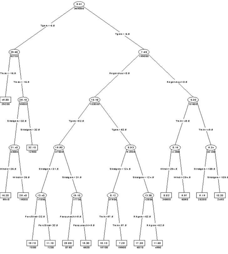
We give an example for SO2 concentrations at Posterholt station in the Netherlands.

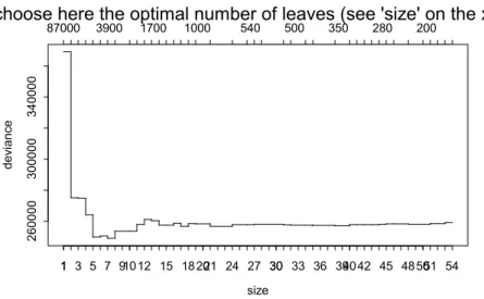
Concentrations consist of daily averages over the 1989 – 2001 period. The Regression Tree is shown in Figure 2. An example of a cross-validation plot for pruning is given in Figure 3A. The optimal tree size has been computed (values lower x-axis) for a series of α values (on upper x-axis). The values are averages of the ten-fold cross-validation procedure described above. The values on the y-axis are the deviances over all leaves of the selected trees. The graph has a clear minimum around six leaves. Thus, we decide to prune our full tree back to one with six leaves. The result is shown in Figure 3B.

(23)

Figure 2 Regression tree for daily SO2 concentrations measured at station Posterholt in

(24)

Figure 3A Cross-validation plot for pruning the tree from Figure 2. Minimum is around tree size 6.

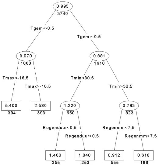
Figure 3B Pruned tree for daily SO2 concentrations at Posterholt. Temperature variables

Tgem, Tmax and Tmin are expressed in 0.1 ˚C. Variable Regenduur stands for rain duration (in hours).

size dev ianc e 260000 300000 340000 1 10 20 30 40 50 87000 3900 1700 1000 540 500 350 280 200

choose here the optimal number of leaves (see 'size' on the x-as)

(25)

Given an optimal pruned tree we can calculate daily or monthly predictions for concentrations by averaging all concentrations that fall in a certain meteo class (leaf). Therefore if we have meteo conditions which fall in that meteo class, our prediction is simply the leaf average. Thus we have as many prediction values as leaves. The formal definitions are given below.

Definitions II

Given an estimated tree with m leaves (or meteo classes), we want to make a single prediction for days or months, with meteo conditions applying to a specific leaf j. On the basis of the definitions in Section 2.1., the classification rule c puts each daily concentration in one of the meteo classes: 1,2, … , J. We can now define an RT prediction for all concentrations yi falling in meteo class j. Normally, the arithmetic mean is taken for all

concentrations falling in class j. Other values could be the median or the modus. In this report we will take the arithmetic mean.

Thus, the prediction ŷi,j ≡ µj for a concentration on day or month i, belonging to class j, is:

å

= = } ) ( | { 1 j x c i i j j i y N µ (2)

where Nj is the number of cases in class j.

The deviance, Dj, is a measure of the variation of concentrations falling in class j. It is defined

as:

å

₌ − = } ) ( | { 2 ) ( j x c i j i j i y D _µ (3)

The predictions µj are given in Figure 1 within the ellipses and boxes, while the

corresponding deviance is given below each ellipse or box.

As a general notation we will denote the predictor function by ‘d’. Thus, for each concentration yi we obtain the prediction ŷi = d(xi ), with ŷi one of the numbers µ1, µ2, … , µJ.

The variance of a specific prediction µj simply follows from the deviance (3): var(µj) = Dj/Nj.

(26)

We will now follow the SO2 example from the preceding sections. The daily concentrations

yi are plotted in Figure 4 against the predictions ŷi. Because we have a classifier with six

meteo classes, we have six values on the y-axis. These six values are identical to those given in the leaf boxes in Figure 3.

In interpreting the pruned in Figure 3B, we expect very high concentrations (45.8 µg/m3) if daily averaged temperatures are below –0.65 ˚C and maximum daily temperatures are below 1.65 ˚C. This meteo class is typically a measure for winter smog conditions. We expect the lowest SO2 concentrations (5.34 µg/m3) if daily temperatures are above –0.65 °C and rain

duration is over 0.5 hour and the minimum daily temperature is above 4.95 ˚C.

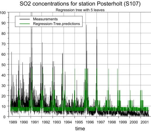
Figure 5 shows the concentrations and corresponding predictions as a time-series plot.

(27)

Figure 4 Scatterplot of daily SO2 concentrations for Posterholt station (x-axis)

measured against RT predictions.

Figure 5 Daily SO2 concentrations for Posterholt station with RT predictions.

Raw daily values of S107

RT pr edi ct ions f or S107 0 20 40 60 80 100 10 20 30 40

Original daily data against RT predictions

1989 1990 1991 1992 1993 1994 1995 1996 1997 1998 1999 2000 2001 time 0 10 20 30 40 50 60 70 80 90 100

SO2 concentrations for station Posterholt (S107) Regression tree with 5 leaves

Measurements

(28)

2.4 Predictive power in relation to rival models

To compare two alternative models for the same concentration data, we need a measure for prediction accuracy. Here, a rival model could be a regression tree with more or less nodes than the current estimated tree. A rival model could also be a model following a different statistical approach. Examples are the overall-mean predictor, the naive or persistence predictor and the Multiple Regression predictor. The overall-mean predictor uses the overall mean of all concentrations as a constant prediction for all new cases (days or months). The naive predictor uses the value of the preceding day or month as a predictor for the following day or month.

In the following text box we will define simple indices to evaluate the predictive power of a specific estimated tree, relative to the three rival models mentioned above. All indices are based on quadratic prediction errors.

Definitions III

Breiman et al. (1984) defines the following mean squared error RRT*(d) for a Regression

Tree (RT) with prediction rule d:

2 1 * ₍ ₎ 1 _[ ₍ _)]

å

= − = N i i RT y d x N d R i (4)

The asterisk is used to denote the fact that RRT is estimated on the data. Another well-known

measure for prediction performance is the minimum absolute deviation criterion (MAD). This criterion is less sensitive to outliers. However, throughout this report we will use only the criterion defined in (4).

In a similar manner we may define mean squared errors for rival models. In our approach we routinely estimate three rival models: the overall mean predictor, the naive predictor and the Multiple Regression predictor. The overall mean predictor simply uses the overall mean of the N concentrations (µ) as prediction for all days or months yi. We denote its mean squared

error by Rµ*. The naive predictor is also known as the persistence predictor and for each

concentration yi simply uses the concentration of the preceding day, thus yi-1. We will denote

its mean squared error by Rnaive*. The third model is the well-known Multiple Regression

model estimated on the same data set using the same meteorological predictor set xi. Its mean

(29)

From the mean squared errors given above we define the performance of our RT model relative to that of these three rival model as:

* * *₍ ₎ ( ) µ µ _R d R d RE ₌ RT _(5a) * * * ₍ ₎ ( ) naive RT naive R d R d RE ₌ (5b) * * * ₍ ₎ ( ) MR RT MR _R d R d RE = (5c)

We also express these relative prediction measures in percentages to express the improvement by using the RT model against one of the rival models:

(%) 100 * )] ( 1 [ ) ( * * _d _RE _d P_µ = − _µ (6a) (%) 100 * )] ( 1 [ ) ( * * _d _RE _d P_naive = − _naive (6b) (%) 100 * )] ( 1 [ ) ( * * _d _RE _d P_MR = − _MR (6c)

We note that in linear regression applications, the term 1 – RE*µ(d) is called the variance

explained by d. And the sample correlation, expressed as percentage, would be equal to P*µ(d). However, in general, RRT*(d) in equation (4) is not a variance; it does not make sense

to refer to it as ‘the proportion of variance explained’. The same holds for the squared correlation.

(30)

As an example we give the indices defined above for the SO2 regression tree shown in Figure

3. We find for this tree the following values: RRT*(d) = 53, Rµ* = 81 and Rnaive* = 41

[µg/m3]2. Now, the relative indices are REµ*(d) = 0.65, REnaive*(d) = 1.28, Pµ*(d) = 35% and

Pnaive*(d) = -28%.

Clearly, the RT predictions are better than the overall-mean predictor (35%). However, the RT predictions are 28% worse than those by the naive or persistence predictor. This indicates that we have to look for better trees to outperform this rival model (compare results in §2.8).

For the model shown in Figures 3B and 5, Regression Tree predictions are 28% worse than those made by the naive or persistence predictor (today’s prediction is yesterday’s value).

(31)

2.5 Transformation of concentrations prior to analysis

In time-series analysis it is good practice to check the data for trend and time-dependent variability (heteroscedasticity). By the latter we mean that the variability of concentrations may depend on the actual average level. Heteroscedasticity is tested through Range-Mean plots (compare to Figure 10). The most common way of removing heteroscedasticity is by applying a log-transformation prior to the estimation of a regression tree. Regression Tree predictions can be transformed back to the original scale by taking exponentials.

In Regression Tree analysis a trend is not part of the set of predictors x. If we were to add a linear trend to the set x, the Regression Tree procedure would split our time-series into a number of consecutive blocks over time (highest nodes in the tree). Then, for each block the dependence on meteorology will be accounted for (lower nodes in the tree). In this way, the number of days or months on which to estimate the actual meteo-related tree is reduced considerably. For this reason, we did not consider the addition of a trend to x 1).

However, for estimating an RT, a particular time series should have stationary characteristics. Stationarity in time-series analysis means that:

• the true (local) mean of a series is time-independent. E.g., a series may not contain a long-term trend;

• the correlation structure is time-invariant. E.g., a stationary time series has a variance which is invariant (homoscedastic) over time.

As an alternative, we remove a clear trend in the data, if necessary, and analyse the trend-corrected data by Regression Tree analysis. Regression Tree predictions and meteo-trend-corrected concentrations (compare §2.7) are transformed back to the original scale by using the inverse transformation.

Of course, there is a ‘grey area’, where it is not clear if we should remove the trend or not. In these cases it is advisable to estimate a Regression Tree to both untransformed and transformed concentrations, and to check for differences between the two.

We have implemented three transformations in the ART software (Chapter 3):

yt’ = log (yt + b) (7)

with ‘b’ a constant, such that (yt + b) is positive for all time steps t. This transformation

stabilizes variability over time.

___________________________________________________________________________

1) _{We note that the approach of adding a linear trend to the set of predictors also has an advantage.} Because Regression Trees are estimated for two or more sub-periods, we can test the stability of the tree as a function of time.

(32)

If significant trends over time exist, we apply one of the following transformations:

yt’ = yt - trendt (8a)

or

yt’ = yt / trendt (8b)

Transformation (8b) has a stabilizing effect on the variability of the concentrations.

The trends in equations (8a) and (8b) are satisfactorily estimated by an n-degree polynomial yt = a0 + a1t + … + antn. As for concentration data, n has a maximal value of 3. To ensure

stable estimates of the polynomial, we use the function POLY from S-PLUS.

Another important group of transformations is formed by the Box-Cox transformations, which have advantages in transforming data to normality. However, a disadvantage is the interpretation of the transformed concentrations. We decided not to implement this group of transformations.

As an example we have transformed the Posterholt SO2 data by using transformation (8b).

This transformation removes the trend, and the trend dependence of the variance, at the same time. Now the tree shown in Figure 3 for untransformed data changes into the tree shown in Figure 6. Comparing Figures 3 and 6 we see that the main variables used for splitting are similar. However, the values for splitting differ between trees. The splitting order is also different. We conclude that trend removal to be an essential first step in the analysis here.

(33)

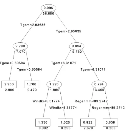
Figure 6 Regression tree for SO2 concentrations at Posterholt.

Before estimating the tree, transformation (8b) was used to remove the trend from the data and to stabilize the variance over time. Transformed concentrations vary at around 1.0. Splitting variables for average daily temperature (Tgem), maximum daily temperature (Tmax) and minimum daily temperature (Tmin) are expressed in tenths of ˚C. Rainfall (Regenmm) is expressed in tenths of mm, and rainfall duration (Regenduur) in hours.

(34)

2.6 Validation and stability of trees

As well as providing a good fit within the relevant sample, our optimal pruned regression tree, and in fact any model, should give a good fit outside the data (compare criterion (e) in section 1.4). Therefore it is good practice to use the data available as a so-called trainingset, and to predict concentrations on other independent data; this is called the testset.

Criteria to evaluate the prediction performance of the tree to a testset or a trainingset, have been given in section 2.4. Now RT predictions on the testset data are generated by using the estimated tree, estimated in the trainingset, in combination with the explanatory variables available in the testset. In this way our predictions are not based on any information on concentrations falling in the testset. For the overall-mean predictor we use the mean for all concentrations in the trainingset as the predictor for the concentrations in the testset.

An example of cross validation is given in Table 1. Here, we evaluate the indices from equations (6) and (7) for:

• all daily SO2 concentrations from Posterholt station (second column);

• all data minus the data of 1994 (third column); • all concentrations occurring in 1994 (fourth column); • all data minus the data for 2000 (fifth column); • all concentrations occurring in 2000 (sixth column).

The table shows predictions during the testset periods 1994 and 2000 to be very good. Both indices Pµ*(d) and Pnaive*(d) in the testsets are higher than the corresponding values in the

trainingset (compare percentages fourth row).

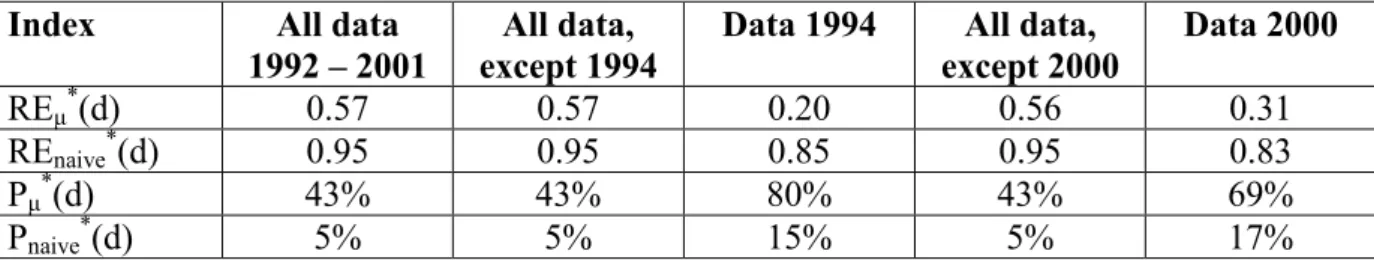
Table 1 Indices from equations (5) and (6) for all data (1992-2001), all data except the days in 1994 (trainingset), all data in 1994 (corresponding testset), all data except the days in 2000 (trainingsset) and all data in 2000 (corresponding testset).

Index All data

1992 – 2001 except 1994All data, Data 1994 except 2000All data, Data 2000

REµ*(d) 0.57 0.57 0.20 0.56 0.31

REnaive*(d) 0.95 0.95 0.85 0.95 0.83

Pµ*(d) 43% 43% 80% 43% 69%

Pnaive*(d) 5% 5% 15% 5% 17%

The stability of an estimated tree could be low for two reasons. First, the tree may contain too many nodes. In this situation many explanatory variables are able to lower the overall deviance of the tree in the same small manner; furthermore, we can estimate a number of equivalent trees.

(35)

Multiple Regression analysis this problem is called multi-collinearity and in the filter theory the filter is said to be not observable. Lack of observability means that the output of a filter is not uniquely determined by its input variables.

In Regression Tree analysis multicollinearity manifests itself in the choice of specific variable xi to make a certain split. Reduction in deviance is reached for multiple x-variables if they are

highly correlated. An example of multicollinearity in the examples throughout this report is shown in the variables:

• daily averaged temperature (variable Tgem); • daily maximum temperature (variable Tmax);

• daily minimum temperature (variable Tmin), and to a lesser extent; • global radiation.

Scatterplots for Tgem, Tmax and Tmin are given in Figure 9.

Are there solutions to the problem of multicollinearity? The answer is simply no. Statistics is not able to provide the exact unique relationships between some variables yi, x1,i and x2,i if x1,i

and x2,i are highly correlated. Information other than that based on statistical inferences

should answer which variable should be coupled to yi.

In most cases the instability of Regression Trees is caused by multicollinearity, i.e. high correlation among the predictors x. To test for stability, we may compute the correlation matrix of all predictors. A cross validation on the final tree will reveal instability as well.

(36)

We note that some researchers have applied a principal component transformation to all explanatory variables, making a new set of variables x’ (principal components) that are uncorrelated with each other. The modelling is then performed between yi and these

principal components (e.g. Fritts, 1976). However, a serious drawback of this approach is that the selection-of-variables process (MR analysis) or the building of a tree (RT analysis) is performed on xi’ variables which have no clear physical interpretation. Therefore we do not

advocate this approach.

2.7 Meteorological correction

We consider here two methods for calculating meteo-corrected concentrations on the basis of an optimally pruned tree. The first method has been proposed by Stoeckenius (1991). A meteo-corrected annual value or annual percentiles can be calculated with this method on the basis of frequency of leaves within a certain year relative to the frequency of the leaves for all years. The method of Stoeckenius has been described in detail in Dekkers and Noordijk (1997). In Noordijk and Visser (in prep.) refinements will be given to the method of Stoeckenius.

The second method has been described at the end of §1.3. The method gives meteo-corrected value for each day or month (this is not the case for the method of Stoeckenius). Annual averages or percentiles are simply calculated on these meteo-corrected days.

Throughout this report we will apply the latter method. An evaluation of both correction methods will be given in Noordijk and Visser (in prep.).

(37)

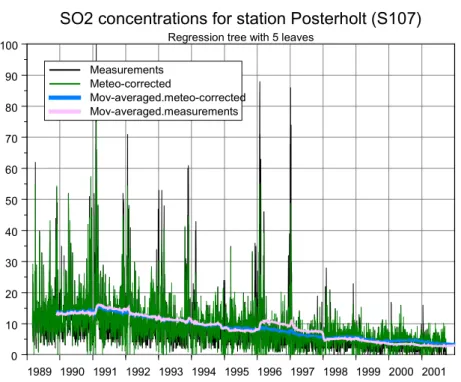
predictions, based on the optimal pruned tree shown in Figure 6. The graph shows much overlap between measurements and meteo-corrected data, indicating that not much of the daily behaviour of SO2 can be attributed to meteorological variations.

Figure 7 Concentrations (black curve) and RT predictions (green curve) for daily SO2

concentrations at Posterholt.

The pink curve shows the moving average of concentrations using a window of 365 days, while the blue curve show the same for the meteo-corrected daily data. 1989 1990 1991 1992 1993 1994 1995 1996 1997 1998 1999 2000 2001 time 0 10 20 30 40 50 60 70 80 90 100

SO2 concentrations for station Posterholt (S107)

Regression tree with 5 leaves Measurements

Meteo-corrected

Mov-averaged.meteo-corrected Mov-averaged.measurements

(38)

2.8 Influence of sampling time

Finding rival models to a certain Regression Tree should not be limited to models based on other statistical principles. One should also check the sampling time of the measurements, yi.

If one analyses concentrations on the basis of hourly data, one will find mainly local meteorological conditions governing daily variations. If one uses daily averaged concentrations, one will find mainly meteo variables governing variation over the Netherlands within weeks. If one uses monthly averaged data, one will mainly find the meteo variables governing the annual cycle, on the scale of NW-Europe. Therefore it makes sense to check the sampling time when modelling concentrations.

As an example we have modelled the SO2 concentrations for the Posterholt station using

monthly averaged SO2 concentrations and the transformation (8b). The Regression Tree is

shown in Figure 8A and the corresponding time-series plot with concentrations and monthly RT predictions in Figure 8B.

Figure 8A Regression tree for monthly SO2 concentrations at Posterholt.

Before estimating the tree, transformation (4c) was used to remove the trend from the data and to stabilize the variance over time. Transformed concentrations vary at around 1.0. Temperatures (Tgem) are expressed in ˚C, total monthly precipitation (Regenmm) in mm, and wind speed (Windkr) in m/sec.

(39)

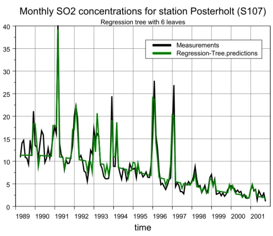
Figure 8B Concentrations (black curve) and RT predictions (green curve) for monthly SO2 concentrations at Posterholt. The model is based on the Regression Tree

from Figure 8A.

The difference in the RT based on daily and monthly data is clearly shown by the great differences in predictive power, as shown in Table 2. We can conclude from Table 2 that an RT based on monthly SO2 data is much better in describing large-scale meteorological

conditions similar to those reflected in inter-annual variation of concentrations. A similar result is found for PM10 concentrations (Chapter 5).

Table 2 Indices from equations (5) and (6) for daily and monthly SO2 concentrations.

Data are for Posterholt station.

Index Daily data

1992 – 2001 Monthly data1992- 2001 REµ*(d) 0.57 0.20 REnaive*(d) 0.95 0.17 Pµ*(d) 43% 80% Pnaive*(d) 5% 83% 1989 1990 1991 1992 1993 1994 1995 1996 1997 1998 1999 2000 2001 time 0 5 10 15 20 25 30 35 40

Monthly SO2 concentrations for station Posterholt (S107) Regression tree with 6 leaves

Measurements

(40)

We note that by changing the sampling time from days to months, difficulties arise for wind direction. A monthly averaged wind direction has no meaning. For this reason we have added six dummy variables, each variable for one wind-direction sector of 60 degrees. Monthly averages of these variables now give the fraction of days in a month with wind direction in that particular wind sector. The sum of these monthly fractions is held to be 1.0.

2.9 Procedure in eight steps

In this document we aim to describe refinements of the approach of Dekkers and Noordijk (1997). Basically, the method proposed here consists of an eight-step procedure:

1. Check for outliers with descriptive statistics on the data. Explore the relationships between variables by scatter matrices.

2. Check to see if the original data should be transformed before RT analysis (e.g. to eliminate trends).

3. Classify the meteorological conditions. To this end an initial Regression Tree is estimated and then pruned to give the final Regression Tree.

4. Calculate leaf numbers, leaf predictions and meteo-corrected concentrations.

5. Validate the optimal Regression Tree by omitting certain years of data. By predicting these omitted data and comparing predictions with the real concentrations, an impression is gained of the predictive power and the stability (robustness) of the optimal Regression Tree (the principle of cross validation).

6. Make diagnostic checks on residuals and leaf frequencies for the optimal tree. 7. Visually inspect concentrations, predictions and meteo-corrected concentrations.

8. Compare variables in the optimal Regression Tree as well the predictive power of the tree with those found by estimating a Multiple Regression model on exactly the same data. As a final step we may fit a low-pass filter through the meteo-corrected concentrations, which allows the estimate of 90% confidence limits. In general, the fit is based on a second-order polynomial (a 'parabola fit'). The filter separates an emission-related concentration trend and noise. However, it assumes consistency in the measurements and a smooth change in emissions (no sudden changes). Because of this assumption we name this step ‘optional’.

(41)

The Regression Tree approach also has limitations. We recall two drawbacks here of importance for the interpretation of the Regression Tree results (compare §2.6):

• highly correlated predictors induce instability in tree estimates;

• if both response variable yt and selected predictors xi,t contain long-term trends, the

meteo-correction procedure could become sub-optimal. The method cannot uniquely distinguish between emission-induced changes in concentration and meteorologically-induced changes.

We provided guidelines in §2.6 to detect potential instability of tree estimates by the reasons mentioned above. However, if such instabilities occur, results should be presented with care.

(42)

(43)

3. ART software

3.1 S-PLUS functions and scripts

A state-of–the-art software library on CART analysis is available within S-PLUS. A general description on S-PLUS for RIVM is given by Dekkers (2001). The implementation of Regression Tree routines is described in S-PLUS ( 2000) and Venables and Ripley (1997). We have extended the RT software library of S-PLUS with a number of scripts and functions to enable the analyses and tests described in the preceding chapter. We have named this software tool ART ( Air pollution by Regression Trees).

ART consists of a number of S-PLUS scripts and routines. In the S-PLUS script (Appendix A) a number of these functions are named. Details on these functions and additional scripts will be given in Visser (in prep.). In Chapter 4 we will give a step-by-step example of the use of ART based on the script given in Appendix A.

The Regression Tree methodology is implemented in ART (Air pollution and Regression Trees). This software is based on S-PLUS routines. Photo: H. Visser

(44)

3.2 Preparing data prior to analysis

Because the ART software is implemented within S-PLUS, one has to import air pollution data and meteorology into S-PLUS. Data structures in S-PLUS are called dataframes. In Visser (in prep.) a detailed description is given on how to import air pollution data from a number of stations into one data frame. A script is also given for the import of meteorology and divided into five regions over the Netherlands, leading to the generation of 5 data frames. As a final step, all air pollution stations are coupled to the meteo-region data frame to which they correspond, leading to 5 additional data frames. ART analyses are performed on these final data frames.

(45)

4. Regression Tree analysis step by step

In this chapter we will demonstrate the estimation of a proper Regression Tree with corresponding concentration predictions and meteo correction as a 7-step procedure. For illustrative purposes we have made a simulated example (Appendix G in Visser, 2002; the yellow area).

Here, a data frame, Pseudo5, is generated with a dependent variable yt = Tgem/10, i.e. our

air pollution component is 100% linear coupled with air temperature (divided by 10 to obtain temperature in oC). Explanatory variables are:

1. Tgem daily averaged temperature in tenths ºC 2. Tmin minimum hourly temperature in tenths ºC 3. Tmax maximum hourly temperature in tenths ºC 4. RHgem relative humidity in %

5. Regenmm amount of precipitation in tenths mm 6. Pgem air pressure in mbar

7. Stralgem radiation in J

8. PercStral percentage radiation 9. Windr wind direction in degrees 10. Windkr wind speed in m/sec

11. Pasqudag Pasquill stability class for daytime conditions 12. Pasqunacht Pasquill stability class for night-time conditions

This example is also interesting because we can see how RTA handles (perfect) linear relations between yt, and one or more explanatory variables. This is typically a situation

where Multiple Regression (MR) will find the right relationship because MR estimates linear relations by definition.

Furthermore, we know the perfect prediction for each day, Tgemt/10, in advance. We also

know the meteo-corrected daily value of ‘Index’ in advance. Because all variations in the series ‘Index’ are due to meteorological factors, the meteo-corrected ‘Index’ should be constant over time. This value is the average value of the variable Tgem/10 over all 3653 days in the period 1992-2001: 10.3 ºC. How well will our Regression Tree estimation procedure reconstruct these values?

The eight-step procedure is given in Appendix A as an S-PLUS script. In the following sections we will describe these steps using the data from data frame Pseudo5.

(46)

4.1 Step 1: looking at the data

We block aa.dat <- Pseudo5[-1:-365,] (yellow area in Appendix A) in the SPLUS script RTAonPseudoseries. In doing this we copy our dataframe, Pseudo5 to the general dataframe aa.dat. The addition [-1:-365,] means omitting the first 365 days in the dataframe (this is the year 1991). Now the analysis covers the years 1992 through 2001, where N = 3653 days.

Second, we block m<- …. , to generate general statistics for each of the variables in our dataframe. This is for a general check on the input data. How many data are missing and are there specific outliers?

Third, we block guiplot… to generate a scatter-plot matrix between all variables involved. The first scatter-plot matrix for Pseudo5 is given in Figure 9. Here, we see the perfect linear relation between variable Index (our dependent variable yt) and explanatory variable Tgem.

yt is also highly correlated to variables Tmint and Tmaxt, which reflects the high correlation

between daily averaged, daily maximum and daily minimum temperatures.

Figure 9 Scatter-plot matrix for eight variables from Pseudo5. Variable ‘Index’ is the dependent variable. Time t is in days and runs from 1992 to 2001 (N= 3653).

Index 00E+00209E-014 00E+002 00E+002 00E+002 -1000 100 200 300 0 100 200 300 9800 10000 10200 10400 -10 0 10 20 30

-1.00000E+002-1.42109E-0141.00000E+0022.00000E+0023.00000E+002

Tgem Tmin -200-100 0 100200 -1000 100200300 Tmax RHgem 40 60 80 100 0 100 200 300 Regenmm Regenduur 0 50100150200 -10 0 10 20 30 9800100001020010400 -200 -100 0 100 200 40 60 80 100 0 50 100 150 200 Pgem

(47)

variables mentioned above. We note here that the string vector luvo may contain any subset from the 12 explanatory variables.

4.2 Step 2: transformation of concentrations

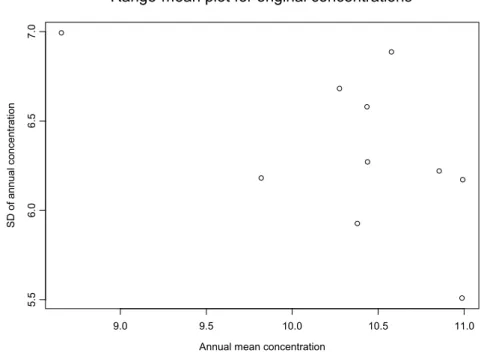
Step 2 is marked in the colour green in Appendix A. In this step we verify if data should be transformed before performing a Regression Tree analysis. See §2.6 for details. Figure 10 shows the range-mean plot. The points lie more or less on a horizontal line, indicating that the variance for each year does not depend on the corresponding annual mean concentration.

Figure 10 Range-mean plot for variable Pseudo5.

A time-series plot with the long-term trend is given in Figure 11. The graph confirms our findings from Figure 10: no transformation is needed for this example.

Annual mean concentration

S D of annual concentration 9.0 9.5 10.0 10.5 11.0 5. 56 .0 6. 57 .0

(48)

Figure 11 Time-series plot for Pseudo5 with estimated trend (green line). Time C oncentration 0 1000 2000 3000 -10 0 10 20

(49)

4.3 Step 3: initial Regression Tree and pruning

Step 3 is marked in the colour blue in Appendix A. In this step we block f.RTAnew (aa.dat, ”Pseudo5”, ”Index”, luvo, 1, 80, 40). The second argument, Pseudo5, is used as a unique identification of files and graphs. The same holds for Index, which, at the same time, is the name of the yt variable. The raw initial tree is given in Figure 12. This graph is automatically

displayed by S-PLUS.

Figure 12 Raw initial tree with identification Pseudo5.Index.met1.

From Figure 12 we see that the trees contains eight leaves and all splits are done using variable Tgem. Note that the variable Tgem has a unity of tenths of ºC, so the values should be divided by 10 to obtain the value in ºC.

Second, we obtain a menu for choosing a lower number of leaves, used for pruning of the initial tree. We can decide to prune on the basis of the cross-validation plot given in Figure 13, which is also automatically displayed by S-PLUS. We see from Figure 3 that the number of eight leaves is optimal and, therefore, we decide to keep the full tree with eight leaves (in real applications we will choose a number much lower than the maximum number of leaves found in the initial raw tree).

The final tree, which in our case is equal to the raw initial tree, is saved in a Postscript file c:RTAdataOri/Pseudo5.Index.met1. By clicking this file, GSview will display the final tree in a format more elegant than that shown in Figure 12. The tree can be blocked by choosing Edit and Copy C in GSview. Then it can be displayed in a Word file by typing Cntrl V. See Figure 14 for this final tree.

All calculated results are sent to the screen and automatically printed on the standard black-and-white printer. | Tgem<103.5 Tgem<38.5 Tgem<-5.5 Tgem<71.5 Tgem<162.5 Tgem<133.5 Tgem<199.5 -3.058 1.949 5.610 8.732 11.840 14.810 17.840 22.020

(50)

If a transformation is chosen (variable Trans in the argument list of function f.RTAnew set to ‘2’ or ‘3’), S-PLUS will generate plots of the original data with the estimated trend, as well as a plot of the trended data. Now the Regression Trees will be estimated on these de-trended concentrations. If the estimated trend is too inflexible, a more flexible trend may be estimated by setting the last argument from f.RTAnew to a higher number (a polynomial with a higher order is chosen).

Figure 13 Cross-validation plot for finding the optimal number of leaves (plotted on the x-axis). The curve has no clear minimum. Therefore, we choose eight as the optimal number of leaves.

size deviance 0 40000 80000 120000 2 4 6 8 99000 17000 14000 2900 2900 2600 2400 -Inf

choose here the optimal number of leaves (see 'size' on the x-as)