Evaluating and Modeling the Performance and Energy Efficiency of Multi-Core Turbo-Boost

(1)

Energy Efficiency of Multi-Core Turbo-Boost

Evaluating and Modeling the Performance and

Academic year 2019-2020

Master of Science in Computer Science Engineering

Master's dissertation submitted in order to obtain the academic degree of

Supervisor: Prof. dr. ir. Lieven Eeckhout

Student number: 01500322

Jaime Roelandts

(2)

(3)

Energy Efficiency of Multi-Core Turbo-Boost

Evaluating and Modeling the Performance and

Academic year 2019-2020

Master of Science in Computer Science Engineering

Master's dissertation submitted in order to obtain the academic degree of

Supervisor: Prof. dr. ir. Lieven Eeckhout

Jaime Roelandts

(4)

Preface

The author(s) gives (give) permission this master dissertation available for consultation and to copy parts of this master dissertation for personal use.

In all cases of other use, the copyright terms have to be respected, in particular with regard to the obligation to state explicitly the source when quoting results from this master dissertation. 31/05/2020

(5)

Acknowledgment

Last year, when I chose the subject for this master dissertation, an adventure began. Fast forward one year and here we are, at the end of this incredible adventure, with a complete master dissertation. However, this would not have been possible without the help of my supervisor. For this reason, I would like to say thank you to Prof. Dr. ir. Lieven Eeckhout for providing the weekly meetings, the valuable feedback and most importantly the valuable knowledge. All that help steered me in the right direction to conduct research and to deliver this master dissertation. I would also like to express my gratitude towards Dr. ir. Almutaz Adileh, who supervised the project and helped me at the start of the year.

Lastly, I would like to say thank you to all the people who provided me with corrections, feedback and support during this master dissertation.

(6)

Abstract

Evaluating and Modeling the Performance and Energy

Efficiency of Multi-Core Turbo-Boost

Jaime Roelandts

Supervisor: Prof. dr. ir. Lieven Eeckhout

Master’s dissertation submitted in order to obtain the academic degree of Master of Science in Computer Science Engineering

With the rising importance of energy consumption of processors, techniques such as Dynamic Voltage and Frequency Scaling (DVFS) were introduced [1] to reduce the power consumption by adapting the voltage and frequency depending on the needs of the processor so that high performance is provided when needed. However, processors could produce higher performance by making use of DVFS, but instead of reducing the performance, it will augment the perfor-mance for a short duration. The general name of this technique is Turbo Mode [2], which Intel implemented as Turbo Boost. This master dissertation investigates the Turbo Boost technology, in particular, the mechanism itself and the various parameters required to control the Turbo Boost mechanism. Both the conditions and effectiveness of Turbo Boost is looked into, whereby the type of workload, number of cores and temperature affect the use of Turbo Boost. Then an overview of the performance and energy of Turbo boost is provided to find ways to optimise the usage of Turbo Boost. The effect of Turbo Boost on various workloads and a varying number of cores and frequencies is assessed, whereby it is found that using the maximum number of cores will give the best performance and will be the most energy-efficient. Finally, this master dissertation shows that there is a trade-off between the performance and energy on the usage of Turbo Boost, as higher frequencies will achieve higher performance but at a superlinear increase of the energy consumption. Finally, we provide details regarding the mathematical deduction of the trade-off between performance and energy scaling, to see under which constraints the previous conclusions would hold by simulating the Turbo Boost mechanism itself.

(7)

EVALUATING AND MODELLING THE PERFORMANCE AND ENERGY EFFICIENCY OF MULTI-CORE TURBO-BOOST 2020

Evaluating and Modelling the Performance

and Energy Efficiency of Multi-Core

Turbo-Boost

Jaime Roelandts

Supervisor: prof. dr. ir. Lieven Eeckhout

Abstract—With the increasing importance of energy-efficient computing, a technique called Dy-namic Voltage and Frequency Scaling (DVFS) was introduced and implemented by major vendors [1]. That way, processors could reduce their frequency and thus their energy consumption when performance is not needed. However, performance is still an important metric for processors, which led to the introduction of Turbo Boost. Turbo Boost was created by taking the idea of DVFS and reversing its operation by raising the frequency when performance is needed [2]. This paper investigates the inner workings of Turbo Boost implemented by Intel. To find possible optimisations, the performance obtained with Turbo Boost is assessed and it is analysed which components affect Turbo Boost. Furthermore, we inspect the trade-off between the energy usage of Turbo Boost and the performance obtained from it. Finally, we provide details regarding a mathematical deduction for the speedup and energy scaling factor.

Index Terms—power-efficient computing, DVFS, In-tel Turbo Boost, computer architecture

I. INTRODUCTION

Through the years, Turbo Boost became a core component of the modern processor. Major vendors such as Intel and Advanced Micro Devices (AMD) implemented this technique on their products, with AMD calling it Turbo Core. Starting from 2008 with the first iterations of Turbo Boost [3], nowadays Intel ships their processor with the Turbo Boost 2.0 technology. They also recently announced their third generation, Turbo Boost 3.0, for some of the tenth generation processors.

Turbo Boost is a technique where the processor exceeds its nominal frequency for a short duration. This technique provides short bursts of performance for the processor. However, for reasons such as the temperature of the processor and the power consumption, the duration of Turbo Boost is meant to be kept short. On the other hand, Turbo Boost

comes with an energetic cost: due to the increase in frequency, the voltage will also increase, which results in an increase in dynamic power and thus of energy consumption.

In this paper, we will focus on Turbo Boost 2.0 implemented by Intel. The mechanism of Turbo Boost itself is looked at in detail, together with the different parameters that define the behaviour of Turbo Boost. Before that, DVFS has to be explained. Once the Turbo Boost mechanism is understood, the performance of Turbo Boost is assessed. By going over the different components that could af-fect Turbo Boost, we show that Turbo Boost can be negatively affected by the temperature of the processor. Furthermore, the impact of multiple cores running Turbo Boost is also reviewed. It is shown that there is a linear increase of performance with the frequency due to Turbo Boost across multiple cores.

Once the performance of Turbo Boost is assessed, we look into the energy consumption of processors. By varying the maximum frequency and the number of active cores, we show that it is more efficient to use the maximum number of cores possible without Turbo Boost to enhance the performance and reduce energy consumption. Turbo Boost could be used as an additional step to increase the performance, at the cost of higher energy consumption.

Finally, we show that the previous conclusions will hold if the frequency on i cores does not drop below 1

i times the frequency running on one core.

Similarly, we show that the power consumption needs to be less than i times the power consumption running on one core. In order to formulate those results mathematically, we derive some extensions from Amdahl’s law.

(8)

II. BACKGROUND

A. DVFS

Dynamic Voltage and Frequency Scaling (DVFS) is a technique that allows the processor to operate at multiple frequencies. The reason why one would want to change the frequencies dynamically, is to reduce the power consumption of the processor. Due to an increase in frequency, the voltage on the processor will also increase, so that the transistor’s switching time is shortened in order to keep up with the higher frequencies. Unfortunately, the dynamic power will increase quadratically with the voltage and linearly with the frequency. This implies that if the frequency increases, one would expect up to a third power increase of the dynamic power [1], [4]. For this reason, the frequency and voltage will scale depending on the needs of the processor, so that the processor will not consume too much when the processor is idle, but when a program is executed, the frequency and voltage will ramp up. B. Mechanism of Turbo Boost

0 20 40 60 0 20 40 60 80 100 120 EWMA PL2 PL1 Time (s) Po wer (W)

Turbo Boost mechanism

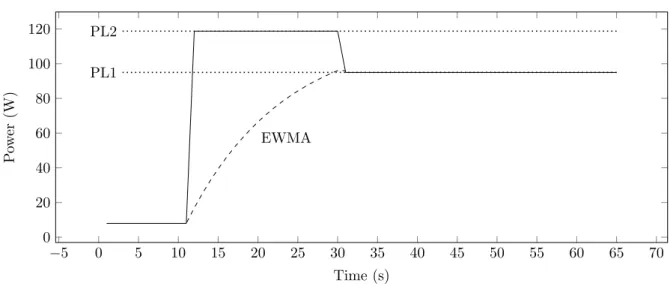
Fig. 1: An illustration of the Turbo Boost mecha-nism.

Turbo Boost builds upon the idea of DVFS. Instead of reducing the frequency and voltage when the processor is not needed, it will scale the fre-quency and voltage above the nominal frefre-quency to provide a short burst of performance [2].

In Figure 1, there is a visualisation of the Intel Turbo Boost mechanism, where the power is plotted

over time. In the Figure, the processor is idle for 11 seconds, then the processor is allowed to consume power up to the Power Limit 2 (PL2) level. Mean-while, there is an Exponential Weighted Moving Average (EWMA) that will update every timestamp by taking a weighted average of its current value and the new power value. Once the EWMA reaches the Power Limit 1 (PL1) level, the processor is forced back to consume a maximum of PL1 power.

Note that, if there is only one core running at the Turbo Boost frequency, it may be possible that the power does not exceed the PL1 level. Thus the EWMA would never reach the PL1 level and the processor could, in theory, keep the turbo frequency running forever.

The thermal design power (TDP) is defined by Intel as the average thermal power the processor should release on average. Because there is a one-to-one relationship between the power consumed and the released thermal power, the Power Limit 1 (PL1) is recommended to be set at the TDP by Intel. That way, the processor consumes on average the TDP amount of power due to the EWMA. The PL2 level on the other hand, is recommended by Intel to be set at 1.25 times the PL1 level, but can be controlled by the operating system.

There is one last parameter that controls how fast the EWMA grows. That parameter weighs the importance of the current average with the new power at that time. This is likely the parameter Tau stated by Intel, which they define as the average time the Turbo Boost may run. However, Intel does not disclose explicitly how they calculate the EWMA with that Tau parameter [5].

III. EXPERIMENTAL SETUP

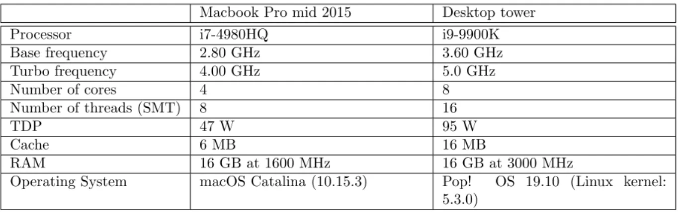
For the experiments, there are two machines on which the benchmarks were run. First of all, there is a MacBook Pro machine from mid 2015, which is a small laptop that has a limited airflow. It contains a i7-4980HQ processor, which runs at a base frequency of 2.80 GHz and a turbo frequency of 4.00 GHz; its TDP is 47 Watt. The second machine on which most benchmarks were run is a desktop computer with a i9-9900K, running at a base frequency of 3.60 GHz and a turbo boost frequency of 5.00 GHz; its TDP is 95 Watt.

There are four benchmarks on which the experi-ments are run. The first one is a compute intensive pi calculation benchmark, which uses the Leibniz approximation to approximate pi. The benchmark consists of calculating more and more values in the

(9)

series. When multiple cores are active, the number of iterations are split across the cores, making this program embarrassingly parallel.

The second benchmark is another synthetic benchmark which is more memory intensive. By creating a giant linked list where the elements point randomly to one another, the benchmark had to retrieve each value one-by-one from memory. When multiple cores are active, the chain and iterations are split between them.

The third benchmark is from the Parsec bench-mark suite, in particular the freqmine benchbench-mark [6]. Compared to the results of a synthetic bench-mark, this benchmark provides a better view of the speedup that can be expected from Turbo Boost.

Finally, the last benchmark was run to moni-tor the power consumption of Turbo Boost. That benchmark is called mprime, which is classified as a power virus because it has a torture test built-in which intends to draw as much power as possible [7].

IV. KEY FINDINGS

A. Impact of Temperature

The first key finding is the impact of high temper-atures on Turbo Boost. Intel created a firmware in order to protect the processor from overheating and damaging itself. When a processor hits a ture limit, which Intel named the junction tempera-ture, the processor will throttle the performance by reducing the frequency so that the processor’s tem-perature can cool down. However, if the processor still stays too hot, it might even shut itself down.

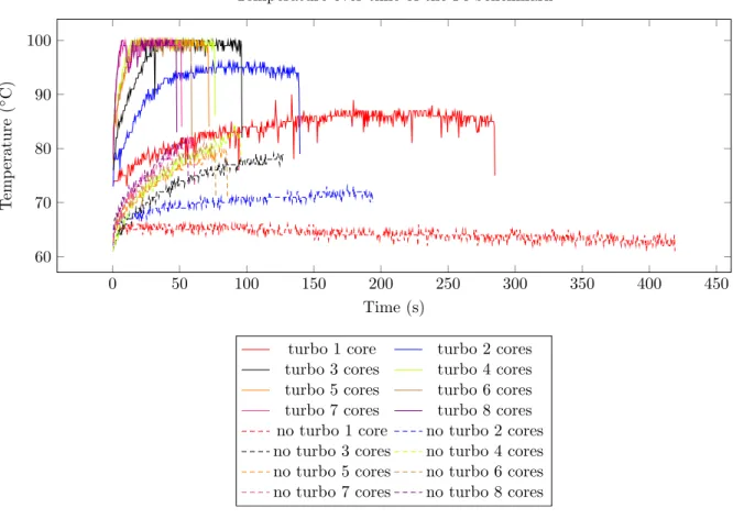
The insight regarding the temperature was ob-tained during the execution of the pi-synthetic benchmark on the MacBook Pro computer. Figure 2 illustrates the temperature of the runs with Turbo Boost for multiple numbers of active cores. It can be seen that, once the processor uses more than three cores, the junction temperature is hit. This translates to a slower increase in performance across the cores. In Table I, the speedup with respect to one core with-out Turbo Boost is shown. The relative speedup is also shown, which is the speedup obtained through turbo on the same number of cores. When looking at the relative speedup, it can be seen that once three cores are hit, the performance significantly drops, making Turbo Boost less effective.

B. Impact of the Core-Count

The number of active cores should affect Turbo Boost in theory, as seen in Section II. It would

cores turbo no turbo relative speedup 1 1.46 1.00 1.46 2 3.00 2.12 1.42 3 4.33 3.26 1.33 4 5.52 4.33 1.27 5 6.08 4.80 1.27 6 7.24 5.35 1.35 7 8.10 6.50 1.25 8 8.82 7.12 1.23 average (no SMT) 1.37 average 1.32

TABLE I: Relative speedup, where a third column has been added to calculate the relative speedup between turbo and no turbo for the same number of cores. The values rounded to three significant figures. 0 100 200 300 80 90 100 Time (s) Temperature ( ◦C)

Temperature over time of Pi Benchmark

turbo 1 core turbo 2 cores turbo 3 cores turbo 4 cores turbo 5 cores turbo 6 cores turbo 7 cores turbo 8 cores Fig. 2: Pi-calculation benchmarks for Turbo Boost runs

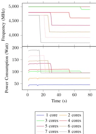
be expected that, as the number of cores increases, the power consumption increases, reducing the time in Turbo Boost. Figure 3 presents the results from the frequency and the power consumption from the Mprime benchmark. It can be seen that the duration of Turbo Boost is dependent on the number of active cores. For the highest number of cores, the

(10)

duration in Turbo Boost is reduced each time. There is an exception for the runs with one or two cores, because they both do not go over the TDP. In theory, they could keep running at the Turbo Boost frequency forever. 4,000 4,500 5,000 Frequenc y (MHz) 0 20 40 60 80 50 100 150 200 Time (s) Po wer Consumption (W att) 1 core 2 cores 3 cores 4 cores 5 cores 6 cores 7 cores 8 cores

Fig. 3: Mprime benchmark cut back to the first 80 seconds from the total 180 seconds benchmark.

What is interesting to note is that the average energy usage between the different core counts is the same with the exception of the runs with one or two cores, at about 17200 Joules for the full 180 seconds. This is as expected, since the EWMA will try to obtain the same power on average, independently from the number of cores, but the number of cores will change the power consumption.

C. Impact of the Type of Program

In order to study the impact of the type of program, the synthetic memory benchmark was run on the MacBook machine. This way, the achieved speedup could be compared against the pi bench-mark which was a synthetic compute-intensive benchmark.

The speedup achieved by the memory-intensive benchmark for one core between active and de-activated Turbo Boost was 1.30, where the pi-calculation benchmark had achieved a speedup of 1.46, which can be seen in Table I. For two cores the speedup for the memory-intensive benchmark was about 1.38 which is again smaller than the compute-intensive benchmark which achieved a speedup of 1.42. However, the pi-calculation benchmark was throttled by the temperature, preventing comparison of the results beyond two cores.

In conclusion, the type of program will affect the performance, especially if the program would have to wait for longer latencies such as hard-drive latencies or even network latencies.

D. Speedup of Turbo Boost

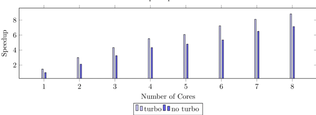
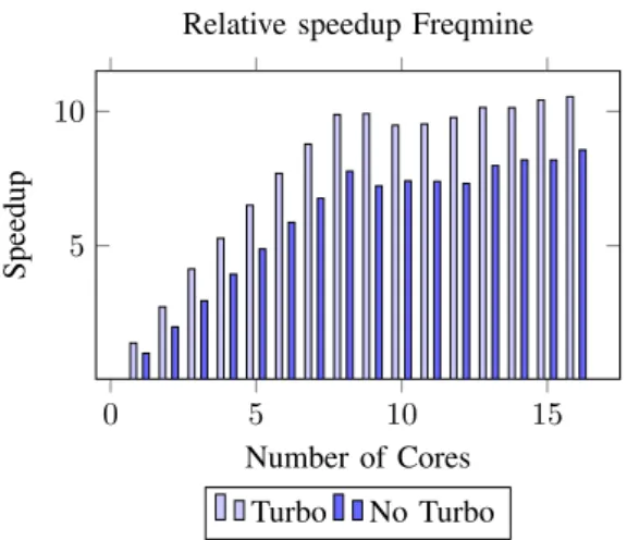
In order to obtain expected speedups which were more realistic, the Parsec benchmark was run on the i9-9900K processor to avoid any thermal throttling. Figure 4 presents the results of the speedup of the Freqmine benchmark. It can be seen in the Figure that the speedup with Turbo Boost is about a constant factor faster than the run without Turbo Boost for each number of cores. Table II contains the relative speedup for each number of active cores. It can be concluded that it stays approximately the same, with a slight decrease on the higher core counts due to lower a lower achievable Turbo Boost frequency.

When the average frequency is obtained, it is possible to calculate an approximated speedup by dividing the average frequency during Turbo Boost by the base frequency, which is 3600 MHz in this case. The calculated speedup was computed that way, as displayed in Table II. It can be seen that both the computed and measured speedup are similar, implying that the speedup will grow linearly with the increase in frequency achieved by Turbo Boost. E. The Energy Consumption of Turbo Boost

Turbo Boost uses more power due to the increased frequency, but it offers an additional speedup. In order to assess the trade-off between the energy consumption and the speedup obtained through the number of active cores and the frequency, the freqmine benchmark was executed. To be precise, it was run at multiple frequencies between Turbo Boost activated and deactivated, while varying the number of cores.

(11)

0 5 10 15 5

10

Number of Cores

Speedup

Relative speedup Freqmine

Turbo No Turbo

Fig. 4: Relative speedup between Turbo and no Turbo

cores average frequency (MHz)

calculated

speedup measuredspeedup 1 4999.88 1.39 1.38 2 5000 1.39 1.38 3 5000 1.39 1.40 4 4802 1.33 1.34 5 4802 1.33 1.33 6 4703 1.31 1.31 7 4704 1.31 1.30 8 4597 1.28 1.27

TABLE II: Frequency, calculated speedup and mea-sured speedup of the Freqmine benchmark with Turbo Boost enabled.

In Figure 5, the speedup and energy are plotted against each other, where each dot of one colour rep-resents the frequency as a fraction of the maximum frequency, from 70% to 100% by steps of 2%, going from left to right. Each colour represents a different number of active cores. It can be noted that the best speedup is achieved when the maximum core count is utilised, being sixteen cores in this case. Note that starting from the ninth core, SMT is used. Moreover, when the minimum energy should be achieved, the maximum number of cores should be used. In conclusion, both the maximum speedup and minimum energy is achieved by using the maximum number of cores, and only the frequency should be modulated to make a trade-off between the energy consumption and achieved performance.

Fig. 5: Energy consumption versus the speedup, where each colour represent the number of active cores.

F. Conditions of Turbo Boost

When defining the execution time as T = n · CP I· 1

ν, with n being the number of instructions,

CPI for the Cycle Per Instructions and ν for the frequency, it is possible to extend Amdahl’s law for multiple frequencies. In equation 1, the extension of the speedup is shown.

Using a similar derivation, the energy scaling factor can be derived by defining the energy as

E = P · T , with P as the power consumption

and T as the execution time. Equation 2 explains the energy-scaling factor. Just like in Amdahl’s law, the f in Equation 1 and Equation 2 stands for the parallel fraction, i.e. the part of instructions that could be parallelised. S = 1 (1− f)νbase ν1 + f N νbase νN (1) E+= 1 (1− f)νbase ν1 P1 Pbase + f N νbase νN PN Pbase (2) If the fraction νN

νbase is greater than

1

i when it

is running on i cores, using the i cores will be faster. However, if it is less than that fraction, the speedup obtained through parallelism is lost due to the frequency drop, and running on a single core is faster. This demonstrates how the condition for running on the highest core is only valid if the frequency is greater than 1

i of the base frequency.

Similarly, the power consumption running on i cores has to be i times less than the base power consumption. Otherwise the processor would con-sume more power than running on one core, as-suming that the frequency is the same as the base frequency across all cores. If the frequency drops, the condition changes to νbase

νi

Pi

Pbase < i on i cores.

In case of Turbo Boost, this condition should be achieved because the power fraction should be 1.25

(12)

and the base frequency is about 0.7 times the turbo frequency.

V. CONCLUSION

In this paper, it was shown that three main com-ponents affect Turbo Boost. First, the temperature affects Turbo Boost if there is thermal throttling. Second, the type of program plays a role due to possible high latencies. Lastly, the number of cores impacts the speedup achieved by Turbo Boost due to power limitations. Huang et al. showed it is possible to further optimise the use of Turbo Boost on a fine-grained control of the program itself [8].

The speedup achieved by Turbo Boost was shown to be linear with the frequency across the cores and the best speedup was achieved on the highest number of active cores, assuming that the program can profit of those cores. Using all the possible cores is also the most energy-efficient configuration. How-ever, there is still a trade-off between the speedup achieved and the energy consumed by varying the frequency.

Turbo Boost does provide better performance by squeezing the most out of a processor, but should only be used for short durations and not on sustained workload. For the latter, it is more efficient to use more cores on lower frequencies, which is also more efficient regarding energy consumption.

REFERENCES

[1] T. Burd, T. Pering, A. Stratakos, and R. Brodersen, “A dynamic voltage scaled microprocessor system,” IEEE Journal of Solid-State Circuits, vol. 35, no. 11, pp. 1571–1580, 11 2000. [Online]. Available: http://ieeexplore. ieee.org/document/881202/

[2] D. Lo and C. Kozyrakis, “Dynamic management of TurboMode in modern multi-core chips,” in 2014 IEEE 20th International Symposium on High Performance Computer Architecture (HPCA). IEEE, 2 2014, pp. 603–613. [Online]. Available: http://ieeexplore.ieee.org/document/6835969/ [3] I. Corporation, “Intel core I7 Processor,” 2008. [Online].

Available: https://www.intel.com/pressroom/archive/releases/ 2008/20081117comp sm.htm#story

[4] T. Mudge, “Power: a first-class architectural design constraint,” Computer, vol. 34, no. 4, pp. 52–58, 4 2001. [On-line]. Available: http://ieeexplore.ieee.org/document/917539/ [5] I. Corporation, “8th and 9th Generation Intel Core Processor Families Datasheet, volume 1 of 2,” 2019. [Online]. Available: https: //www.intel.com/content/dam/www/public/us/en/documents/ datasheets/8th-gen-core-family-datasheet-vol-1.pdf [6] C. Bienia, S. Kumar, J. P. Singh, and K. Li, “The

PARSEC benchmark suite,” in Proceedings of the 17th international conference on Parallel architectures and compilation techniques - PACT ’08. New York, New York, USA: ACM Press, 2008, p. 72. [Online]. Available: http://portal.acm.org/citation.cfm?doid=1454115.1454128 [7] “Great Internet Mersenne Prime Search (GIMPS).” [Online].

Available: https://www.mersenne.org/

[8] Z. Huang, J. A. Joao, A. Rico, A. D. Hilton, and B.-J. C. Lee, “DynaSprint,” in Proceedings of the 52nd Annual IEEE/ACM International Symposium on Microarchitecture. New York, NY, USA: ACM, 10 2019, pp. 426–439. [Online]. Available: https://dl.acm.org/doi/10.1145/3352460.3358301

(13)

List of Figures

2.1 Different power states of Intel ACPI [3]. . . 7

3.1 An illustration of the mechanism of Turbo Boost, PL1 stands for Power Limit

1, likewise PL2 stands for Power Limit 2 and EWMA stands for Exponential Weighted Moving Average. The Power Limits used in the Figure are taken from

the Intel ninth generation S-processor line with 8 cores at 95 Watt [3–5]. . . 10

4.1 Relative speedup of the custom pi calculation benchmark with turbo off and turbo

on relative to the 1 core no turbo speed. From five to eight cores, SMT is used. . 14

4.2 The frequency and power over time of the first run of the Pi benchmark. . . 16

4.3 The power over time of the first run of the Pi benchmark. . . 17

4.4 Temperature over time of the first run of the Pi benchmark. . . 18

4.5 Results of the mixed Pi-calculation benchmark, alternating between one and four

threads. Only the first two pairs of single- and multi-threaded runs are shown. . 19

4.6 Relative speedup of the custom linked list calculation benchmark with turbo off

and turbo on relative to the 1 core no turbo speed. From five to eight cores, SMT

is used. . . 22

4.7 Frequency over time from the random linked list traversal of the first run. Left

the run with Turbo Boost activated and right the version without Turbo Boost. . 23

4.8 Relative speedup of the compress-7zip benchmark, relative to the Linux machine

with 1 core no Turbo Boost enabled. From the ninth core and up, SMT is enabled 24

4.9 Speedup over the kmeans benchmark from the Phoenix benchmark suite, without

SMT. . . 26

4.10 Speedup of several benchmarks from the Parsec benchmark suite. . . 27

4.11 Frequency of Freqmine benchmark over time in seconds for the runs with Turbo

Boost enabled. . . 28

4.12 Power of Freqmine benchmark over time in seconds for the runs with Turbo Boost

enabled. . . 28

5.1 Frequency, power consumption and energy usage for the MPrime benchmark for

one to eight cores with Turbo Boost. . . 32

5.2 Maximum allowed frequency versus the average real frequency of the three runs

(16)

5.3 Real frequency versus power consumption (Watt) of the first run from the Fre-qmine benchmark. The colours do represent how many cores were active and

were used by the benchmark. . . 34

5.4 Average speedup versus average energy consumption for the three runs from the Freqmine benchmark. The colours represent how many cores were active and were used by the benchmark. For each colour, the frequency varies from the bottom left with 70% of the maximum frequency to the top right with 100% of the maximum frequency. The maximum frequency in this case is 5 GHz. . . 35

5.5 Average speedup versus average energy consumption for the three runs from the benchmarks. The colours represents how many cores were active and were used by the benchmarks. For each colour, the frequency varies from the bottom left with 70% of the maximum frequency to the top right with 100% of the maximum frequency. The maximum frequency in this case is 5 GHz. . . 36

6.1 Freqmine benchmark with energy scaling factor in yellow . . . 40

6.2 Splash2x benchmark with prediction of energy scaling (in yellow). . . 41

6.3 Simulating the Turbo Boost mechanism. . . 42

6.4 Simulation of speedup and energy over the different maximum frequencies. . . 44

(17)

List of Tables

2.1 An example of Intel SpeedStep in the Intel Pentium M Processor [6]. . . 7

4.1 The two configurations on which the experiments were done. . . 12

4.2 Average time of the pi benchmark in seconds. . . 14

4.3 Relative speedup corresponding to Figure 4.1, where a third column has been

added to calculate the relative speedup between turbo and no turbo for the same

number of cores. The values are rounded to 3 significant figures. . . 15

4.4 Average frequency on the 3 experiments and the expected speedup with respect

to non-turbo frequency. . . 16

4.5 Average time of the memory benchmark in seconds. . . 21

4.6 Relative speedup corresponding to Figure 4.6, where a third column has been

added to calculate the relative speedup between turbo and no turbo for the same

number of cores. . . 22

4.7 Average frequency and expected speedup with respect to the non-turbo frequency

of the three experiments. . . 22

4.8 Average temperature in ◦_{C of the three runs of the memory-intensive benchmark. 23}

4.9 Time of each run in seconds and the relative speedup over the cores between with

and without Turbo Boost for the compress-7zip benchmark. . . 25

4.10 Frequency, calculated speedup and measured speedup of the Freqmine benchmark

(18)

Abbreviations

ACPI Advanced Configuration and Power Interface. xii, 7

AMD Advanced Micro Devices. 1, 2, 8, 9

API application programming interface. 13

CPI Cycle Per Instructions. 5, 15, 16, 37–39, 43

CSV comma-separated values. 13

DVFS Dynamic Voltage and Frequency Scaling. iii, 1–3, 5, 7–9, 30, 40

EIST Enhanced Intel SpeedStep Technology. 7

EWMA Exponential Weighted Moving Average. xii, 2, 10, 11, 25, 27, 31, 40

HFM High Frequency Mode. 7

IA Intel Architecture. 13

LFM Low Frequency Mode. 7

MSR Model Specific Register. 7

PL1 Power Limit 1. xii, 2, 3, 10, 11, 17, 45, 46

PL2 Power Limit 2. xii, 2, 10, 11, 27, 29, 45, 46

PL3 Power Limit 3. 10

PL4 Power Limit 4. 10

Psys Platform Power. 10

RAM random-access memory. 21

RMS Recognition, Mining and Synthesis. 26

SMT Simultaneous Multi-Threading. xii, 8, 12–15, 21, 22, 24, 26, 27, 33–35, 39–41, 46

(19)

Chapter 1

Introduction

Turbo Boost through the years has become a default implementation of all modern Intel pro-cessors. Starting in 2008, the launch of the i7 processor on the Nehalem micro-architecture [7] introduced the new Turbo Boost mechanism to the world. A few years later, in 2011, Intel already improved Turbo Boost with a new generation called Turbo Boost 2.0. From there on, the world was served with several generations of Intel processors using the Turbo Boost 2.0 technology. However, Intel recently announced, in 2020, their new technology Intel Turbo Boost 3.0 for their upcoming tenth-generation Intel Core processors and also for their extreme edition line-up.

While Intel does have a decline in market share, they are still one of the most used brands of semiconductors over the world for high-end processors. Having about 60% market share over the world [8], producing powerful yet energy-efficient processors is important. For this reason, optimising the usage of Turbo Boost can further help to make the processor more energy-efficient while retaining good performance, which could lead to a reduced total energy demand over the world.

1.1 Context

As more and more hand-held devices are made, such as laptops, smartphones and even smart-watches, the demand for energy-efficient computing has started to rise. This demand is also backed by the increasing amount of data centres or supercomputers that consume a lot of power, as their large number of processors adds up. This makes data centres responsible for up to one per cent of the world electricity demand [9].

To reduce the power demand, processor manufacturers implemented several techniques, one of which is called Dynamic Voltage and Frequency Scaling (DVFS). DVFS consists of scaling the frequency and voltage depending on the needs of the processor, avoiding that the processor is always running at full load if it has to stay idle [1]. However, using this technique only allows to reduce the frequency below the nominal frequency of the processor. Therefore, an idea was to use DVFS but the other way around, increasing the frequency above the nominal frequency to give the end-users a burst of performance when needed [2]. Both Intel and Advanced Micro Devices (AMD) implemented this feature which they call Turbo Boost and Turbo Core, respectively.

(20)

1.2 Problem Statement

As performance is the most important metric when it comes to Turbo Boost, the first issue is about how much performance one should expect from Turbo Boost. Intel also stated which com-ponents could affect the performance but did not state how they could affect the performance, nor by how much they affect the performance [10]. Understanding those components and how they behave could lead to a better understanding of Turbo Boost and may give ways to further optimise the usage of it.

Moreover, there are many misunderstandings about the power consumption of Turbo Boost. As both major vendors, Intel and Advanced Micro Devices (AMD) have their own definition of thermal design power (TDP), which makes it confusing about what they mean and how they use TDP in their respective implementations of Turbo Boost. Regarding the power consumption, it is not always clear if the energy usage of Turbo Boost is beneficial. Due to the DVFS technology, the power consumption would raise superlinearly with respect to the frequency. This questions the effectiveness of Turbo Boost energy-wise, i.e. what is the trade-off between the actual performance and energy consumption?

1.3 Goal of this Master Dissertation

In this master dissertation, first of all, the basic concept of Turbo Boost is explained. Turbo Boost mainly relies on the average power consumed by the processor. As Turbo Boost is based on the DVFS mechanism, power consumption will also dynamically change over time. Intel used an Exponential Weighted Moving Average (EWMA) to get an average over time of the power. However, an EWMA depends on a parameter which weighs the importance of the current average over the new incoming value. This is likely the Tau parameter stated by Intel, as Intel uses this parameter for changing the maximum duration that the processor is in Turbo Boost mode.

Moreover, Intel defines two power levels Power Limit 1 (PL1) and Power Limit 2 (PL2). The first power limit is the power at which the processor should run on average and the second power limit is the Turbo Boost power level. In other words, the Turbo Boost mechanism will scale its frequency to run at a maximum of the PL2 level, but depending on the workload and the number of active cores, the actual power may be less. If the power consumption is above the PL1 level, the EWMA will eventually try to converge with the actual power consumption. When the EWMA power consumption is at the PL1 level, the Turbo Boost power is lowered so that the power consumption matches the PL1 level. In practice, the PL1 level is defined as the TDP, which means that the TDP is the average power of a processor over time.

As the design of the Turbo Boost mechanism does not tell a lot about the expected perfor-mance, this point is further assessed in this master dissertation. On top of that, Intel defines a Turbo frequency, which is the maximum allowed frequency the processor could run at, and a base frequency, at which the processor would run if Turbo Boost would be disabled without exceeding the TDP. First of all, two synthetic microbenchmarks are run as to effectively evaluate the benefits of Turbo Boost in practice. Furthermore, the difference between a compute- and memory-intensive benchmark are compared, confirming that the type of benchmark changes the

(21)

behaviour of Turbo Boost. During the compute-intensive benchmark, it is also shown that the temperature is a limiting factor of Turbo Boost. Due to the increase in power consumption, the processor produces more heat which results in thermal throttling for certain scenarios. Lastly, the performance boost is put to the test by other more realistic benchmarks such as Parsec.

Once the performance of Turbo Boost is known to be scaling linearly with the frequency across the cores, the power consumption is the next concern investigated in this master dissertation. The energy consumption is shown to be on average the same when the power consumption exceeds the PL1 level, independent of the number of cores or other parameters, except when thermal throttling occurs. This conclusion makes it interesting to see what is the trade-off between the achieved performance and energy consumption. Therefore, by experimenting with the Parsec benchmark, we conclude that the best way to run the processor is always with the maximum number of cores possible with Turbo Boost enabled to obtain the best performance, and Turbo Boost disabled for the most energy-efficient solution.

To confirm those experimental results, we derive an extension on Amdahl’s law from the basic formula of execution time. With those formulas, we can simulate and play with the different parameters of the Turbo Boost mechanism. Once the simulations are in place, we can show

that the conclusion would hold if the frequency running on i cores is greater than 1_i times the

frequency running at one core. As frequency and power is shown to be inversely proportional, power consumption has to be less than i times the power consumption on one core.

1.4 Thesis Overview

In Chapter 2, the background needed for the rest of this master dissertation is laid down. The basic metrics of performance evaluation such as speedup and the basic calculation of execution time are clarified. Power consumption is also discussed, with the switching, short-circuit and leakage power as the three main components making up the power. Lastly, the basic concept of DVFS and the Intel implementation called Intel SpeedStep are explained, with their different iterations.

In Chapter 3, the Turbo Boost mechanism is looked into and the definition of thermal design power (TDP) is given. Then the different parameters that make up the Intel Turbo Boost implementation are further explained, as well as the way in which it can be influenced by some factors, such as the number of cores, the type of workload, and the processor temperature. Those insights come from the Intel datasheet and are thus only explained in theory.

Next, the theoretical mechanism is checked upon in Chapter 4 with different experiments. First, the different testing machines are shown to give a better understanding of the future results of experiments. Second, some synthetic benchmarks which are highly compute- and memory-intensive are studied and compared with one another. Lastly, some more realistic benchmarks are experimented with to see what performance are to be expected from the Turbo Boost mechanism.

The energy consumption of Turbo Boost is then explained in Chapter 5, where a power virus is run to see how large of an energy difference one should expect from Turbo Boost. Once we have a better understanding of what to expect, a realistic benchmark is run with multiple

(22)

frequencies between Turbo Boost enabled and disabled. This fine-grained analysis gives a sense of the evolution between the energy and performance trade-off over different frequency values. It is concluded that running on all cores active is always the best option in both cases. However, the frequency is responsible for the trade-off between performance and energy.

Lastly, in Chapter 6, the mechanism of Turbo Boost is translated to mathematics by deriving an extension from Amdahl’s law. To check the validity of those derivations, some experiments from Chapter 5 are considered to see whether the expected solutions correspond to the theory. The Turbo Boost mechanism is further simulated with the help of the formulas to see the impact of each parameter on Turbo Boost. By looking at the impact of those parameters, it is possible to establish a condition for which the conclusions in Chapter 5 would hold.

(23)

Chapter 2

Background

Before diving into the mechanism of Turbo Boost, some core concepts need to be understood. First, the Iron Law of performance is introduced, then the power consumption of a processor is covered, and lastly, the concept of Dynamic Voltage and Frequency Scaling (DVFS) is explained.

2.1 Performance Evaluation

Performance can be used to compare how well an implementation helps speeding up or slowing down the execution of the processor. Performance is defined as the inverse of the execution time, but to properly measure the impact of an implementation, speedup can be used. Speedup in its turn is defined as the ratio of the base execution time to the execution time with the enhancement, which can be found in Equation 2.1 [11].

Speedup = Tbase

Tenhanced

(2.1) To compute the speedup, a way to compute the execution time is needed. Equation 2.2 shows how execution time is computed. The first factor n stands for the number of instructions to execute, since the execution time will scale linearly with the number of instructions to execute. Unfortunately, a processor does not execute an instruction every clock cycle, as some cycles can be ‘lost’, for example, due to memory access latencies. This is why the average Cycle Per Instructions (CPI) is introduced, giving the average number of cycles one instruction should take to execute. When the CPI is multiplied by the number of instructions, the total number of cycles is obtained. Then it suffices to multiply the expected number of cycles by the time per cycle to obtain the execution time, which is the inverse of the processor’s clock frequency [11].

T = n· CP I · 1

f (2.2)

2.2 Power Consumption

The power consumption of a processor is composed of three main parts: leakage power, short-circuit power and dynamic power, as shown in Equation 2.3 [12–14].

(24)

The switching power, Pswitching, constitutes the power lost during the switching of the

tran-sistors. This power can be calculated through Equation 2.4; C stands for the capacitive load of the processor, V is the supply voltage, f is the frequency at which the processor is running, and α is the activity factor, i.e., the proportion of cycles where the transistor is effectively switch-ing over all the cycles. The switchswitch-ing power is the main contribution to the dynamic power Pdynamic [6, 11–14].

Pswitching = αCV2f (2.4)

The other contribution to the dynamic power Pdynamicis the short-circuit power Pshortcircuit.

Whenever a transistor switches states, there is a small time window where the current can freely

flow through. That current forms the short-circuit power Pshortcircuit. The reason why it is

considered part of the dynamic power is because it can only occur during switching [12, 14].

Lastly, the leakage power Pleakage, which equals the static power Pstatic, is the power due to

the current that leaks through the semi-conductive material of the transistor. The current due to leakage shows the relationship as seen in Equation 2.5.

Ileakage∝ e −q·Vth

k·T (2.5)

T is the temperature at which the processor is running, which means that power consumption will increase exponentially as the temperature increases. The q stands for the electronic charge,

the Vth for the transistor’s gate threshold voltage and k is the Boltzmann’s constant [1,14]. The

first main component responsible for leakage power is the sub-threshold leakage power. This will occur when there is still current flowing through the transistors while the gate voltage is below the threshold voltage. The second main component is the gate leakage power, which can happen when a voltage is applied on the gate of the transistor and current tunnels through to the dielectric material. The last leakage power component is the junction leakage, which occurs when there is a voltage difference between the source/gate diffusion region and the substrate. But this leakage power is usually less important than the other two leakage power components [12].

Because the switching power Pswitching is the main part of the total power consumption, one

can try to reduce the voltage, which contributes as a factor V2_{. Unfortunately, changing the}

voltage of the processor will also affect the frequency at which it can run. A mechanism to tackle that problem is explained in the following section [1, 12, 13].

2.3 DVFS

As seen in the previous chapter, there are two important factors that influence power consump-tion: the voltage and the frequency. Unfortunately, they depend on one another, as shown in

Equation 2.6, where Vthreshold is the threshold voltage at which a transistor can change state. If

the voltage is reduced, the processor cannot operate at high frequencies, and by consequence, it has to reduce its frequency. The other way around also holds: when the frequency is increased, likewise the voltage of the processor has to increase. The frequency depends on the voltage because of the transition time of the transistors. By increasing the voltage, the transition time decreases and by consequence, the processor can operate at higher frequencies [1, 14].

fmax ∝

(V _{− V}threshold)2

(25)

Built on this relation, a mechanism called Dynamic Voltage and Frequency Scaling (DVFS) has been proposed [1, 12]. As previously explained, it will scale both the frequency and the voltage in order to reduce power consumption while keeping the processor in a stable state.

Intel implemented this technology as SpeedStep [6]. The first iterations of Intel SpeedStep Technology were supported by the Intel Pentium M processor, where some frequency - voltage pairs were defined beforehand.

Frequency Voltage 1.6 GHz (HFM) 1.484 V 1.4 GHz 1.420 V 1.2 GHz 1.276 V 1.0 GHz 1.164 V 800 MHz 1.036 V 600 MHz (LFM) 0.956 V

Table 2.1: An example of Intel SpeedStep in the Intel Pentium M Processor [6].

The High Frequency Mode (HFM) is the state with the highest frequency operation and likewise the Low Frequency Mode (LFM) has the lowest frequency state. [6]

Starting from the second generation of the Intel Core, Pentium and Celeron processors, Intel introduces the Enhanced Intel SpeedStep Technology (EIST). This system builds upon the Advanced Configuration and Power Interface (ACPI) states. The states from the ACPI are divided into global (G) states, which may contain sleep (S) states, which in turn may contain

processor core (C) states. Additionally, the C0 state contains the power (P) states. An overview

can be seen in Figure 2.1. Power states

G0 - Working

S0 - CPU Fully powered on

C0- Active mode P0 ... Pn C... - rest of C-states G1 - Sleeping ...

Figure 2.1: Different power states of Intel ACPI [3].

The Enhanced Intel SpeedStep Technology (EIST) defines the different P-states, with P0

being the state at the highest frequency and Pn the state at the lowest frequency. Those states

can also be controlled through the Model Specific Register (MSR) interface, which means that the operating system can also request a performance state at runtime. When a lower P-state is requested, the voltage will increase. Once a stable voltage is reached, the frequency will rise

(26)

to the desired frequency state. When a higher P-state is requested, the processor decreases the frequency accordingly. However, even if a higher P-state frequency has been requested, it may not always change, and the processor will keep running at the highest P-state frequency, i.e., at the lowest P-state value. This can occur when using Simultaneous Multi-Threading (SMT), as a thread on a core can request a lower frequency, but the frequency has to change at the core level. Whenever the P0 state is requested, the processor will then be able to use Turbo Boost [3, 15].

Intel is not the only one with an implementation of DVFS. Advanced Micro Devices (AMD) also provides its implementation, AMD Cool’n’Quiet for desktop and server chips and AMD PowerNow! technology, which is designed for laptop processors. Both implementations are roughly similar to the concept of Intel SpeedStep, with a few differences such as the number of states and operation modes [16–18].

(27)

Chapter 3

Turbo Boost

In this chapter, the usage of DVFS will be extended with the use of Turbo Boost. The general concept will be explained together with the more specific implementation by Intel.

3.1 Turbo Mode

To get a higher performance out of processors, a turbo mode was introduced to processors. In general, turbo mode is similar to the idea of DVFS, but instead of reducing the frequency to reduce the overall power consumption, it works in the opposite direction [2]. It will increase the frequency above the base frequency of the processor, leading to higher performance. However, as seen in Section 2.2, the power consumption will rapidly increase due to the elevation in frequency and voltage. An increased power consumption will also increase the temperature of the processor, which will make static power consumption rise. This means that using the turbo mode will squeeze the last possible performance out of the processor, but it needs to be used with care. Note that the general term “turbo mode” covers different implementations such as Intel Turbo Boost, AMD Turbo Core and more.

Intel and AMD both created firmware to keep the utilisation of their turbo mode under control, and both are making use of thermal design power (TDP). There is a consensus about a one-to-one relationship between TDP and power consumption of the processor. Unfortunately, one cannot compare the TDP of both vendors, as they have slightly different meanings due to their use in their respective implementations. Intel uses TDP as the average power consumption of the processor, while AMD uses TDP as the maximum allowed power consumed. This means that most AMD processors usually seem to have a higher TDP on their specification sheet, but this does not necessarily mean it will consume more power than their Intel counterpart [4,19,20]. Before discussing Intel’s Turbo Boost in-depth, AMD’s Turbo Core will be briefly discussed. As explained before, AMD defines its TDP as the maximum allowed power consumption [19,20], but in order to avoid the processor hitting the TDP, AMD CoolSpeed throttles the processor, which leaves some power headroom available. AMD Turbo Core will exploit that power head-room to gain performance from the processor [20].

(28)

3.2 Intel’s Turbo Boost

Intel stated that their Turbo Boost technology relies on 5 elements: the type of workload, the number of active cores, the estimated current consumption, the estimated power consumption and the processor temperature [10]. However, this can be categorised into three main compo-nents, the first of which is the total power consumption, to which the number of active cores and the type of workload contribute. Even though Intel tried to have different Turbo Boost profiles for different workloads, it seems to be difficult to effectively use in practice [2]. The second component is the current and voltage needed to operate at a given frequency, taking into account that processors have a limit at which they can operate. The voltage regulator and voltage identification will help to use a correct voltage value, but if limits are exceeded it may break the processor. The third and last component is the temperature, which, just like the voltage, may not exceed certain boundaries to avoid frying the processor.

−5 0 5 10 15 20 25 30 35 40 45 50 55 60 65 70 0 20 40 60 80 100 120 EWMA PL2 PL1 Time (s) P ow er (W)

Turbo Boost mechanism

Figure 3.1: An illustration of the mechanism of Turbo Boost, PL1 stands for Power Limit 1, likewise PL2 stands for Power Limit 2 and EWMA stands for Exponential Weighted Moving Average. The Power Limits used in the Figure are taken from the Intel ninth generation S-processor line with 8 cores at 95 Watt [3–5].

Intel designed four limits, from PL1 to PL4. Those limits are used to regulate the usage of Turbo Boost. However, as stated in the datasheet of the latest processor, eighth and ninth generation, the PL3 and PL4 are disabled by default. The PL1 level is a power level at which the processor could in theory sustain computation forever. It is recommended to set that level to the processor’s TDP. The PL2 level is the power level at which the processor could use Turbo Boost. It is supposed to last a limited amount of time, on the order of 30 seconds to a maximum of 100 seconds, by the recommendation of Intel. Intel recommends setting the PL2 level at about

1.25_{·P L1. Of course, those are recommendations, so the levels are parameters that can be played}

with through a Platform Power (Psys) signal to further enhance power management [3, 4]. Figure 3.1 shows a representation of the mechanism of Turbo Boost. The first 10 seconds show the processor idle or asleep with little power consumed. At 11 seconds, the processor

(29)

starts a workload and uses PL2 power to use Turbo Boost. In the meantime, an EWMA is calculated to get the average power consumed over time. The exact parameters and construction of the Equation is not disclosed by Intel, but in Equation 3.1, the general way to calculate the

exponential weighted moving average can be found, with EW M At being the EWMA at the

current time-step and EW M At+1being the EWMA for the following time-step. Ptis the current

power used, where t is the current time-step and α is a parameter with which the user can weigh the importance of the new power value over the current EWMA. In Intel’s implementation, there is a parameter called Tau with which the user can modify the sustained duration of Turbo Boost, which is a parameter of the Intel EWMA, which implies that α is similar to Tau. Once the EWMA reaches PL1, Turbo Boost shuts down and the processor reduces its frequency and voltage in order to continue operating at PL1 power [3–5].

EW M At+1= αPt+ (1− α)EW MAt (3.1)

An interesting observation is that the processor will only be able to use Turbo Boost if the EWMA is below the PL1. This means that before Turbo Boost can be enabled, the processor has to rest until the EWMA decreases, leaving some power headroom which the processor can use for Turbo Boost. Lots of motherboard manufacturers seem to exceed Intel’s specification to perform better on their product by setting the Tau parameter to a large value, increasing the duration of Turbo Boost [5].

The last component which influences Turbo Boost is the thermal headroom. This is the temperature difference between the temperature of the processor and the junction temperature

Tj. If a processor core’s thermal headroom is too small, the processor will automatically throttle

the core by reducing its frequency so that the processor can cool down, or introduce duty cycles during operation by starting and stopping the internal processor core clocks. If it is still not helping, the processor may shut down itself. In most Intel Core processors the junction

temperature Tj is set at 100◦C [4].

Note that the usage of Turbo boost also influences the thermal headroom. Indeed, Turbo Boost makes use of more power, which is translated into heat. It is, however, more challenging to know how high the temperature will reach because it is depended on the thermal capacity of the heatsink, the fan controller, the temperature difference and more.

(30)

Chapter 4

Turbo Boost Performance

As explained in Chapter 3, Turbo Boost increases the frequency of the processor to obtain higher performance. The question arises about how much performance should be expected from Turbo Boost and about what that performance depends on. Several components will be assessed, such as the number of active cores, the temperature of the processor and the type of workload.

4.1 Experimental Set-Up

Before diving into the experiments, the experimental set-up is provided. Both the hardware and software is briefly discussed, which will help later on explaining some results.

4.1.1 Hardware

The experiments were done on two machines. The configuration for both can be found in Table 4.1. The first machine is a laptop, where the airflow is more constrained and thus can throttle more easily due to the processor’s temperature. The second machine is a desktop computer, making it easier for the processor to cool. This avoids any throttling due to temperature in the benchmarks. Throughout the experiments, the desktop computer will be used more often, as it permits to avoid having too much influence of the thermal throttling.

Macbook Pro mid 2015 Desktop tower

Processor i7-4980HQ i9-9900K

Base frequency 2.80 GHz 3.60 GHz Turbo frequency 4.00 GHz 5.0 GHz Number of cores 4 8 Number of threads (SMT) 8 16 TDP 47 W 95 W Cache 6 MB 16 MB RAM 16 GB at 1600 MHz 16 GB at 3000 MHz

Operating System macOS Catalina (10.15.3) Pop! OS 19.10 (Linux kernel:

5.3.0)

(31)

4.1.2 Software

Different tools were used to measure both the performance and other metrics during the experi-ments. Each of the computers had to use a different software because each software had to fetch its data from the kernel, and therefore each software had to be purposely built to work on a particular operating system.

For the MacBook computer, monitoring processor frequency, power usage and processor utilisation was done with the help of the Intel Power Gadget. This software, written by Intel, can monitor live the performance of the computer and export the results to a CSV file where more details were available, such as the DRAM power or Intel Architecture (IA) power. Further, the software also offered an API which was also used in the early experiments [21].

To control Turbo Boost on the processor, a software called Turbo Boost Switcher was used. This software allows to disable and enable Turbo Boost at runtime [22].

The last tool used on the MacBook computer is called Xcode, in particular Instruments, which is a software integrated into Xcode. This software developed by Apple lets the user decide how many cores are active and lets the user enable and disable SMT at runtime. This software will be useful to see the effect of Turbo Boost on multiple cores [23].

On the Linux machine, more code was involved for automatic testing. Unfortunately, the Intel Power Gadget’s API was not up to date at the time of the experiments to retrieve data from the i9-9900K processor. Therefore, another tool, Turbostat, was used instead. Like the Intel Power Gadget, it could retrieve the frequency at which the processor was running and the power, but also much more such as the number of C-state calls for example [24].

To control Turbo Boost, a tool called CPU Power was used to control at which frequency the processor was running [25]. But quickly it was replaced by a custom-written bash code to switch between different speeds automatically, testing multiple configurations over a benchmark. The same bash code offered the option of changing the number of cores that were enabled or disabled. The code can be found in Annex A, where the function set max freq() lets the user set a maximum frequency in per cent of the maximum allowed turbo frequency, and function

enable core()and disable cores() can be used to enable a particular core or disable all cores

except core 0, respectively.

4.2 Compute-Intensive Benchmark

When it comes to Turbo Boost, the most important key metric is performance. Therefore, the first thing to research is how much performance Turbo Boost provides. As explained in Chapter 3, some parameters need to be taken into account, such as the type of workload and the behaviour of single- versus multi-threaded applications. The reason why the compute-intensive benchmark was chosen to measure performance is to avoid any kind of latencies, like memory-or kernel-access latencies, which would hurt perfmemory-ormance as the higher frequencies cannot be fully utilised.

(32)

ap-proximation of pi using the Leibniz apap-proximation, presented in Equation 4.1. π 4 = ∞ X k=0 (₋₁₎k 2k + 1 (4.1)

The purpose for a summation of a series is to use as few memory accesses as possible. To avoid an underflow when dividing with the denominator of the fraction, which will grow as the iterations increase, the sum was limited to a thousand iterations, and the calculation was restarted. When benchmarking more than one thread, the main thread was monitored running the number of iterations of the single-threaded version divided by the number of threads. The other threads are also running a fraction of the iterations to calculate pi, but are not monitored. This assumes the program is embarrassingly parallel, but it serves the purpose of limiting the amount of resources for the main thread.

As explained in Subsection 4.1.2, the Intel Power Gadget API was used to measure the performance of the benchmark. To avoid too much logging interference, which could interfere with the resource consumption, the code only logged the metrics every 500ms.

The benchmark was run eight times, each time with an increasing amount of active cores, to see which effect Turbo Boost has on multi-core applications. Each time, the benchmark was executed with and without Turbo Boost, which was was run three times in total.

1 2 3 4 5 6 7 8 2 4 6 8 Number of Cores Sp eedup

Relative speedup Pi benchmark

turbo no turbo

Figure 4.1: Relative speedup of the custom pi calculation benchmark with turbo off and turbo on relative to the 1 core no turbo speed. From five to eight cores, SMT is used.

cores turbo no turbo

1 285.75 418.55 2 139.64 197.83 3 96.57 128.43 4 75.80 96.61 5 68.88 87.51 6 57.84 78.28 7 51.65 64.36 8 47.46 58.68

(33)

The results can be found in Figure 4.1 and the average running time of the benchmarks can be found in Table 4.2. The first observation is that the turbo version always seems a magnitude faster than the non-turbo version, which is logical as the frequency increases, which leads to higher performance. The second observation is the linear growth between the number of cores and the speedup. This is of course not surprising, but the growth of the speedup does not seem to be affected by whether turbo is used or not. One can also see that the increase between four and five cores is a bit less steep, which is due to the usage of SMT. SMT should still help to increase the performance but not as much than an additional physical core.

cores turbo no turbo relative speedup

1 1.46 1.00 1.46 2 3.00 2.12 1.42 3 4.33 3.26 1.33 4 5.52 4.33 1.27 5 6.08 4.80 1.27 6 7.24 5.35 1.35 7 8.10 6.50 1.25 8 8.82 7.12 1.23 average (no SMT) 1.37 average 1.32

Table 4.3: Relative speedup corresponding to Figure 4.1, where a third column has been added to calculate the relative speedup between turbo and no turbo for the same number of cores. The values are rounded to 3 significant figures.

When looking at the relative speedup between the same number of active cores, the speedup seems to be stable. This speedup could be explained as a result of the improvement in Turbo Boost’s frequency. In Equation 4.2, an estimation of the speedup was done, where n stands for the number of instructions, f for the average frequency and T for the execution time. Compared to the relative speedup on the same cores in Table 4.3, it is close to the estimation, especially for one and two cores. A possible explanation of why the estimation is different is that the CPIs with and without turbo are not perfectly similar, which could affect the speedup. Another reasoning, is that the turbo frequency at which the cores are running does not perfectly stay at 4 GHz and varies over time.

Speedup = Tno turbo Tturbo = n· CP Ino turbo· 1 fno turbo n· CP Iturbo·_fturbo1 ≈ _ffturbo no turbo = 4.0 2.8 ≈ 1.43 (4.2)

To check the reasoning on the speedup improvement, the frequencies of the first experiment are shown in Figure 4.2. As can be seen, when using Turbo Boost, the frequency tends to drop with the increase of the number of active cores but stays stable when Turbo Boost is disabled, which means that the speedup between with and without Turbo Boost will also decrease accordingly.

(34)

0 50 100 150 200 250 300 350 400 450 1,500 2,000 2,500 3,000 3,500 4,000 Time (s) F requency (MHz)

Frequency over time of Pi Benchmark

turbo 1 core turbo 2 cores

turbo 3 cores turbo 4 cores

no turbo 1 core no turbo 2 cores

no turbo 3 cores no turbo 4 cores

Figure 4.2: The frequency and power over time of the first run of the Pi benchmark.

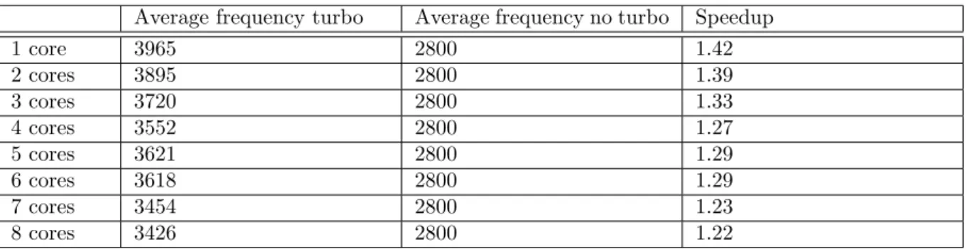
Average frequency turbo Average frequency no turbo Speedup

1 core 3965 2800 1.42 2 cores 3895 2800 1.39 3 cores 3720 2800 1.33 4 cores 3552 2800 1.27 5 cores 3621 2800 1.29 6 cores 3618 2800 1.29 7 cores 3454 2800 1.23 8 cores 3426 2800 1.22

Table 4.4: Average frequency on the 3 experiments and the expected speedup with respect to non-turbo frequency.

In Table 4.4, the average frequency can be seen across the three experiments, as well as the expected speedup calculated by dividing both frequencies as shown in Equation 4.2. When compared to Table 4.3, the relative speedup seems to grow accordingly. Note that the small difference could be explained explained by the CPI, that likely is not equal at different frequencies and different number of active cores.

This experiment concludes that Turbo Boost increases the performance of the processor, and the number of cores used affects the frequency at which the processor runs. The question that remains is about the cause that made the frequency drop when more cores were utilised when

(35)

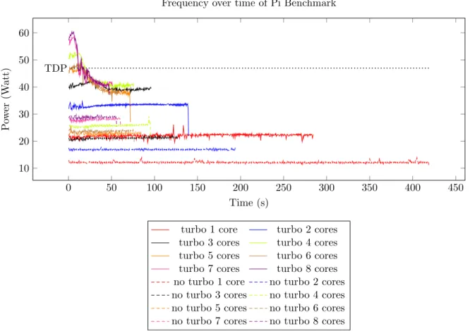
0 50 100 150 200 250 300 350 400 450 10 20 30 40 50 60 TDP Time (s) P ow er (W att)

Frequency over time of Pi Benchmark

Figure 4.3: The power over time of the first run of the Pi benchmark.

Turbo Boost was active. On Figure 4.3, the power consumption with the TDP are shown. As seen in Chapter 3, the processor should sustain a power at the PL1 which should be the TDP. But the power and thus also the frequency continued dipping below the TDP, which means that another factor was influencing power consumption. To explain this, in Figure 4.4, the temperature of the benchmark was plotted over time. An interesting observation can be made, as all the temperatures of the benchmark running on three or more cores are hitting the junction

temperature Tj, which for this processor is at 100◦C. As a consequence, the processor throttles

down its performance by reducing its frequency, which will reduce the power utilised and thus reduce its temperature.

In conclusion, there is a linear correlation between the frequency at which the processor is running and the obtained speedup. Even though Turbo Boost exceeds the sustainable power limit, it is limited by factors such as the temperature of the processor. This is not surprising, due to the fact that a MacBook computer is a compact machine, not allowing the processor to cool enough when the processor is under heavy load. This also shows that the processor in the MacBook computer, has more performance to offer, but cannot stretch its legs due to the cooling solution.

(36)

0 50 100 150 200 250 300 350 400 450 60 70 80 90 100 Time (s) T emp er ature ( ◦ C)

Temperature over time of the Pi benchmark

Figure 4.4: Temperature over time of the first run of the Pi benchmark.

4.3 Mixing-Compute Benchmark

In the first experiment, only a single benchmark was run to see what impact Turbo Boost would have. Now, it is clear that using Turbo Boost with a lot of cores could use up all the thermal headroom and power headroom. Therefore it would be interesting to see how the parallel part could impact the sequential part and by how much.

In this second experiment, multiple Pi-calculation benchmarks are chained one after another, by alternating a single-thread benchmark with a four-threaded one four times and ended with a single thread. Four threads are used to match the number of physical cores the MacBook machine has. Each run has to compute ten billion iterations in total. However, this time, the four-threaded version does not split the iterations evenly. The main thread has to run the ten billion iterations, while the other threads are also running the benchmark, but with the sole purpose of consuming resources. Once the main thread finishes the iterations, the other three threads are killed and the benchmark proceeds to the next single-threaded run, hence the similar compute time between the single- and four-threaded version.

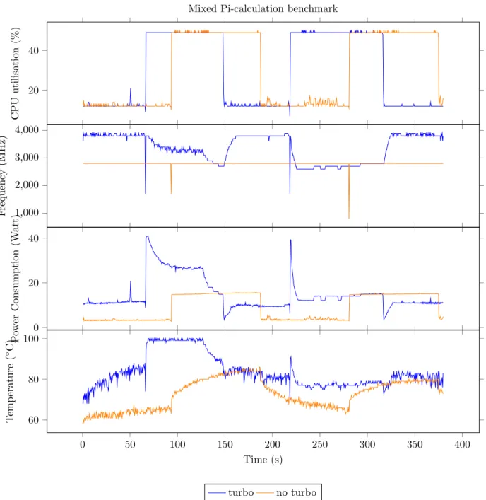
Figure 4.5 presents the results of the experiment. To keep the results clear, only the first two alternating iterations are shown, thus two times a single- followed by a four-threaded run.

The first observation is that the frequency during the single-threaded runs is always at turbo frequency when Turbo Boost is activated. This is expected, because the single-threaded run

(37)

20 40 CPU utilisation (% )

Mixed Pi-calculation benchmark

1,000 2,000 3,000 4,000 F requency (MHz) 0 20 40 P ow er Consumption (W att) 0 50 100 150 200 250 300 350 400 60 80 100 Time (s) T emp eratu re ( ◦C) turbo no turbo

Figure 4.5: Results of the mixed Pi-calculation benchmark, alternating between one and four threads. Only the first two pairs of single- and multi-threaded runs are shown.

does not use a lot of power when using Turbo Boost, around 11 Watt, which is below the TDP. This means that the single-threaded run could in theory keep running at the Turbo Boost frequency indefinitely. Another observation is that, when the four-threaded run finishes, it releases enough resources for the single-threaded run to regain the Turbo Boost frequency. Note that the frequency does not seem to jump directly to the Turbo boost frequency, but does this gradually.

However, power consumption always stays below the TDP, which means that there is still enough power headroom left to consume more power. This implies that the Turbo Boost