Dutch DisMod for several types of cancer | RIVM

Hele tekst

(1)research for man and environment. RIJKSINSTITUUT VOOR VOLKSGEZONDHEID EN MILIEU NATIONAL INSTITUTE OF PUBLIC HEALTH AND THE ENVIRONMENT. RIVM report 260751 004 Dutch DisMod for several types of cancer RT Hoogenveen, R Gijsen. September 2000. This investigation has been performed by order and for the account of Board of Directors of RIVM, within the framework of project 260751, Chronic Disease Modelling.. RIVM, P.O. Box 1, 3720 BA Bilthoven, telephone: 31 - 30 - 274 91 11; telefax: 31 - 30 - 274 29 71.

(2) Page 2 of 45. RIVM report 260751 004.

(3) RIVM report 260751 004. Page 3 of 45. Abstract Using a two-state Markov model we checked the consistency of incidence, prevalence and mortality data for specific types of cancer so as to construct an appropriate data set for chronic disease modelling. The data sources used were IKZ for regional cancer prevalence rates and survival proportions, NKR for national incidence rates, and CBS for national registered cause-specific mortality rates. Consistency checks were made for lung, rectal, colon, stomach, oesophagus, breast and prostate cancer. Using national incidence rates and regional survival proportions and a two-state transition model, we calculated prevalence and population mortality rates. We compared the calculated rates to empirical ones. For most types of cancer the calculated prevalence rates fitted well to the empirical ones, except for lung cancer (women), breast and prostate cancer. We found several possible explanations for these differences. The first one was double counts in case of multiple tumours. Based on data we corrected for double counts for breast cancer. The second explanation was differences between regional and national morbidity figures. These differences were clearly present for lung cancer and prostate cancer. The third explanation was past trends in disease incidence. Correcting for these trends resulted in smaller differences for all three cases. The calculated mortality rates fitted well to the empirical ones for the lethal types of cancer, but less well for those types of cancer with better prognosis, i.e. rectal and breast cancer. Next to double counts and past trends with respect to breast cancer these differences could be explained by excess mortality due to competing causes of death..


(5) RIVM report 260751 004. Page 5 of 45. Preface In the report 'Dutch DisMod. Constructing a set of consistent data for chronic disease modelling' (Hoogenveen et al., 2000) the results have been described of consistency checks on incidence, prevalence and mortality data for several chronic diseases including lung cancer. It was suggested that making the same type of analyses might be useful for several other types of cancer. We did not realise that the necessity of these analyses would become of current interest so soon after the publication of the report. New model calculations were needed to estimate the public health effects of different trends in food consumption on behalf of the Dutch Committee on Trends in Food Consumption. Therefore we needed good data on incidence and prognosis of several types of cancer. For lung cancer we already concluded that Dutch national incidence, and regional prevalence and survival data provided by NKR and IKZ respectively resulted in consistent model results for men. This makes a good starting point to do the same analyses for other types of cancer. We want to thank drs ME Kruijshaar for her comments on the draft version of this report, and ir AHP Luijben for his analyses on mortality data..


(7) RIVM report 260751 004. Contents Samenvatting 9 Summary 10 1.. Introduction 11. 2.. Data 12. 3.. Method 14. 4.. Lung cancer 16. 5.. Rectal cancer 19. 6.. Colon cancer 21. 7.. Stomach cancer 23. 8.. Cancer of oesophagus 25. 9.. Breast cancer 27. 10.. Prostate cancer 30. 11.. Discussion and conclusions 32. References 35 Appendix 1. Mathematical model equations 37. Appendix 2. Regional and national incidence rates 43. Appendix 3. Co-morbidity rates 44. Appendix 4. Mailing list 45. Page 7 of 45.


(9) RIVM report 260751 004. Page 9 of 45. Samenvatting Om te komen tot consistente verzamelingen van invoergegevens voor modellen van verschillende belangrijke vormen van kanker, hebben we de consistentie geanalyseerd van gegevens over incidentie, prevalentie en sterfte. Het gebruikte model betreft een zogenaamd Markov model met twee toestanden, waarin personen zich kunnen bevinden: met of zonder de ziekte. Dit model beschrijft de prevalentie en ziekte-specifieke sterfte van een cohort over de tijd als functie van de incidentie en ziekte-gerelateerde 'excess' sterfte. Regionale prevalentie- en overlevingsgegevens waren afkomstig van IKZ, landelijke incidentiegegevens van NKR, en landelijke geregistreerde sterftecijfers van CBS. We hebben de analyses uitgevoerd voor long-, endeldarm-, dikke darm, maag-, slokdarm-, borst- en prostaatkanker. Eerst zijn de gegeven relatieve overlevingspercentages omgezet in 'excess mortality rates'. Vervolgens is het model gebruikt om op basis van gegeven incidentie- en 'excess mortality' cijfers prevalentie- en sterftecijfers te berekenen. Deze zijn vergeleken met de empirische geregistreerde prevalentie- en oorzaak-specifieke sterftecijfers. De berekende en empirische prevalentiecijfers kwamen telkens goed overeen, behalve met name voor longkanker (vrouwen), borst- en prostaat-kanker. We hebben verschillende mogelijke verklaringen voor deze verschillen gevonden. De eerste mogelijke verklaring was dubbeltellingen in geval van multipele tumoren. Voor borstkanker waren hierover gegevens beschikbaar en is hiervoor gecorrigeerd. De tweede mogelijke verklaring was verschillen tussen regionale en landelijke ziektecijfers. Voor de drie genoemde gevallen waren de verschillen tussen de regionale en landelijke incidentiecijfers inderdaad in orde van grootte dezelfde als die tussen de empirische en (want gebaseerd op landelijke incidentiecijfers) berekende prevalentiecijfers. De derde mogelijke verklaring was trends over de tijd in de incidentie. Correctie hiervoor leidde inderdaad tot kleinere verschillen voor de genoemde kankervormen. Ook de berekende en empirische sterftecijfers kwamen telkens goed overeen. Uitzonderingen hierop waren de minder letale vormen van kanker, i.e. endeldarm- en borstkanker. Hier werd de empirische sterfte overschat. Naast de eerdergenoemde mogelijke verklaringen van dubbeltellingen en trends over de tijd voor borstkanker kunnen hier ook concurrerende doodsoorzaken een rol spelen. Deze mogelijke verklaring voor borstkanker en endeldarmkanker is ook in de literatuur gevonden. De conclusie luidt dat rekening houdend met dubbeltellingen in geval van multipele tumoren, verschillen tussen regionale en landelijke cijfers, trends over de tijd de incidentie- en relatieve overlevingscijfers van IKZ, prevalentiecijfers van NKR en sterftecijfers van CBS consistent zijn in de context van het 'two-state' transitiemodel. Er zijn aanwijzingen dat voor dikke darm, borst- en prostaatkanker concurrerende doodsoorzaken een rol spelen, maar literatuurgegevens hierover moeten nauwkeurig geïnterpreteerd worden..

(10) Page 10 of 45. RIVM report 260751 004. Summary A two-state transition model has been used to describe the disease-related mortality numbers and the change of disease prevalence numbers of a cohort over time using age-specific disease incidence rates, disease-related excess mortality rates, and mortality rates for other causes. Using this model we have checked the consistency of incidence, prevalence and mortality data for specific types of cancer so as to construct an appropriate data set for chronic disease modelling. Consistency checks have been made for lung, rectal, colon, stomach, oesophagus, breast and prostate cancer. We used cancer prevalence rates and relative survival proportions from one regional data source, and nationally registered incidence rates and cause-specific mortality rates. First, we transformed the relative survival proportions have been transformed to diseaserelated excess mortality rates. Then, the two-state transition model was used with age-specific incidence rates and disease-related excess mortality rates as input data to calculate prevalence and disease-specific mortality rates of the cohort over time. We compared the calculated prevalence and mortality rates to registered prevalence and mortality rates. For most types of cancer the calculated prevalence rates fitted well to the empirical ones, except for lung cancer (women), breast and prostate cancer. We have found several possible explanations for these differences. The first account was double counts of tumours. For breast cancer we had data on the proportion of newly diagnosed cases that already had a tumour in the other breast. The second account was differences between regional and national morbidity figures. For the three cases the differences between the regional and national incidence rates were approximately equal to the differences between the empirical regional prevalence rates and calculated (because based on empirical national incidence rates) national prevalence rates. The third explanation was past trends in disease incidence. As a result of increasing incidence rates, prevalence rates calculated from current incidence rates overestimate current prevalence rates. Correcting for reported past trends in disease incidence resulted in smaller differences for lung cancer (women), breast and prostate cancer. For most types of cancer also the calculated disease-specific mortality rates fitted well to the registered cause-specific mortality rates. For the less lethal types of cancer, i.e. rectal and breast cancer, the calculated mortality overestimated the registered one. Apart from the double counts and time trends in case of breast cancer another explanation was found, excess mortality due to competing death risks. This explanation has also been reported in the literature..

(11) RIVM report 260751 004. 1.. Page 11 of 45. Introduction. In the report 'Dutch DisMod. Constructing a set of consistent data for chronic disease modelling' (Hoogenveen et al., 2000) the results have been described of consistency checks on several chronic diseases, including lung cancer. The consistency of disease incidence, prevalence and mortality data was checked within the chronic diseases model context. The method of consistency checking has been described in chapter 3. In this study we applied the same method to several other types of cancer, including cancer of the lung, rectum, colon, stomach, oesophagus, breast, and prostate. The resulting internally consistent incidence, prevalence and mortality rates will be used for new applications of the chronic diseases model. In the first place we will use them to calculate trends in incidence and mortality rates for several types of cancer from different scenarios on trends in the consumption of fruit and vegetables, saturated fat and trans fatty acids on behalf of the Committee on Trends in Food Consumption of the Dutch Health Council. Other model applications will follow. In chapter 2 we describe the data we used in the calculations. In chapter 3 the method of consistency checks is explained. Special attention is given to aspects that have to be taken into account when making the consistency checks, i.e. regional versus national morbidity figures, time trends, and multiple tumours. In the chapters 4-10 the results of the consistency checks for each of the different types of cancer are described. In each chapter the specific data assumptions, the results of the consistency checks and a discussion of these results are presented. First, we start with the simple consistency checks, i.e. with regional prevalence and survival data and national incidence data, without adjustment for time trends or multiple tumours (except for breast cancer). For lung cancer (women), breast and prostate cancer we made additional calculations including adjustment for time trends. In chapter 11 the results are discussed in general and some conclusions are drawn. The model and some data are described in more detail in separate appendices. In Appendix 1 the mathematical model equations are described. In Appendix 2 the differences between the regional and national incidence figures are presented. In Appendix 3 the cancer and cardiovascular diseases prevalence rates among the newly diagnosed cancer patients have been compared to the population rate values..

(12) Page 12 of 45. 2.. RIVM report 260751 004. Data. The data sources that have been used were similar to the ones that we used for the previous consistency checks (Hoogenveen et al., 2000). Table 1: Data sources used Source. Data. Netherlands Cancer Registry (NKR) Eindhoven Cancer Registry. disease incidence rates disease prevalence rates and relative survival proportions cause-specific population mortality rates trends in disease incidence, prevalence and cause-specific mortality rates, and general background information background information on co-morbidity and mortality. Statistics Netherlands (CBS) VTV-document (Maas et al., 1997). literature. The Eindhoven Cancer Registry started in 1955 as part of a programme for nationwide cancer registration in the area of south-eastern part of the region North Brabant. In 1970 the registry covered a population of about 1 million inhabitants. Within the framework of the Comprehensive Cancer Centre South (IKZ) more than 2 million people have been covered since 1988. The nine regional Comprehensive Cancer Centres have formed the national Association of Comprehensive Cancer Centres in 1989, the Netherlands Cancer Registry (NKR), that started in 1989. Since then national incidence numbers have been available on a yearly basis. Survival rates have been calculated from the follow-up of past newly diagnosed cases. Because the national registry started just in 1989 only regional survival data have been available. Regional cancer prevalence numbers have been calculated by combining the information from past incidence numbers and follow-up data. Since the assessment of the prevalence numbers is a very time-consuming process, they have been presented for some years only so far. Statistics Netherlands (CBS) provides national mortality numbers, i.e. the number of deceased persons with the cancer type registered as the primary cause of death. We have used 1994 incidence, 1993 prevalence and 1994 cause-specific mortality rates, specified by gender and 5-year age-classes. The survival data used were from period 19881992. In case of clear trends in survival we have extrapolated the survival data to values for year 1994. The survival figures used were specified by three age-classes: <60, 60-74, and ≥75.

(13) RIVM report 260751 004. Page 13 of 45. years. We have made analyses for several cancer of the lung (ICD 162), rectum (ICD 154), colon (ICD 153), stomach (ICD 151), oesophagus (ICD 150), breast (ICD 174-175), and prostate (ICD 185). We did not distinguish between different stages of these cancers. As a consequence, when we use the term 'cancers of the same type', we use the characterisation by ICD-code given above..

(14) Page 14 of 45. 3.. RIVM report 260751 004. Method. Introduction We have shown that an important problem in chronic disease modelling is the lack of good data on the survival of persons with chronic diseases in the general population (Hoogenveen et al., 2000). We estimated the excess mortality rates for these persons from data on disease incidence and prevalence, using a two-state transition model. To validate these mortality rates, we compared the calculated mortality rate ratios and disease duration times to figures from literature. For lung cancer we concluded that regional survival and prevalence data and national incidence data fitted well together for men. Based on this conclusion we used in this study survival data to calculate prevalence rates to make the consistency checks, instead of using prevalence data to calculate survival rates (see also chapter 11 'Discussion'). Chronic diseases model The model we used is a two-state transition model (see Appendix 2). The model describes the change of total population and disease prevalence numbers for a birth cohort for one disease. Disease-specific incidence and excess mortality rates were the model input. Disease-specific prevalence and population mortality rates were the model output. We compared the calculated disease prevalence rates to empirical values, and the calculated mortality rates to the registered cause-specific rates. Mortality is defined proportional to the disease prevalence in the model. Thus, the 1-year survival rates used in the model are the average of the 1-year survival rates for all patients. However, the survival data refer to newly diagnosed cases. As 1-year survival rates generally increase for increasing past disease time period, the 1-year survival rates for prevalent cases are generally higher than those for newly diagnosed cases. We have therefore assumed that the 1-year survival rates used in the model can be approximated by the fifth power root of the 5-year survival rates. The absolute 5-year survival rates have been calculated using the relative 5-year survival proportions provided by IKZ and the 1994 Dutch total mortality rates (Appendix 1). Time trends The model equations have been derived assuming time-constant disease incidence and survival rates. In other words, we have assumed a steady-state situation. As a result, the calculated prevalence figures for a birth-cohort coincide with those for the current population. For several types of cancer, past trends in disease incidence have been reported, and so the steady-state assumption was violated. As a result, prevalence rates calculated from current incidence rates overestimate current prevalence rates in case of increasing incidence rates over time. To correct for past trends, we have calculated for each age-year (cohort) separately the current prevalence rate from past incidence rates explicitly taking account of the change in.

(15) RIVM report 260751 004. Page 15 of 45. the disease incidence over time (see Appendix 1). We assumed that the yearly relative change of the age-specific incidence rates over time was the same for all ages. Differences between regional and national figures We have used national cancer-specific incidence rates, but regional prevalence rates and survival proportions. For some types of cancer the regional incidence rates were clearly different from the national ones (see Appendix 2). One important explanation is different smoking rates. We had no data to compare regional and national survival. We did not expect large differences between regional and national survival rates, for example because of standard cancer treatment procedures and, for breast cancer, standard national screening protocols. However, screening for breast cancer started later in the Southeast than in the rest of the Netherlands. Assuming identical survival rates and time-constant parameters, we expect the differences between the calculated and empirical prevalence rates to be in the same direction and magnitude as the differences between the national and regional incidence rates. Multiple tumours The incidence rates provided by NKR refer to newly diagnosed tumours, and not to new patients. To deal with this problem we have to distinguish between cancers of the same type and those of different types (using the characterisation by ICD-code), and between prevalence and mortality. When the secondly diagnosed tumour is of the same type as the first one, the person is counted twice, and both disease prevalence and mortality numbers are overestimated. We have corrected for double counts for breast cancer. When the secondly diagnosed cancer is of another type than the first one, the person is counted as a case for both types of cancer. In case of disease prevalence this is not problematic, since prevalence has been defined as having at least the specific disease. However, co-morbidity may complicate the interpretation of the model results and data with respect to mortality (see also Appendix 3). Persons having a type of cancer may have an increased risk for other chronic diseases, for example another type of cancer, compared to those without this cancer. Moreover, this other chronic disease might be more lethal. As a result, part of the excess mortality of specific cancer types might be caused by this other disease, or stated otherwise, might be coded with this disease as the primary cause of death. This phenomenon is called 'dependent competing death risks'..

(16) Page 16 of 45. 4.. RIVM report 260751 004. Lung cancer. Since prognosis of lung cancer has not changed much during the last decades, we have used the 1988-1992 relative 5-year survival proportions: 18% (age<60), 13% (age 60-74) and 5.7% (age≥75) (Coebergh et al., 1995). Given lung cancer incidence rates and relative survival proportions, we calculated prevalence and population mortality rates, and compared them to empirical rate values (Figure 1 for men, Figure 2 for women). incidence. rates. rate 0.007 0.006 0.005 0.004 0.003 0.002 0.001 20. 40. 60. prevalence rate 0.0175 0.015 0.0125 0.01 0.0075 0.005 0.0025. 80. age Hyears L. rates. calculated registered. 20. 40. mortality. 60. 80. age H years L. rates. rate calculated. 0.008. registered. 0.006 0.004 0.002 20. 40. 60. 80. age Hyears L. Figure 1: incidence, prevalence and mortality rates for lung cancer for men.

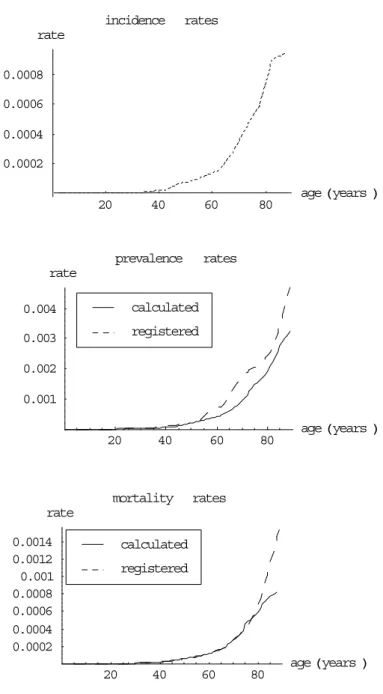
(17) RIVM report 260751 004. Page 17 of 45. incidence. rates. rate 0.0008 0.0006 0.0004 0.0002 20. 40. 60. prevalence. age Hyears L. 80. rates. rate 0.002 calculated 0.0015. registered. 0.001 0.0005 20. 40. mortality. 60. 80. age Hyears L. rates. rate 0.0008. calculated. 0.0006. registered. 0.0004 0.0002 20. 40. 60. 80. age H years L. Figure 2: incidence, prevalence and mortality rates for lung cancer for women The figures show that the calculated lung cancer prevalence and mortality rates fitted well to the empirical ones, except for elderly persons and the prevalence rates for women. The smaller calculated prevalence rates for men compared to the empirical ones for elderly men can be explained by the smaller national incidence rates compared to the regional ones (Appendix 2). The sharp change of the curve at age 75 results from the change of relative survival proportion from 13% to 5.7%. The large differences between empirical and calculated prevalence rates for men can be explained mainly by the regional incidence rates being smaller than the national ones (Appendix 2). This difference also explains why the calculated mortality rates are almost equal to the nationally registered cause-specific mortality rates. Moreover, incidence rates have increased for Dutch women as a result of increasing.

(18) Page 18 of 45. RIVM report 260751 004. smoking rates in the past, especially for age 60-75 years between 1968 and 1992. Consequently, the calculated prevalence rates overestimated the empirical rates. Following Coebergh et al. (1995) we assumed that incidence rates have increased with yearly 5% over the past and that survival rates were constant. The calculated lung cancer prevalence rates adjusted for this trend are presented in Figure 3.. prevalence rate 0.002. rates. unadjusted adjusted empirical. 0.0015 0.001 0.0005 20. 40. 60. 80. age Hyears L. Figure 3: calculated prevalence rates for lung cancer for women adjusted for incidence time trends The adjustment for incidence time trends resulted in only slightly better fits. This is not very surprising, since the disease duration of lung cancer is relatively small..

(19) RIVM report 260751 004. 5.. Page 19 of 45. Rectal cancer. The relative 5-year survival proportions were almost independent of age, and have increased almost linearly since 1955 (Coebergh et al., 1995). We extrapolated the time trend for survival resulting in an approximate value of 60% for both men and women for year 1994. Given rectal cancer incidence rates and relative survival proportions, we calculated prevalence and mortality rates, and compared them to empirical rate values (Figure 4 for men, Figure 5 for women). incidence. rates. rate 0.00175 0.0015 0.00125 0.001 0.00075 0.0005 0.00025 20. 40. 60. prevalence. 80. age Hyears L. rates. rate 0.02 calculated 0.015. registered. 0.01 0.005. 20. 40. 60. mortality. rates. 80. age Hyears L. rate 0.0012 calculated. 0.001. registered. 0.0008 0.0006 0.0004 0.0002 20. 40. 60. 80. age Hyears L. Figure 4: incidence, prevalence and population mortality rates for rectal cancer for men.

(20) Page 20 of 45. RIVM report 260751 004. incidence. rates. rate 0.0008 0.0006 0.0004 0.0002 20. 40. 60. prevalence. 80. age Hyears L. rates. rate 0.008 calculated 0.006. registered. 0.004 0.002. 20. 40. 60. mortality. rates. 80. age Hyears L. rate 0.0006 0.0005 0.0004 0.0003 0.0002. calculated registered. 0.0001 20. 40. 60. 80. age Hyears L. Figure 5: incidence, prevalence and population mortality rates for rectal cancer for women The calculated rectal cancer prevalence rates fitted very well to the empirical rate values. The regional incidence rates are indeed similar to the national ones. However, the mortality rates were overestimated. This could be the result of excess mortality to other causes. This conjecture was confirmed by several studies that showed that patients with rectal cancer have a great risk of having other types of cancer (Manton et al., 1991; Wagner et al., 1993; Coebergh et al., 1995; Garcia-Anguiano et al., 1995; Payne&Meyer, 1995)..

(21) RIVM report 260751 004. 6.. Page 21 of 45. Colon cancer. The characteristics of colon cancer are similar to those of rectal cancer. The Dutch relative 5year survival proportions have also increased almost linearly during the last decades from 49% in 1955-1969 to 57% in 1987-1992, and were almost independent on age. We again extrapolated the time trend in survival resulting in an approximate value of 60% for both men and women. Given colon cancer incidence rates and relative survival proportions, we calculated prevalence and mortality rates, and compared them to empirical rate values (Figure 6 for men, Figure 7 for women). incidence. rates. rate 0.0025 0.002 0.0015 0.001 0.0005 20. 40. prevalence. 60. 80. age Hyears L. rates. rate 0.025. calculated. 0.02. registered. 0.015 0.01 0.005 20. 40 mortality. 60 rates. 80. 60. 80. age Hyears L. rate 0.0035 0.003 0.0025 0.002 0.0015 0.001 0.0005. calculated registered. 20. 40. age Hyears L. Figure 6: incidence, prevalence and population mortality rates for colon cancer for men.

(22) Page 22 of 45. RIVM report 260751 004. incidence. rates. rate 0.0025 0.002 0.0015 0.001 0.0005 20. 40. prevalence. 60. 80. age Hyears L. rates. rate 0.02. calculated. 0.015. registered. 0.01 0.005 20. 40. 60. mortality. 80. age Hyears L. rates. rate 0.003 calculated. 0.0025. registered. 0.002 0.0015 0.001 0.0005 20. 40. 60. 80. age Hyears L. Figure 7: incidence, prevalence and population mortality rates for colon cancer for women Both the calculated prevalence and (contrary to rectal cancer) mortality rates fitted well to the empirical data, except for elderly people. This difference between rectal and colon cancer is remarkable, since the prognoses are almost identical. This difference was reported by Percy et al. (1981), who found an over-reporting of colon cancer mortality and under-reporting of rectal cancer mortality..

(23) RIVM report 260751 004. 7.. Page 23 of 45. Stomach cancer. Dutch stomach cancer incidence rates have decreased from 1992-1995. The registered population mortality rates have decreased for a longer period. The prevalence rates have increased with 10% between 1990 and 1993. Regional relative survival proportions showed an improvement around 1980, but only for ages below 70 years. In absolute numbers, the prognosis of stomach cancer patients is still bad. Following IKZ data the relative 5-year survival proportion is 25% for ages below 75 years, and 20% for higher ages. Given stomach cancer incidence rates and relative survival proportions, we calculated prevalence and mortality rates, and compared them to empirical rate values (Figure 8 for men, Figure 9 for women). incidence. rates. rate 0.002 0.0015 0.001 0.0005 20. 40. prevalence. 60. 80. age Hyears L. rates. rate 0.008. calculated. 0.006. registered. 0.004 0.002 20. 40. mortality. 60. 80. age Hyears L. rates. rate 0.0025. calculated. 0.002. registered. 0.0015 0.001 0.0005 20. 40. 60. 80. age Hyears L. Figure 8: incidence, prevalence and population mortality rates for stomach cancer for men.

(24) Page 24 of 45. RIVM report 260751 004. incidence. rates. rate 0.0008 0.0006 0.0004 0.0002 20. 40. 60. prevalence. 80. age Hyears L. rates. rate 0.004. calculated. 0.003. registered. 0.002 0.001 20. 40. 60. mortality. rates. 80. age Hyears L. rate 0.0014 0.0012 0.001 0.0008 0.0006 0.0004 0.0002. calculated registered. 20. 40. 60. 80. age Hyears L. Figure 9: incidence, prevalence and population mortality rates for stomach cancer for women The calculated stomach cancer prevalence and population mortality rates fitted well to the empirical rate values, except for the prevalence rates for women. The latter difference can be explained by the difference between regional and national incidence rates (Appendix 2). The good fit on mortality relates to the high lethality of stomach cancer..

(25) RIVM report 260751 004. 8.. Page 25 of 45. Cancer of oesophagus. Incidence and mortality rates of oesophagal cancer have increased with approximately 5% yearly in the Netherlands. The prognosis of cancer of oesophagus is bad compared to most other types of cancer. As a result we used 1-year instead of 5-year relative survival proportions to describe the excess mortality. Following (Coebergh et al., 1995) the relative survival proportion is 35%. Given incidence rates and relative survival proportions, we calculated prevalence and mortality rates, and compared them to empirical rate values. incidence. rates. rate 0.0005 0.0004 0.0003 0.0002 0.0001 20. 40. prevalence. 60. 80. age Hyears L. rates. rate 0.0007 0.0006 0.0005 0.0004 0.0003 0.0002 0.0001. calculated registered. 20. 40. mortality. 60. 80. age Hyears L. rates. rate 0.001. calculated. 0.0008. registered. 0.0006 0.0004 0.0002 20. 40. 60. 80. age Hyears L. Figure 10: incidence, prevalence and population mortality rates for cancer of oesophagus for men.

(26) Page 26 of 45. RIVM report 260751 004. incidence. rates. rate 0.0003 0.00025 0.0002 0.00015 0.0001 0.00005 20. 40. 60. prevalence. 80. age Hyears L. rates. rate 0.0003 0.00025 0.0002 0.00015 0.0001 0.00005. calculated registered. 20. 40. mortality. 60. 80. age Hyears L. rates. rate 0.0004 calculated 0.0003. registered. 0.0002 0.0001 20. 40. 60. 80. age Hyears L. Figure 11: incidence, prevalence and population mortality rates for cancer of oesophagus for women The prevalence rates were slightly overestimated for men. The main explanation we found was that the regional incidence rates were smaller than the national ones resulting in empirical prevalence rates that were smaller than the calculated ones (Appendix 2). The calculated mortality rates fitted well to the data. Due to the bad prognosis of cancer of oesophagus the effect of excess mortality from competing causes of death is probably small..

(27) RIVM report 260751 004. 9.. Page 27 of 45. Breast cancer. Since breast cancer incidence rates are very small for men, we only considered breast cancer for women. Dutch breast cancer incidence rates have steadily increased in the past years with approximately yearly 1% for all ages until 1990 and 3% afterwards (Coebergh et al., 1995; Voogd et al., 1997). The relative survival proportions have increased during 70's and 80's, but since then the increase has stopped (Coebergh et al., 1995). The relative survival proportions were almost equal for all ages. We have assumed that 8% of all new breast cancer cases refer to persons already having had a tumour in the other breast (Voogd et al., 1997). Following Coebergh et al. (1995) the 5-year relative survival proportion used is 76%. Given incidence rates and survival proportions, we calculated prevalence and mortality rates and compared them to empirical rate values (Figure 12). incidence. rates. rate. 0.003 0.002 0.001. 20. 40. 60. prevalence. 80. age H years L. rates. rate 0.05. calculated. 0.04. registered. 0.03 0.02 0.01 20. 40 mortality. 60. 80. age Hyears L. rates. rate 0.0035 0.003 0.0025 0.002 0.0015 0.001 0.0005. calculated registered. 20. 40. 60. 80. age H years L. Figure 12: incidence, prevalence and population mortality rates for breast cancer for women Note: incidence includes 8% second tumours, calculated prevalence and mortality adjusted for second tumours.

(28) Page 28 of 45. RIVM report 260751 004. The calculated breast cancer prevalence and mortality rates are larger than the empirical ones. One possible explanation for the overestimation of the prevalence rates is the difference between regional and national incidence rates for middle ages (Appendix 2). Another explanation for the overestimation of both prevalence and mortality rates is the increase of the incidence rates over the past. As we already have explained in chapter 3 ('Method') the result of this trend is that the calculated prevalence and mortality rates based on current incidence rates overestimate current empirical rates. We have calculated new prevalence rates by adjusting the past national incidence rates for the time trend, assuming that the time trend was equal for all ages. According to Coebergh et al. (1995) we have assumed constant survival rates.. Figure 13: calculated prevalence rates for breast cancer for women adjusted for incidence time trends The newly calculated prevalence rates adjusted for incidence time fitted better to the empirical ones. The relative difference between the calculated and empirical prevalence rates is of the same magnitude as the relative difference between national and regional incidence rates (Appendix 2). Another possible explanation for the differences between the calculated. prevalence. rates. rate unadjusted adjusted empirical. 0.05 0.04 0.03 0.02 0.01 20. 40. 60. 80. age Hyears L. and empirical mortality rates is again excess mortality due to competing causes of death, although one has to take into account mortality due to other causes. It has been shown that patients with breast cancer have an increased risk of already having other types of cancer (Coebergh et al., 1995; Appendix 3). Brown et al. (1993) reported that breast cancer patients have an overall non-cancer relative mortality risk of 1.09 compared to women without breast cancer. Several studies reported on the proportion of breast cancer patients that die with breast cancer registered as the primary cause of death. For approximately 89% of Dutch mortality cases with breast cancer registered on the death certificate, it was the primary cause of death (Statistics Netherlands, 2000). Mueller and Jeffries (1975) concluded that 80-85% of all women who die after developing breast cancer die of their breast cancer. Fish et al. (1998) found in a follow-up study that almost 90% of women with breast cancer die from breast.

(29) RIVM report 260751 004. Page 29 of 45. cancer. However, these figures do not differ much from the proportions that one would expect (Appendix 1): 95% until age 60, 90% until age 70, and 81% until age 80 years. Next to the possible explanations given above also incompleteness of prevalence might also be en explanatory factor for the higher estimates. The registered prevalence numbers are based on past incidence registrations, and in the early years the cancer registry was less complete than in later years (Schouten et al., 1993)..

(30) Page 30 of 45. 10.. RIVM report 260751 004. Prostate cancer. Coebergh et al. (1995) have presented age-specific 5-year relative survival proportions for 1980-1992. The general conclusion from these trends is that for younger ages survival has hardly improved, but for higher ages an improvement of survival since 1980 has been found. We have assume that the 5-year relative survival proportions are 58% (age<60), 64% (60-74), and 58% (>75). Given prostate cancer incidence rates and relative survival proportion, we have calculated prevalence and mortality rates, and compared them to empirical rate values (Figure 14).. incidence. rates. rate 0.008 0.006 0.004 0.002 20. 40. prevalence. 60. 80. age Hyears L. rates. rate 0.08 calculated 0.06. registered. 0.04 0.02. 20. 40. mortality. 60. 80. age Hyears L. rates. rate 0.012. calculated. 0.01. registered. 0.008 0.006 0.004 0.002 20. 40. 60. 80. age Hyears L. Figure 14: incidence, prevalence and population mortality rates for prostate cancer.

(31) RIVM report 260751 004. Page 31 of 45. The calculated prevalence rates were larger than the empirical ones. The differences between regional and national incidence rates seem to be small, when we take account of the differences in measurement time points (Appendix 2). A more important explanation is that incidence rates have increased in the past, resulting in current prevalence rates being 'too small' compared to current incidence rates. Following Coebergh et al. (1995) we have assumed that incidence rates have increased with yearly 5% over the past and that survival rates were constant. We have calculated new prevalence rates by adjusting the past national incidence rates for the time trend, assuming that the time trend was equal for all ages (Figure 15).. prevalence rate 0.08. rates. unadjusted adjusted empirical. 0.06 0.04 0.02. 20. 40. 60. 80. age Hyears L. Figure 15: calculated prevalence rates for prostate cancer for men adjusted for incidence time trends The calculated prevalence rates adjusted for past incidence time trends were indeed smaller. After adjustment for incidence time trends, the calculated mortality is of the same magnitude as the empirical mortality, although we expected a small overestimation according to literature. Brown et al. (1993) reported that prostate cancer patients have an overall noncancer relative mortality risk of 1.14 compared to men without prostate cancer. Coebergh et al. (1995) have shown that newly diagnosed prostate cancer cases have high risks of having also cardiovascular diseases. Satariano et al. (1998) found that 54% of 584 deceased prostate carcinoma patients died of their prostate carcinoma. Newschaffer et al. (2000) even found a percentage of only 39%. These percentages are lower than the expected ones (see Appendix 1): 93% until age 60, 81% until age 70 and 67% until age 80..

(32) Page 32 of 45. 11.. RIVM report 260751 004. Discussion and conclusions. The regional relative 5-year survival proportions combined with national incidence rates resulted in calculated prevalence rates that generally fitted well to empirical regional prevalence rates. The differences were especially small for cancer of the lung (men), rectum, colon, stomach, and oesophagus. Relatively large differences were found for lung cancer (women), rectal cancer (mortality), breast cancer and prostate cancer. These differences could be explained by multiple tumours (breast cancer), time trends in incidence (lung cancer, breast cancer and prostate cancer), or with respect to the prevalence by differences between regional and national incidence rates (lung cancer, breast cancer and prostate cancer). For mortality the model fits were often also good, except for lung cancer (women), rectal, breast and prostate cancer. Next to the first two explanations given above, mortality differences could also be explained by excess mortality due to competing causes of death. The possible explanation of competing causes of death was confirmed by literature, although one has to take account of the mortality due to other causes in case of cancers that are not highly lethal. We comment on these explanations in more detail below. Multiple tumours Correction for multiple tumours of the same type is easy by subtracting the proportion of tumours that are not the first one from the incidence rates. For breast cancer it was shown that 7-9% of the newly diagnosed cases had another tumour in the other breast. For other types of cancer with possibly multiple tumours of the same type (colorectal cancer) we had no data. When the secondly diagnosed type of cancer is different from the first one (following our ICD-based characterisation), it has no effect on the prevalence rates. The reason is that the disease prevalence rates describe the population fractions with the specific cancer type but maybe also other types of cancer. The effect on the mortality rates is probably larger (see 'Competing causes of death') Differences between regional and national figures Cancer incidence rates were available on both regional and national level, prevalence rates and relative survival proportions only on regional level. For some types of cancer clear differences between regional and national incidence rates have been found: lung cancer (women), stomach cancer (women), oesophagal cancer, and breast cancer for middle ages. One important possible explanation is different smoking patterns. For all types of cancer where regional and national incidence rates clearly were different, the differences between the empirical regional and calculated national (because based on national incidence rates) prevalence rates were similar..

(33) RIVM report 260751 004. Page 33 of 45. Time trends Time trends in disease incidence and/or survival rates result in time trends in disease prevalence, however with different rates of change (see Appendix 2). The effect of time trends has clearly been shown for lung cancer (women), breast and prostate cancer. Adjusting for incidence time trends highly improved the fit of the calculated prevalence rates. Competing causes of death Registered cause-specific mortality statistics describe the numbers of deceased persons specified by the primary cause of death. IKZ cancer-specific survival rates describe the prognosis of newly diagnosed patients. Even though for these patients the cancer type is the most likely cause of future death, they are exposed to all other causes of death during their disease period. For rectal cancer and breast cancer the calculated excess mortality rates are higher than the registered cause-specific ones, which may point at excess mortality from competing causes of death. Empirical information on competing causes of death can be found from data on co-morbidity and from registered primary and secondary cause of death mortality numbers. Although the prognoses for rectal and colon cancer do not differ much, our results suggest that colon cancer is more often reported as cause of death than rectal cancer, as was confirmed by literature. When interpreting the number of deceased people with a specific disease registered as the primary or secondary cause of death, one has to take account of the background mortality due to other causes. Highest ages For the highest ages there is the twofold problem of data and model inaccuracies. The data showed large variations due to small numbers. Moreover, determining the cause of death can be difficult for these ages. The model results for the highest ages were not very reliable, since we used extrapolation to get year-specific numbers for ages above 80 years instead of interpolation for lower ages. Numerical errors The incidence-prevalence-mortality (IPM) model describes the relation between age-specific disease incidence, prevalence and mortality rates. Given two of the three variables, the other one can be calculated. In the first analyses (Hoogenveen et al., 2000) excess mortality rates were calculated from given disease incidence and prevalence rates. In the analyses that have been described in the current report prevalence rates have been calculated from given disease incidence and excess mortality rates. The former model application is numerically much less stable than the latter one. The reason is that mortality rates have to be calculated from differences between prevalence rates for successive age-years. Therefore, in terms of error propagation and model sensitivity, calculating prevalence rates is highly favourable to calculating incidence or mortality rates, using the IPM-model structure..

(34) Page 34 of 45. RIVM report 260751 004. Disease duration We assumed in the model that the mortality was independent on disease duration. However, the empirical relative survival proportions from IKZ and other studies have shown that for many types of cancer the prognosis improves with disease duration time. That means, the 1year survival rates are lower for newly diagnosed cases than for cancer patients that have survived a given time period. The consistency analyses have been made to construct an appropriate data set for chronic disease modelling. These models are used to describe the public health effects of trends in or interventions on disease risk factors in the context of multiple risk factors and diseases. For this aim the assumption of duration-independent mortality is valid. If one wants to distinguish different disease stages so as to describe (for example) the effects of stage-specific trends or interventions, the assumption is too crude. Our final conclusion is that for the types of cancer selected the incidence data from NKR and prevalence and survival data from IKZ fit well together when taking account of differences between regional and national figures, time trends and multiple tumours. For the less lethal types of cancer, i.e. rectal, breast and prostate cancer, we found differences between diseaserelated excess mortality and registered cause-specific mortality. When combining the different types of cancer in one model one has to take explicitly account of this difference..

(35) RIVM report 260751 004. Page 35 of 45. References Barendregt JJ, van Oortmarssen GJ, Hout BA van, Bosch JM van den, Bonneux L. Coping with multiple morbidity in a life table. Mathematical Population Studies (1998), vol 7: 1, pp 29-49 Berrino F, Sant M, Verdecchia A, Capocaccia R, Hakulinen T, Estève J (eds.) Survival of cancer patients in Europe. The EUROCARE Study. IARC Scientific Publications no. 132, Lyon, 1995 Brown BW, Brauner C, Minnotte MC. Noncancer deaths in white adult cancer patients. Journal of the National Cancer Institute (1993), vol 85: 12, pp 979-987 Coebergh JWW, Heijden LH van der, Janssen-Heijnen MLG (eds.) Cancer incidence and survival in the Southeast of the Netherlands 1955-1994. Integraal Kankercentrum Zuid, Eindhoven, 1995 Coebergh JW, Janssen-Heijnen ML, Post PN, Razenberg PP. Serious co-morbidity among unselected cancer patients newly diagnosed in the southeastern part of The Netherlands in 1993-1996. Journal of Clinical Epidemiology (1999), vol 52: 12, pp 1131-1136 Fish EB, Chapman JA, Link MA. Competing causes of death for primary breast cancer. Annals of Surgical Oncology (1998) vol 5: 4, pp 368-375 Garcia-Angioano F, Marchena Gomez J, Morales JA, Gomez Guerra G, Conde Martel A, Cruz Benavides F. Colorectal cancer in the context of multiple primary malignant neoplasms. Revista Espanola de Enfermedades Digestivas (1995), vol 87: 5, pp 369-374 Grulich AE, Swerdlow AJ, dos Santos Silva I, Beral V. Is the apparent rise in cancer mortality in the elderly real? Analysis of changes in certification an coding of cause of death in England and Wales, 1970-1990. International Journal of Cancer (1995), vol 63: 2, pp 164-168 Heinävaara S, Hakulinen T. Relative survival of patients with multiple cancers. In: Proceedings of the XXth International Biometric Conference, July 1-7, 2000, University of California at Berkely Hoogenveen RT, Gijsen R, Genugten MLL van, Kommer GJ, Schouten JSAG, Hollander AEM de. Dutch DisMod. Constructing a set of consistent data for chronic disease modelling. RIVM report 260751 001. RIVM, Bilthoven, 2000 Kruijshaar ME, JJM Barendregt, Hoeymans N. The use of models in estimating disease epidemiology. (2000) Submitted Maas IAM, Gijsen R, Lobbezoo IE, Poos MJJC. Public Health Status and Forecasts 1997. I. The public health status: an update. Maas IAM, Gijsen R, Lobbezoo IE, Poos MJJC (eds.). RIVM, Bilthoven; Elsevier/De Tijdstroom, Maarssen, 1997 (in Dutch) Mannino DM, Ford E, Giovino GA, Thun M. Lung cancer deaths in the United States from 1979 to 1992: an analysis using multiple-cause mortality data. International Journal of Epidemiology (1998), vol 27: 2, pp 159166 Manton KG, Wrigley JM, Cohen HJ, Woodbury MA. Cancer mortality, aging, and patterns of co-morbidity in the United States: 1968 to 1986. Journal of Gerontology (1991), vol 46: 4, pp S225-234 Mueller CB, Jeffries W. Cancer of the breast: Its outcome as measured by the rate of dying and causes of death. Annals of Surgery (1975), vol 182: 3, pp 334-341 Murray CJL, Lopez AD (eds.). Global Burden of Disease -- A comprehensive assessment of mortality and disability from diseases, injuries, and risk factors in 1990 and projected to 2020. Volume I. WHO, Geneva, 1996.

(36) Page 36 of 45. RIVM report 260751 004. Newschaffer CJ, Bush TL, Penberthy LE, Bellantoni M, Helzlsour K, Diener-West M. Does comorbid disease interact with cancer? An epidemiologic analysis of mortality in a cohort of elderly breast cancer patients. Journals of Gerontology. Series A, Biological Sciences and Medical Sciences (1998), vol 53: 5, pp M372-378 Newschaffer CJ, Otani K, McDonald MK, Penberthy LT. Causes of death in elderly prostate cancer patients and in a comparison nonprostate cancer cohort. Journal of the National Cancer Institute (2000), vol 92: 8, pp 613621 Payne JE, Meyer HJ. The influence of other diseases upon the outcome of colorectal cancer patients. Australian and New Zealand Journal of Surgery (1995), vol 65: 6, pp 398-402 Percy C, Stanek E 3d, Gloeckler L. Accuracy of acncer death certificates and its effect on cancer mortality statistics. American Journal of Public Health (1981), vol 71: 3, pp 242-250 Reynolds DL, Nguyen VC, Clarke EA. Reliability of cancer mortality statistics in Ontario: a comparison of incident and death diagnoses, 1979-1983. Canadian Journal of Public Health (1991), vol 82: 2, pp 120-126 Roberts MG, Tobias MI. The use of multi-state life-tables for improving population health. (2000) Submitted Satariano WA, Ragland KE, Eeden SK van den. Cause of death in men diagnosed with prostate carcinoma. Cancer (1998), vol 83: 6, pp 1180-1188 Schouten LJ, Hoppener P, Brandt PA van den, Knottnerus JA, Jager JJ. Completeness of cancer registration in Limburg, The Netherlands. International Journal of Epidemiology (1993) vol 22: 3, pp 369-376 Statistics Netherlands. Causes of death in 1996-1998; Analysed by the RIVM (AHP Luijben). RIVM, Bilthoven, 2000 Visser O, Coebergh JWW, Schouten LJ, Dijck JAAM van (eds.) Incidence of cancer in the Netherlands 1994. 6th report of the Netherlands Cancer Registry. Vereniging van Integrale Kankercentra, Urecht, 1997 Voogd AC, Rutgers EJTh, Coebergh JWW, Leeuwen FE van. Borstkanker. In: Maas et al., 1997 Wagner HE, Gilg M, Baer HU. Characteristics of tumor diseases in patients with colorectal cancer. Helvetica Chirurgica Acta (1993), vol 59: 4, pp 701-703.

(37) RIVM report 260751 004. Page 37 of 45. Appendix 1 Mathematical model equations The derivation of the mathematical model equations has been described in detail in Hoogenveen et al. (2000). We only summarised the results here, and extended the model to calculate the effect of time trends in incidence. Conceptual model structure The model we used is based on the same conceptual model structure that underlies other incidence-prevalence-mortality (IPM) models (see Figure 16). It is a two-state transition model. For a given disease The two states distinguished are 'disease-free' and 'with the disease' (prevalent). The changes of the population numbers in both states are described by transition-rates. These rates are the disease incidence rates (disease-free → prevalent), disease-related excess mortality rates (prevalent → deceased), and mortality rates for all other causes (disease-free → deceased, and prevalent → deceased). We assumed that there is no remission. Note that models including remission are called IPRM models. The mortality rate of the prevalent cases can be written as the sum of the mortality rate for persons without the disease and the disease-related excess mortality. In other words, the mortality rates for all other causes are the same for persons with and without the disease.. disease-free. inc. mort. with the disease. mort. cf. death. Figure 16: Incidence-prevalence-mortality model structure Notes: inc: incidence rate, mort: mortality rate for other causes, cf: disease-related excess mortality rate. Change of prevalence rates and population mortality rates over age The change of the prevalence rates over age for given incidence and excess mortality rates can be calculated from equations of the change of the total population and disease prevalence numbers. We used a continuous time-parameter, and assumed that all newborns are diseasefree..

(38) Page 38 of 45. RIVM report 260751 004. d/dt PREVi(a) = inci(a) (POP(a)-PREV(a)) - (cfi(a)+mortoth(a)) PREVi(a); PREVi(0) = 0 d/dt POP(a) = - mortoth(a) POP(a) - cfi PREVi(a) d/dt previ(a) = d/da { PREVi(a)/POP(a) } = { d/da PREVi(a) } / POP(a) - previ(a) { d/da POP(a) } / POP(a) = inci(a) (1-previ(a)) - cfi(a) previ(a) (1-previ(a)); previ(0)=0 The time-continuous differential equation has been made time-discrete by using a 1-year timestep: previ(a+1) - previ(a) = inci(a) (1-previ(a)) ( 1 - ½ cfi(a) ) - cfi(a) previ(a) ( 1 - previ(a) ) The term ½ inci(a) cfi(a) describes the two-event rate for a disease-free person to both get the disease and die (not from other causes) within one year. The population disease-specific mortality rates were been defined by: morti(a) = previ(a) cfi + ½ inci(a) (1-previ(a)) cfi(a) with: a i POP prev, PREV inc cf morti mortoth. age index of cancer type total population number population prevalence rate and number respectively 1-year incidence rate (defined with respect to total population) disease-related excess mortality rates population disease-specific mortality rate mortality for all other causes. Compared to the model equations described in Hoogenveen et al. (2000) we included a term describing the mortality of the new cases during the first year after diagnosis in the timediscrete model version. This was done because the excess mortality rates for cancer are generally so high that the probability of two transitions in one year cannot be neglected, contrary to most other chronic diseases. The excess mortality was calculated from the given total mortality rates and relative 5-year survival proportions as follows: relsurvi,1(a) = survi(a) / surv(a) = { 1 - mortoth(a) - cfi(a) } / { 1 - morttot(a) } cfi(a) = ( 1 - morttot(a) ) { 1 - relsurvi,1(a) } + morti(a) ≈. =>.

(39) RIVM report 260751 004. Page 39 of 45. ( 1 - morttot(a)) { 1 - relsurvi,5(a)0.2 } + morti(a) with: morttot morti survi,surv relsurvi,1,relsurvi,5. total mortality rates registered cause-specific mortality rate survival rate for persons with the disease and the total population respectively relative 1-year and 5-year survival proportions respectively. Time trends of population disease incidence, prevalence and survival rates The model equations were also used to relate time trends in population disease incidence, prevalence and survival rates. To describe this relation we applied the model to the total population instead of a birth-cohort. Then we found (Hoogenveen et al., 2000): Dprevi(t;α,β) ≡ previ(t;α,β) / previ(t;0,0) -1 ≈ α inci / previ0 t - β cfi (1-previ0) t Dmorti(t;α,β) ≡ morti(t;α,β) / morti(t;0,0) -1 ≈ Dprevi(t;α,β) + β t with: t Dprevi Dmorti previ(t;α,β) inci α cfi β. time relative change of population prevalence rate over time relative change of population disease-specific mortality rate population prevalence rate after t years population incidence rate; inci(t) = inci0 (1+α)t relative 1-year change over time of population incidence rate population excess mortality rate; cfi(t) = cfi0 (1+β)t relative 1-year change over time of population excess mortality rate. These results show that the relative change of the population prevalence rate is a fraction of the relative change of the population incidence rate, assuming time-constant excess mortality rates. This fraction is equal to the ratio of disease incidence and prevalence rates. The reverse of this ratio is approximately equal to the mean disease duration time. So the larger the disease duration time, the smaller the ratio of the relative yearly change of disease prevalence rates to the change of disease incidence rates. Time trends of age-specific disease incidence, prevalence and survival rates Furthermore, the model equations were used to describe the relation between age-specific time trends in disease incidence, prevalence and survival rates. In this case we have solved the differential equation for each age-year (cohort) separately:.

(40) Page 40 of 45. RIVM report 260751 004. d/da previ(a) = inci(a;s) - cfi(a;s) previ(a) ( 1 - previ(a) ); previ(0) = 0 with: a s inci α cfi β. age number of years back in time from current time/age point disease incidence rate; inci(a;s) = inci(a) (1+α)-s relative 1-year change over time of disease incidence rate excess mortality rate; cfi(a;s) = cfi(a) (1+β)-s relative 1-year change over time of excess mortality rate. The relative changes of the disease incidence and excess mortality rate were assumed equal for all ages and years here. Disease-specific excess and other causes mortality Several studies on mortality statistics have provided data on the ratio of the number of deceased persons with a specific disease as the primary cause of death to the number with the disease as the primary or secondary cause. We used the model equations to calculate this ratio in the model context. The resulting ratio can be interpreted as the expected value of the above-mentioned ratio given the model parameters. disease-specific excess mortality until age a òs previ(s) cfi(s) surv(s) ds total mortality among prevalent cases until age a òs previ(s) ( morttot(s) - morti(s) + cfi(s) ) surv(s) ds All variables have already been defined, except for surv(s): the survival proportion at age s. The survival proportion was calculated by the life table method using the total mortality rates morttot. Comparison with two other IPM-models Several other incidence-prevalence-mortality (IPM) models have been described in literature. These models are all based on the same two-state model structure (Figure 15). The models differ mainly in the definition of mortality for prevalent cases, and in the time discretisation of the model equations. DISMOD model.

(41) RIVM report 260751 004. Page 41 of 45. The DisMod model was developed by CJF Murray at Harvard University. It can be downloaded from the Internet (http:///www.hsph.harvard.edu/organizations/bdu). The DISMOD model was designed primarily to help disease experts arrive at internally consistent estimates of incidence, duration and case fatality rates for the Global Burden of Disease Study (Murray&Lopez, 1996; DISMOD, 2000). Three aims of DISMOD have been given. (1) When prevalence is known and reasonable assumptions about remission and case fatality can be made, the model can be used to arrive at the incidence iteratively. (2) When incidence and mortality are known, prevalence can be calculated. This helps in establishing consistency between estimates of incidence and prevalence. (3) For diseases that increase the relative risk of dying due to other conditions, for example diabetes, attributable deaths can be calculated. The terminology used to describe DISMOD is slightly different from ours. 'Our' excess mortality rates are called case fatality rates by DISMOD. We have followed common epidemiological terminology, where case fatality refers to the mortality during the 1st month after disease incidence. DISMOD gives the following description of case fatality, which is quite similar to our definition of excess mortality: '.. The excess of mortality rate due to the disease, as well as the increased susceptibility to the force of general mortality', see aim (3) of DISMOD. Extra attention has been given to the relation between rates and probabilities in the context of time-continuous and 1-year time-discrete model formulations. The model has been described as an incidence-prevalence-remission-mortality (IPRM) model. When setting the remission rate to 0, the mathematical model equations are identical to our model in the time-continuous version. EUR IPM-model This model has been introduced in the context of coping with multiple morbidity in a life table (Barendregt et al., 1998). The time-discrete equation for the age-specific disease prevalence rate has been derived by starting from the same time-continuous equations on the change of the population numbers and disease prevalence rates introduced before: d/da POP(a) = - mortoth POP(a) - cfi(a) previ(a) POP(a) d/da previ(a) = inci(a) ( 1 - previ(a) ) - cfi(a) previ(a) ( 1 - previ(a) ) These equations are solved resulting in: log{ POP(a+1) / POP(a) } = exp{ - òaa+1 mortoth(s) ds } exp{ - òaa+1 previ(s) cfi(s) ds } log{ (1-previ(a+1)) / (1-previ(a)) } = exp{ - òaa+1 inci(s) ds } exp{ òaa+1 previ(s) cfi(s) ds }.

(42) Page 42 of 45. RIVM report 260751 004. The terms at the right side of the equations can be interpreted as net 1-year age-specific probabilities. That means, probabilities in the absence of competing risks: 1-exp{ - òaa+1 mortoth(s) ds } = mortoth,a. probability of other causes mortality. 1-exp{ - òaa+1 previ(t) cfi(s) ds } = morti,a. probability of disease-related mortality. 1-exp{ - òaa+1 inci(s) ds } = inci,a. probability of disease incidence. Substituting these probabilities in the equation for the change of the disease prevalence rate results in: previ(a+1) = 1 - ( 1 - previ(a+1) ) ( 1 - inci,a ) / ( 1 - morti,a ) = { previ(a) - morti,a + inci,a ( 1 - previ(a) ) } / { 1 - previ(a) } The subscript-notation for the age-dependency of the probabilities indicates that the variable refers to the 1-year age-interval [a,a+1). The notation within brackets for the rates indicates a continuous age-dependency. It must be noted that the derivation of the time-discrete model equation given above differs from the more complex one presented in Barendregt et al. The results show that the model of Barendregt et al. is essentially identical to our model, but they have worked it out in another way. The same model equation can also be found in e.g. Roberts&Tobias (2000)..

(43) RIVM report 260751 004. Page 43 of 45. Appendix 2 Regional and national incidence rates We present the regional and national incidence rates for the types of cancer we have analysed. All rates are standardised to the 1994 Dutch population using 5-year ageclass-specific numbers. The regional input incidence data are from time-period 1988-1992, the national data from year 1994. Table 2: National and regional incidence rates cancer of. lung colon/rectum stomach oesophagus breast prostate men women men women men women men women fwomen men regional rates per 1000 person-years 0-14 0.00 0.00 0.00 0.00 0.00 0.00 0.00 0.00 0.00 0.00 15-24 0.00 0.00 0.01 0.03 0.00 0.00 0.00 0.00 0.01 0.00 25-44 0.05 0.04 0.07 0.03 0.03 0.02 0.00 0.00 0.05 0.00 45-64 1.58 0.35 0.81 0.61 0.29 0.12 0.09 0.02 2.12 0.09 65-74 7.08 0.60 2.79 2.04 1.24 0.45 0.25 0.07 2.95 0.25 75+ 8.71 0.35 4.88 3.32 2.35 1.19 0.28 0.15 3.67 0.28 total 1.19 0.16 0.59 0.56 0.25 0.16 0.05 0.02 1.15 0.05 national rates per 1000 person-years 0-14 0.00 0.00 0.00 0.00 0.00 0.00 0.00 0.00 0.00 0.00 15-24 0.00 0.00 0.01 0.01 0.00 0.00 0.00 0.00 0.01 0.00 25-44 0.05 0.05 0.05 0.06 0.02 0.01 0.01 0.00 0.55 0.00 45-64 1.37 0.46 0.69 0.60 0.24 0.10 0.13 0.05 2.65 0.49 65-74 5.45 0.80 2.66 1.84 1.07 0.35 0.41 0.12 3.48 4.08 75+ 6.50 0.53 4.30 3.13 1.79 0.78 0.51 0.26 3.50 8.61 total 0.95 0.22 0.52 0.53 0.20 0.11 0.08 0.04 1.30 0.72 absolute differences 0-14 0.00 0.00 0.00 0.00 0.00 0.00 0.00 0.00 0.00 0.00 15-24 0.00 0.00 0.00 0.02 0.00 0.00 0.00 0.00 0.00 0.00 25-44 0.00 -0.01 0.02 -0.03 0.01 0.01 -0.01 0.00 -0.50 0.00 45-64 0.21 -0.11 0.12 0.01 0.05 0.02 -0.04 -0.03 -0.53 -0.40 65-74 1.63 -0.20 0.13 0.20 0.17 0.10 -0.16 -0.05 -0.53 -3.83 75+ 2.21 -0.18 0.58 0.19 0.56 0.41 -0.23 -0.11 0.17 -8.33 total 0.24 -0.06 0.07 0.03 0.05 0.05 -0.03 -0.02 -0.15 -0.67 relative differences 0-14 15-24 25-44 -0.09 -0.22 0.31 -0.48 0.25 1.04 -0.76 -0.91 45-64 0.16 -0.24 0.18 0.01 0.21 0.18 -0.31 -0.59 -0.20 -0.82 65-74 0.30 -0.25 0.05 0.11 0.16 0.29 -0.39 -0.38 -0.15 -0.94 75+ 0.34 -0.35 0.13 0.06 0.32 0.52 -0.45 -0.44 0.05 -0.97 total 0.26 -0.25 0.13 0.05 0.25 0.42 -0.39 -0.46 -0.12 -0.93. Note: relative diffrences have been calculated in case of zero incidence numbers. Sources: Coebergh et al., 1995, VTV, 1997..

(44) Page 44 of 45. RIVM report 260751 004. Appendix 3 Co-morbidity rates In Table 3 we have presented the cancer and cardiovascular diseases prevalence rates in the total population and those among newly diagnosed cancer patients. Table 3: Cancer and cardiovascular diseases prevalence rates in the total population and those among newly diagnosed cancer patients newly diagnosed cases other cancer. cardiovascular diseases. age. 45-59. 60-74. 75+. 45-59. 60-74. 75+. lung colorectal stomach oesophagus breast prostate. 10 9 4 10 10 8. 15 15 12 13 13 8. 21 19 14 17 16 11. 13 4 11 10 1 8. 28 17 23 22 7 20. 20 24 26 14 20 23. total population total cancer. cardiovascular diseases. age. 45-64. 65-74. 75+. 45-64. 65-74. 75+. men women. 1 2. 5 5. 10 7. 2 1. 6 3. 7 5. Notes: total cancer includes cancer of lung, colon, rectum, stomach, oesophagus, breast and prostate, plus melanoma; prevalence rates for newly diagnosed cases are not specified by gender. Sources: Coebergh et al., 1999; VTV, 1997..

(45) RIVM report 260751 004. Appendix 4 Mailing list 1. 2. 3. 4. 5. 6. 7. 8. 9. 10. 11. 12. 13. 14. 15. 16. 17. 18. 19. 20. 21. 22. 23. 24. 25. 26. 27. 28. 29. 30-31. 32. 33. 34. 35-50. 51-60.. Directeur-Generaal RIVM Dr HJ Schneider, Directeur-Generaal van de Volksgezondheid Prof dr JJ Sixma, Voorzitter van de Gezondheidsraad Drs PH Vree, waarnemend Hoofdinspecteur voor de Gezondheidszorg Dr JJM Barendregt (EUR) Dr JWW Coebergh (IKZ&EUR) Dr BA van Hout (EUR) Dr CJL Murray (WHO) Drs LW Niessen (EUR) Dr GJ van Oortmarssen (EUR) Dr MG Roberts (Wallaceville Animal Research Centre) Dr MI Tobias (Ministry of Health New Zealand) Depot Nederlandse Publikaties en Nederlandse Bibliografie Prof dr GAM van den Bos Dr HC Boshuizen Dr HB Bueno de Mesquita Prof dr G Elzinga Dr TL Feenstra Ir MLL van Genugten Dr ir N Hoeijmans Drs S Houterman Ir J Jansen Ir MCJF Jansen Ir GJ Kommer Dr PGN Kramers Prof dr ir D Kromhout Drs ME Kruijshaar Dr ir JC Seidell Dr ir WMM Verschuren Auteurs SBD/Voorlichting & Public Relations Bureau Rapportenregistratie Bibliotheek RIVM Bureau Rapportenbeheer Reserve exemplaren. Page 45 of 45.

(46)

No results found