Building Acoustics
Cavity Constructions
4
Airborne Sound Insulation of Cavity Constructions
by L. Nederlof, J.J.M. Cauberg, L. Nijs and M.J. Tenpierik
4.1
Introduction
A cavity construction principally consists of two layers of material, i.e. the leaves, with either an empty or loosely filled (with absorption material) cavity in between. Sometimes additional couplings between the leaves, like cavity ties, can be added. Each leaf can either have only one layer or multi layers. If the stiffness of the cavity is predominantly determined by gas, e.g. air, between the leaves, we speak of a cavity
construction; if the stiffness is mainly coming from a filler material between the leaves, we speak of a multi-layered construction. Such a layered construction may have a different acoustic behaviour compared to a cavity construction. Practical examples of cavity constructions are double-pane glazing and masonry cavity walls.
If an acoustic wave now hits the outer leaf, it starts to vibrate. This vibration of the outer leaf is transferred to the inner leaf in three ways:
• via the air inside the cavity acting as a spring;
• via structural couplings between the leaves, e.g. cavity ties;
• and via structural couplings along the edge of the leaves, e.g. aluminium spacer of double-glazing. The inner leaf finally radiates its vibration energy to the room behind the cavity construction.
4.2
Mass law for double-leaf walls
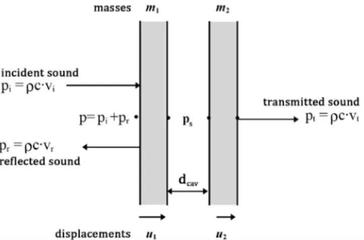
Similar to single-leaf homogeneous walls, the sound insulation of a cavity construction can be theoretically predicted by a mass law. For the derivation of this mass law an identical approach as for single-leaf walls can be followed. Figure 4.2 schematically presents the acoustic model for airborne sound transmission through a cavity construction for normal incidence of sound waves. Coincidence effects can then thus be neglected. This model is a simplified version of reality since we assume that the cavity construction has infinite dimensions in length and width. Besides, we assume that the leaves on both side of the cavity are infinitely stiff so that no bending of these leaves takes place (piston model). Moreover, we assume that no pressure gradient in the cavity exists. Implicitly we thus assume that the cavity is much smaller than the wavelength of the incident sound.
However, the pressure inside the cavity can vary; if the width of the cavity is relatively small1, the air inside
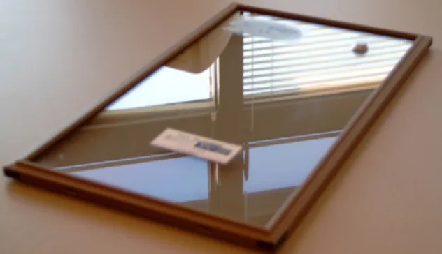
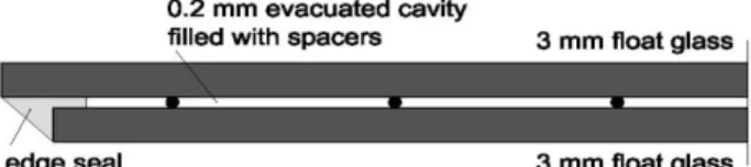
Figure 4.1 – Example of a cavity construction: vacuum insulation glass.
1 If the width of the cavity is relatively large, the air layer no longer acts as spring. In that situation the air cavity more
Figure 4.2 - Cavity model for normally incident acoustic waves.
the cavity acts as a spring which can be compressed and stretched. According to Hooke’s law, we can write for the pressure inside this spring, ps
(
1 2)
cav s cav cav d E p E u u d d ∆ = − = − (4.1), In this equationE = the compression or Young’s modulus of the spring (E =1.4·105 Pa for an air spring)
dcav = the width of the cavity [m]
u1, u2 = the displacement of the leafs [m].
According to Newton’s second law of motion, we can write for each of the leafs 2 1 1 2 s u p p m t ∂ − = ∂ (4.2a), 2 2 2 2 s t u p p m t ∂ − = ∂ (4.2b), with
m1, m2 = the mass of leaf 1 and 2 respectively [kg/m2]
t = time [s]
p = the sum of the pressure of the incident and reflected sound wave [Pa]
pt = the pressure of the transmitted sound wave [Pa].
Since the leaves are assumed to be infinitely stiff, we can write for the left and right leaf
(
)
(
)
1 1 1 2
i r i r i
air air air air
u v v p p p p t ρ c ρ c ∂ = − = − = − ∂ (4.3a), 2 t t air air u v p t ρ c ∂ = = ∂ (4.3b), with
vi = the vibration speed of air molecules of the incident sound wave [m/s]
vr = the vibration speed of air molecules of the reflected sound wave [m/s]
vt = the vibration speed of air molecules of the transmitted sound wave [m/s]
From the previous equations, u1, u2, p and ps can be eliminated resulting in the following differential equation
(
)
2 2 2 3 1 2 1 2 1 2 2 3 2 2 2 cav air air cav t t cav t i tair air air air
d m m c p m m d p m m d p E p p c t E t c E t ρ ρ ρ + + ∂ + ∂ ∂ = + ∂ + + ∂ ∂ (4.4).
In this equation ρ2airc2airdcav/E is negligible relative to m1 + m2. In a similar way as for a homogeneous wall, the ratio of the amplitudes of pi and pt can now be computed for a certain frequency as
(
)
ω ω ω ρ = = − + + + − 2 2 2 2 ;max 2 2 1 2 1 2 1 2 2 ;max 1 1 2 2 i cav cav air air t p m m d m m m m d t p E c E (4.5), witht = the sound transmission coefficient through the cavity construction [-] ω = the angular frequency of the acoustic wave (=2πf) [rad/s].
This formula shows that the transmission coefficient has a maximum at that frequency where the last term on the right side of the equation is zero. This occurs at the so-called (angular) frequency of mass-spring resonance for normal incidence of sound waves (section 4.3), ωms⊥ (=2πfms⊥)
(
1 2)
1 2 ms cav m m E m m d ω ⊥= + (4.6),For sound hitting the construction with an angle θ from the normal of the plane, the component of vi, vr and
vt along this normal should be used in equations (4.3a) and (4.3b). Equation (4.5) then changes in such a way that ω·cosθ should be used in stead of ω. Using equation (4.6), this general equation can elegantly be
written as
(
)
ω ω(
)
ω θ θ θ ρ ω ⊥ ω ⊥ + + = = − + − 2 2 2 2 2 2 2 1 2 1 2 ;max 2 2 2 2 2 1 2 ;max1 1 cos cos 1 cos
2 2 i air air t ms ms m m m m p t p m m c (4.7).
Since the airborne sound insulation of a partition wall or a façade was defined using this transmission coefficient, we can finally write for the airborne sound insulation of a double-leaf cavity construction
(
)
2 2 2(
)
2 2 21 2 2 1 2 2
; 2 2
1 2
10log 1 cos cos 1 cos
2 2 cav ms air air ms m m m m R m m c θ ω ω θ θ ω θ ω ⊥ ρ ω ⊥ + + = − + − (4.8).
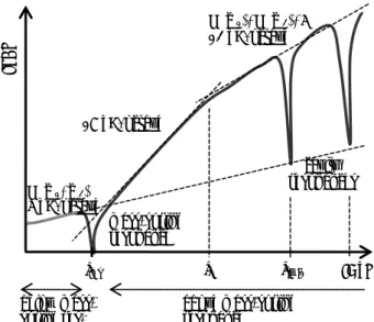
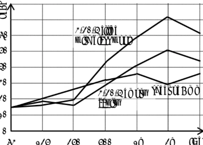
From this general equation, called the theoretical mass law for cavity constructions, the general behaviour of the airborne sound insulation of such constructions can be explained in detail. This general behaviour is shown in Figure 4.3. As can be seen, we can distinguish between several frequency regions which will each be treated separately in the next sections: below mass-spring resonance, at mass-spring resonance and above mass-spring resonance. Besides this behaviour reflected by the mass law, three additional effects will be discussed: standing waves inside the cavity (cavity resonances), the influence of couplings between both leaves and the influence of sound absorption material inside the cavity.
Figure 4.3 – General frequency-dependent behaviour of cavity constructions.
4.3
Mass-spring resonance
As seen in the previous section, at a certain frequency the transmission coefficient has a maximum. As a consequence, the airborne sound insulation has a minimum at this frequency. The airborne sound insulation then follows from substituting ωms⊥/cosθ for ωin equation (4.8) resulting in
1 2 ; 2 1 20log 2 2 cav ms m m R m m = + (4.9).
This equation interestingly shows that the airborne sound insulation of a symmetrical cavity construction, i.e. m1 = m2, becomes 0 dB. This minimum can be somewhat increased by adding a porous absorption material, like mineral fibre insulation inside the cavity. Then, the minimum slightly increases and spreads over a larger frequency interval; it becomes less pronounced. Near mass-spring resonance the sound insulation is thus very low. The reason is that both leaves then move in counter-phase as a result of which vibrations are easily transferred.
Since mass-spring resonance of a cavity construction is a general mass-spring resonance phenomenon with two masses and one spring, the frequency where this phenomenon occurs follows from2
1 2 1 ' 1 1 2 cos ms t f s m m π θ = + (4.10a),
with s’t [N·m-3] the stiffness of the spring. This stiffness is defined as Young’s (or compression) modulus divided by the thickness of the spring while the compression modulus of air equals ρ0c20. Provided that the cavity is filled with air, we can thus write for the frequency where mass-spring resonance occurs as
2
1 2 1 2
1 1 1 1 1
2 cos air air 2 cosair air
ms cav cav c c f d m m d m m ρ ρ π θ π θ = + = + (4.10b).
2 The mass-spring resonance frequency for random incidence of sound waves can be estimated using an angle of incidence
of around 60o to 65o. f [Hz] R [d B] cavity resonances 12 dB/octave mass-spring resonance 6 dB/octave R (m1+m2) R (m1)+R (m2)+6 18 dB/octave fms fT fsw;1 below
mass-spring res. above mass-spring resonance
Figure 4.4 - Influence of angle of incidence on the mass-spring resonance frequency (double-glazing 6-30-6). As seen from this equation, the angle of incidence of the sound wave influences the mass-spring resonance frequency. For normal incidence (θ=0o) this frequency is lowest and it increases for increasing angle of incidence. Figure 4.4 presents this behaviour graphically. This also implies that in case of random incidence, i.e. sound waves are coming from practically all directions, the resonance dip is not sharp and small but shallow and extended over a wide frequency range. The lowest value mostly also moves to a ½ to 1 octave higher frequency.
If we now finally fill in the values for ρair (1.21 kg·m-3 at 20oC) and cair (=343 m·s-1 at 20oC) and assume normal incidence of sound waves (θ=0o), we can write equation (4.10b) as
1 2 1 2 60 ms cav m m f m m d ⊥ + ≈ (4.10c).
The dip due to mass-spring resonance closely resembles the dip during coincidence for single-leaf walls. The phenomena however differ from each other. Coincidence is a phenomenon involving bending waves inside a plate, mass-spring resonance involves stretching and compression of the cavity for which the cavity leaves were assumed to have infinite bending stiffness. So, both phenomena should not be confused. We have seen that near mass-spring resonance the airborne sound insulation of a cavity construction is low. It is particularly important that fms does not lie between 200 and 2000 Hz. If fms is higher than 2000 Hz, the advantage of a cavity construction over a single-leaf wall is no longer available. Therefore cavity constructions should be designed in such a way that fms < 200 Hz or even better fms < 100 Hz.
4.4
Sound insulation below mass-spring resonance
The mass law for cavity constructions (equation (4.8)) can be simplified for ω < ωms/2, i.e. for the frequency region below mass spring resonance. Here, this mass law can be approximated as
(
)
2 1 2 ; cos 10log 1 2 cav air air m m R c θ ω θ ρ + = + (4.11a). f [Hz] 63 125 500 1k 2k 4k 89O 0O 30O R [d B] 20 40 60 80 100 0 250 8kSince most cavity constructions in buildings have leaves with relatively high mass, this equation can even be further simplified to
(
1 2)
; cos 20log 2 cav air air m m R c θ ω θ ρ + ≈ (4.11b).This equation closely resembles the mass law for single-leaf homogeneous walls with as difference that the total mass of both leaves should be taken in stead of the mass of the homogeneous wall. In fact, below mass-spring resonance a cavity construction thus acoustically performs as a homogeneous wall of equal mass
; sin ;( 1 2) cav gle
R θ≈R θ m m+ (4.12).
These equations clearly demonstrate that below mass-spring resonance the airborne sound insulation of a cavity wall increases with 20 log ω = 6 dB per octave but also with 6 dB per doubling of total mass m1+m2. In
this frequency range, the airborne sound insulation of a cavity construction approximately equals the airborne sound insulation of a single-leaf homogeneous wall of identical mass.
In practice, however, especially inside buildings, the sound field is diffuse. As a consequence, acoustic waves hitting the cavity construction have multiple directions. We assume that all directions, thus all angles of incidence, are equally and simultaneously present in the sound field in front of the construction. To obtain the airborne sound insulation for such random incidence, we must average equation (4.11b) over all angles of incidence within half a sphere. Ten times the logarithm of the average of cos2θ equals
/2 /2
2 2
0 0
1 1
10log cos 10log 2 sin cos 5
2 d 2 d π π θ π θ θ θ π π Ω = ≈
∫
∫
(4.13).Similar to a homogeneous wall, the airborne sound insulation of a cavity wall for random incidence equals its airborne sound insulation minus approximately 5 dB
; ; 5
cav random cav
R ≈R ⊥− (4.14).
4.5
Sound insulation above mass-spring resonance
The mass law for cavity constructions (equation (4.8)) can be simplified for ω > 2ωms as well, i.e. for the frequency region above mass-spring resonance. Here, this mass law can be approximated as
3 3
1 2 ; 20log 2 2cav3cos cav air air m m d R c θ ω ρ θ = (4.15a).
As can be seen, in this high frequency region, the airborne sound insulation of a cavity construction depends on both masses of the leaves and on the width of the cavity; the wider the cavity, the higher the airborne sound insulation is. Equation (4.15) can also be re-arranged and written in a different form as
1 2
; 20log 2 cos 20log 2 cos 20log 2 cavcos cav
air air air air air
m m d R c c c θ ω θ ω θ ω θ ρ ρ = + + (4.15b),
clearly showing the influence of each of the three components: mass of leaf 1, mass of leaf 2 and cavity width. Apparently, the airborne sound insulation equals the sum of the individual sound insulations of each leaf, reflected by a mass law equal to the one for a homogeneous wall, plus an additional bonus from the cavity
; sin ; ( )1 sin ;( ) 20log2 2 cavcos
cav gel gel
air d R R m R m c θ θ θ ω θ = + + (4.16).
Above the mass-spring resonance frequency, the airborne sound insulation of a cavity wall (first) increases with 60 log ω = 18 dB per octave in stead of 6 dB per octave in case of single-leaf walls. In this frequency range, the airborne sound insulation of a cavity construction approximately equals the sum of the individual airborne sound insulation values of each leaf plus a bonus coming from the cavity. This increase of 18 dB per octave is the big plus of a cavity construction over a single-leaf wall.
In a similar way as done in section 4.4 for constructions below mass-spring resonance, we can derive an approximation for the sound insulation of a cavity wall above mass-spring resonance in case of random sound incidence. We again assume that all directions, thus all angles of incidence, are equally and simultaneously present in the sound field in front of the construction. To obtain the airborne sound insulation for such random incidence, we must now average equation (4.15a) over all angles of incidence within half a sphere. Ten times the logarithm of the average of cos6θ equals
/2 /2
6 6
0 0
1 1
10log cos 10log 2 sin cos 8.5
2 d 2 d π π θ π θ θ θ π π Ω = ≈
∫
∫
(4.17).So, the airborne sound insulation of a cavity wall for random incidence above mass-spring resonance equals its perpendicular airborne sound insulation minus approximately 8.5 dB
; ; 8.5
cav random cav
R ≈R ⊥− (4.18).
According to equation (4.16) it would now seem as if the airborne sound insulation resulting from the cavity always increases with increasing frequency. Practice has however shown that this is not the case and that the maximum of the cavity term of equation (4.16) is limited to approximately 6 dB. This maximum is thus reached at a certain frequency, fT, for which
2(2 ) cos 20log T cav 6 air f d c π θ = (4.19a),
or, rewritten in a different form, for which holds
2 aircos T cav c f d π θ = (4.19b).
If we finally take an angle of incidence of 60o as a reference for random incidence, we get for the transition frequency in case of random incidence
; 2 air/2 air T random cav cav c c f d d π π = = (4.19c).
From this frequency onwards, the cavity term of equation (4.16) thus no longer increases with frequency and its airborne sound insulation equals
; sin ;( )1 sin ; ( ) 62
cav gle gle
R θ=R θ m +R θ m + (4.20).
This equation can easily be extended to three or more leaves if needed; each leaf adds Rsingle (mi); each cavity adds 6 dB. Be aware that this only holds for frequencies above fT for all cavity systems.
Above the transition frequency fT, the airborne sound insulation of a cavity wall increases with 40 log ω = 12
dB per octave. In this frequency range, the airborne sound insulation of a cavity construction approximately equals the sum of the individual airborne sound insulation values of each leaf plus 6 dB (for each cavity).
In practice however this maximum value of 6 dB is hardly ever reached because of three reasons. First, the air cavity is not a simple spring but an air volume. In this air volume a 3D pattern of standing sound waves might occur, of which the most important are the standing waves perpendicular to the main surface of the leafs. Such standing waves reduce the airborne sound insulation of cavity constructions (at higher frequencies) in a small frequency range. This effect is further explained in the next section. Second, sound absorption inside the cavity influences the system’s airborne sound insulation particularly where resonance phenomena (mass-spring resonance and standing waves) occur. The influence of sound absorption of elaborated in section 4.8. Third, coincidence effects in each leaf might reduce the airborne sound insulation as well. If however the thickness of each leaf is different or they are made of different materials, a dip due to coincidence in one leaf might be masked by the other leaf. The coincidence phenomenon has already been extensively explained in chapter 3.
4.6
Standing waves inside the cavity
In the previous sections, the classical approach to solving sound transmission through cavity constructions was explained. This approach can be complemented, particularly for situations in which the classical approach is not valid, with an approach called ‘statistical energy analysis’ (SEA). We now distinguish between non-resonant transmission which is described by the classical approach and resonant transmission which is described by SEA. In the lower frequency domain, non-resonant transmission dominates and the equations described in the previous sections can be used. In the higher frequency domain, resonant transmission dominates and the SEA method should be used.
The SEA approach, which is based on a statistical approach, describes a sound or vibration field as a set of resonance frequencies called resonance modes or simply modes. Sound transmission from an air space (room) to a construction element and vice versa is now described as transmission of acoustic power from a mode in one system with frequency fn to a mode in the other system with frequency fm. Sound transmission can however only occur if fn is close to fm and the coupling between both elements is high. High sound transmission from one element to the other can thus only occur if the number of resonance modes per octave band is high; then the likelihood that fn and fm are close together is high.
In general, the higher the frequency is the higher the number of resonance modes per frequency band, N, is:
in a room: N ~ f3
in a cavity with approx. dcav > λ / (π√2): N ~ f3 in a cavity with approx. dcav < λ / (π√2): N ~ f2
in a plate: N ~ f
This overview above gives an interesting observation. If the wavelength of the sound decreases to below a certain value, which for random incidence approximately equals π√2dcav, or in other words if the frequency
of the sound increases to beyond a certain value, then the number of modes per frequency band starts to more rapidly increase with frequency. This observation explains why at higher frequencies, i.e.
approximately above fT, the increase of Rcav with frequency drops from 18 dB/oct. to 12 dB/oct.
If there is no acoustic dampening of the resonance modes inside the cavity (because of sound absorption material), vibrations with large amplitudes occur if fn and fm are close together. The cavity leafs are then acoustically coupled, as a result of which the construction acts as a single-leaf wall of identical mass. The frequencies where such cavity resonances, or standing waves, occur can be calculated from
sw n; 2 air cav nc f d = (4.21a), with
n = a random integer representing the order of the frequency mode (n = 1, 2, 3, 4, etc.).
At or around this frequency the cavity construction thus experiences a sharp drop in its sound insulation value, Rcav, as can be seen from Figure 4.3. In a very narrow frequency range around fsw;n, the cavity construction acts
as a single-leaf wall with identical mass. As a consequence, Rcav drops to the equivalent value of such a
single-leaf wall. The plateau method for single single-leaf walls, which is explained in the previous chapter, can be used to estimate the value of Rcav at fsw;n.
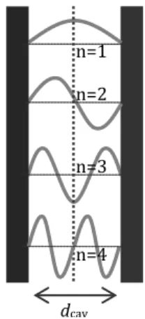
From a classical perspective, the previous phenomenon of cavity resonances can be explained as
the occurrence of standing waves inside the cavity. Such standing waves for instance also occur
in a vibrating guitar string or in an organ pipe. In a closed air cavity, air particles near the leaves
cannot vibrate because they are restricted in their movement. As a result, standing waves inside
the cavity in a direction perpendicular to the leaves can only occur if an acoustic wave fits inside
the cavity in such a way that the width of the cavity equals n-times half a wavelength as can be
seen from Figure 4.5. Or mathematically written
; 2sw n cav n
d = λ (4.21b).
With λ = cair / f this equation can be re-written as equation (4.21a). Standing waves thus lie beyond the transition frequency. As will be discussed in the next section, standing waves can easily be dampened using sound absorption material inside the cavity. Such sound absorption material, by the way, does not always have to be filling the entire cavity. In case of double-glazing it can also be placed along the rim of the system.
Figure 4.5 – Standing waves of different modalities (n=1, 2, 3 and 4) inside an air cavity.
dcav n=1 n=2 n=3
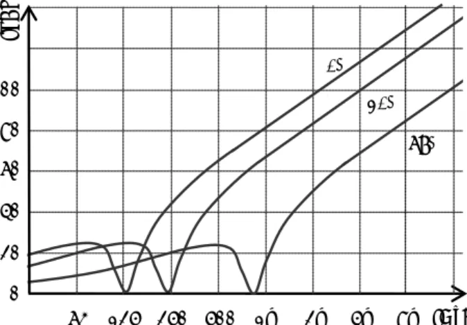
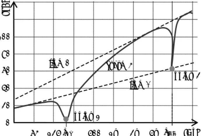
Figure 4.6 -Construction of the curve of the sound resistance of two glass sheets of 3mm and 4 mm separated by an air cavity of 20 mm.
4.7
Constructing an insulation curve, mass versus width and oblique incidence
4.7.1 The construction of an insulation curve
Figure 4.6 illustrates an initial approximation of the sound resistance of a cavity construction for normal
incidence (i.e. no coincidence). The example assumes two glass sheets of 3 mm and 4 mm with a cavity of
20 mm. The following steps can be used to construct the sound insulation curve of this construction: 1. Construct in a figure with a logarithmic frequency axis a straight line for a single-leaf construction with
a mass identical to that of the cavity construction: here 3 + 4 = 7 mm glass. This line increases with 6 dB/oct. Use equation (4.11b). This curve now represents the minima that we encounter in cavity resonances and the sound resistance that we see at extremely low frequencies.
2. Construct in the same figure a straight line for the cavity construction at very high frequencies (above
fT). It goes without saying that this curve now rises with 12 dB/oct. in stead of 6 dB/oct. Use equation (4.20).
3. Calculate the frequency where mass-spring resonance occurs in accordance with equation (4.10b) and determine the airborne sound insulation of the cavity construction at this frequency according to equation (4.9). Mark this value in the figure.
4. Calculate the frequencies at which the cavity resonances produce minima in accordance with formula (4.21a) and mark the positions of these frequencies on line (1).
5. Using the values obtained, the curve of Rcav can now be drawn: the curve starts at extremely low frequencies at line (1); falls sharply around the mass-spring resonance frequency towards point (3); then rises sharply first with 18 dB/oct. and then with 12 dB/oct. towards line (2); and subsequently oscillates between the maximum (line (2)) and minimum (line (1)) lines where cavity resonances occur.
It may be concluded from Figure 4.6 that for normal incidence, a 3-20-4 cavity construction performs better above approximately 300 Hz than a single 7 mm sheet of glass.
4.7.2 Increasing mass versus increasing cavity width
The weakest point of the 3-20-4 construction mentioned in the section above is that the mass-spring resonance occurs around 200 Hz, which is exactly in the sensitive zone for speech (for partition walls) and
f [Hz] fms fsw;1 R [d B] 20 40 60 80 100 0 63 125 500 1k 2k 4k line (1) line (2) point (3) point (4) curve (5)
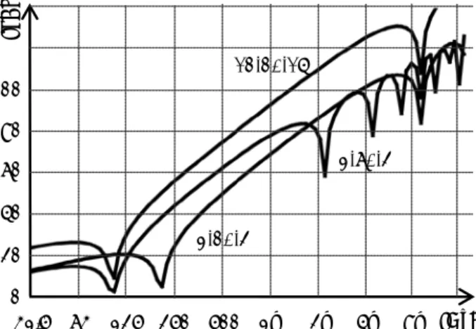
Figure 4.7 - Comparison of three glass cavity constructions.
traffic noise (for external walls). Figure 4.7 shows an example in which an attempt is made to improve the sound resistance by quadrupling either its mass, or the thickness of its cavity. Quadrupling either mass or cavity thickness leads, for normal incidence, to a reduction of the mass-spring resonance frequency by half. Outside this frequency band, increasing the mass is more effective than making the cavity thicker.
However, the improvement achieved by widening the cavity is also considerable in the zone between 125 Hz and 1000 Hz, so that a compromise will often be chosen.
4.7.3 Cavity construction for oblique and uniformly distributed incidence
It was observed in the previous chapter that the sound insulation of a single sheet decreases by
approximately 5 dB for random incidence compared to perpendicular incidence. This effect naturally also plays a role in cavity constructions, however, alongside a second effect: both the mass-spring resonance frequency and the cavity resonance frequencies shift to higher values in case of oblique (and also random) incidence. This becomes evident from the cosine term in for instance equation (4.10a). As can be seen from Figure 4.8, the effect is stronger for mass-spring resonance than for standing waves inside the cavity.
Figure 4.8 - The calculated sound resistance at various angles of incidence for a cavity construction consisting of two glass sheets of 3 mm and 4 mm with an air cavity of 20 mm. In order to clearly illustrate the shifts in the minima, the
f [Hz] R [d B] 20 40 60 80 100 0 63 125 500 1k 2k 4k perpendicular 8k 250 30o 60o 31.5 75o 89o f [Hz] R [d B] 20 40 60 80 100 0 63 125 500 1k 2k 4k 12-20-16 8k 250 3-20-4 3-80-4 31.5
f [Hz] R [d B] 10 20 30 40 0 125 250 500 1k 2k 63 perpendicular incidence random incidence 50 60 f [Hz] R [d B] 10 20 30 40 0 125 250 500 1k 2k 63 3-20-4 filled with glass wool
Sheet of 7 mm 50
60
3-20-4 empty cavity
Figure 4.9 - The sound resistance of a 3-20-4 cavity construction for normal and uniformly distributed (=random) incidence. The normal curve is equal to that in the previous figure, but the calculation is now in octaves.
Figure 4.10 – The sound resistance of three constructions. A glass wool filling in the cavity dampens the vibrations at near mass-spring resonance, thus increasing the sound insulation.
The shift of the cavity resonances for glass constructions is usually favourable. At 0° and 30° they are still visible at around 8 kHz, but as the angle of incidence increases, the dips move to a value beyond 16 kHz. On the other hand, the shift of the mass-spring resonance is generally unfavourable. It shifts towards a
frequency range where acoustic nuisance can be particularly annoying.
Figure 4.9 shows how utterly detrimental this influence can be. The figure presents a calculation of the cavity construction for normal and uniformly distributed incidence, showing a difference of 20 dB or more from 500 Hz onwards. This situation contrasts sharply with the differences between normal and uniformly distributed incidence for a single sheet, where a difference of approximately 5 dB is observed.
4.8
Sound absorption inside the cavity and gas-filled or evacuated cavities
4.8.1 Sound absorption - normal incidence
When resonance occurs in a cavity, whether of the mass-spring or standing wave variety, the ‘air’
molecules make large excursions around their equilibrium position. The sound resistance can be improved by limiting the amplitude of these excursions. In practice this is nearly always achieved using a material that absorbs sound, which is to say one in which considerable friction occurs because the air is vibrating
within narrow openings. Glass wool is an example of a sound-absorbing material of this kind3. Synthetic foams also absorb well provided the material has many open cells. Expanded polystyrene does not meet this condition, and is therefore not a good acoustic material.
Figure 4.10 gives an example that compares three constructions, and shows that a glass wool filling, for
normal incidence, indeed improves the sound resistance near mass-spring frequency; the minimum is
raised somewhat. However, the figure also shows that for these particular constructions the single 7 mm sheet, having identical mass as the cavity constructions, performs even better than both cavity
constructions up to 300 Hz.
Application of a sound absorption material, like mineral fibre board, inside the cavity of a cavity construction improves the sound insulation of this construction near mass-spring resonance and near the frequency where standing waves occur; the dip becomes less deep and spreads over a wider frequency range. Particularly at higher frequencies porous absorbers can be very effective; for lower frequency absorption Helmholz
resonators are more effective. The material used as absorption however should not stress the leaves; should be less stiff than an equally thick air layer; should absorb sound; and should not reduce the effective cavity width. Mineral fibre absorption works well; hard polymer foams like Polystyrene however can be detrimental. 4.8.2 Sound absorption - oblique and uniformly distributed incidence
Suppose a wave impinges on a cavity construction at an angle of 60°. This wave, like an optical system, is then refracted in the sheet and refracted back to 60° in the cavity. This angled wave can always be deemed to be resolved into a wave perpendicular to the construction, i.e. a ‘normal’ wave, and one parallel to the cavity construction, i.e. a ‘lateral’ wave. The normal wave obviously propagates only for a short distance, i.e. the width of the cavity, but the lateral wave may travel as far as one metre through the cavity. As a result, a glass wool filling has many times a greater effect on lateral waves than on normal waves, so that a glass wool filling bends the angle of 60° back to the normal considerably.
This effect can be extremely favourable. We have seen that the differences between normal and oblique incidence was very considerable for a cavity construction (Figure 4.9), so that the sound resistance of a cavity construction would increase substantially if we were able to make uniformly distributed incidence resemble normal incidence. Apparently, a glass wool filling appears to go some way in that direction. The
Figure 4.11 - The effect of glass wool filling for random incidence. The coincidence effect is factored in here. 3 Glass wool is commonly referred to as an ‘insulation material’, but acoustically speaking the term is wrong. A sheet
f [Hz] R [d B] 10 20 30 40 0 125 250 500 1k 2k 63 3-20-4 filled with glass wool 50 60 3-20-4 empty cavity sheet of 7 mm
Figure 4.12 - Typical cross-section through vacuum insulation glass.
effect is demonstrated in Figure 4.11. The glass wool filling results in an improvement of more than 10 dB, in particular at the higher frequencies. Compare the curve with the normal incidence of Figures 4.9 and 4.10. It will be evident that a glass wool filling between two glass sheets is seldom applied in practice. Glass wool fillings are used mainly for partition constructions, for example with plasterboard cavity walls.
4.8.3 Gas-filled and evacuated cavity
Special gases heavier than air, e.g. argon and krypton, are sometimes used for double-glazing. The main reason is improved thermal performance, but the gas filling also has some acoustic benefits. If a wave impinges at 60°, the angle in the gas-filled cavity is less than 60°. This means that, like in case of glass wool, the curve for random incidence shifts towards that of normal incidence. However the effect observed with a heavy gas is never as big as for glass wool. Furthermore, a gas filling lacks the attenuation of the mass-spring resonance, so that the sound resistance of a heavy gas is often less than that of air.
Another interesting point is that a gas lighter than air has a positive impact on sound resistance. It is beyond the scope of this chapter to provide a physical explanation of this phenomenon. Moreover light gases like helium are never used in practice; helium would leak too easily from a construction.
However, vacuum constructions have been produced in practice, and they also have a favourable effect. This is best illustrated by Equation (4.10a) and (4.10b). The value of cair remains unchanged in theory but for ρair a value must be entered proportional to the actual cavity air pressure. The stiffness of an air cavity,
s’t, equals ρgas·c2gas/dcav or written differently γ·pgas/dcav with γ the ratio of the specific heat at constant volume to the specific heat at constant pressure (=1.4 for air) and pgas the gas pressure inside the cavity. If the gas pressure is now reduced, the stiffness of the cavity reduces and consequently mass-spring
resonance shifts to lower frequencies. For a conspicuous effect, though, the pressure must be pumped to below 0.1 bar. The forces on the leaves of a vacuum cavity are extraordinarily high (105 N/m2) and therefore demand the use of spacers inside the cavity (Figure 4.12), which have the great disadvantage of forming an acoustic coupling between the cavity leaves, lowering the sound resistance again. The
application of rubber blocks is of no help because the rubber would be compressed so powerfully that little or nothing would remain of its spring properties.
4.9
Structural couplings between leafs
4.9.1 Theoretical considerations
If structural couplings between the leaves, like cavity ties, are in place, both leaves are connected to one another. Such couplings may reduce the sound insulation of a cavity construction. The extent to which they have an influence depends on three factors:
• the type of coupling: point or line coupling;
• the flexibility of the coupling: rigid or flexible coupling; • the number of couplings per m or per m2.
Flexible couplings hardly transfer any sound via the coupling from one leaf to the other. If their number is limited, they hardly influence the sound insulation of a cavity construction.
Rigid couplings however structurally connect the two leaves. As a result, the vibration velocity of each cavity leaf near the coupling is identical. Since they here move simultaneously and with identical velocity, the behaviour of the cavity wall near the coupling is similar to a single-leaf wall with identical mass. Although the connection between the two leaves is highly localised to the spot of the coupling, its influence reaches further than this localised spot. Around the coupling there exists a small zone, or area, where the influence of the coupling is felt. The size of this zone depends on the bending stiffness of the cavity leaves. Since the coincidence threshold frequency also depends on bending stiffness, we can express the size of this zone as function of the threshold frequency for coincidence, fg, as explained in chapter 3. According to Martin (2007) we can then write
2 2 2 3 3 g air coupling g c S f λ
= = for a point-like connection (4.22a),
2 2
3 3
coupling g coupling air coupling g l l c S f λ
= = for a line-like connection (4.22b),
with
λg = the wavelength of the sound when coincidence starts occurring [m];
lcoupling = the length of the line coupling [m].
Note that equations (4.22a) and (4.22b) give the surface area around one single coupling. If there are multiple couplings, these areas need to be multiplied with the number of couplings to get the total area that acts as a single-leaf wall.
A cavity construction with rigid couplings can now be considered as a composite wall with a surface area Stot -
Scoupling that behaves as a cavity construction and a surface area Scoupling that behaves as a single-leaf wall with
identical total mass as the cavity construction. The total sound insulation of this system can for each frequency band be calculated with the equation for composite walls as discussed in chapter 2.
We thus get for the total sound insulation of the cavity construction with rigid connections
sin /10 /10
10log tot coupling10Rcav coupling10R gle composite tot tot S S S R S S − − − = − + (4.23a).
If Rcav becomes much bigger than Rsingle, which is the case far above the mass-spring resonance frequency, this equation can be simplified to
sin 10log tot composite gle coupling S R R S = + (4.23b).
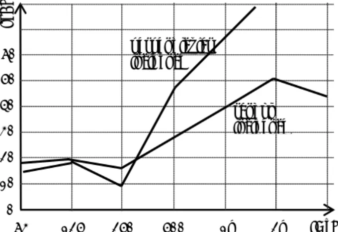
From this last equation we can learn that far above mass-spring resonance the coupled part of the construction dominates the sound transmission through the façade. As a result, the increase of the airborne sound insulation is only 6 dB/oct. compared to 18 or 12 dB/oct. for an uncoupled cavity construction. Moreover, in this high frequency range, the gain of a coupled cavity construction over a single-leaf wall is determined by the ratio of the total to the coupled surface area. Figure 4.13 gives an example of the influence of contact bridges in a cavity construction on airborne sound insulation.
Based upon equation (4.23b) so-called nomograms can be produced which allow a rapid estimation of the increase in sound insulation of a coupled cavity construction compared to a single-leaf wall of equal mass,
Figure 4.13 – Airborne sound insulation of a cavity construction of two 6 mm thick plywood leaves and a cavity of 60 mm filled with mineral fibre insulation. Top line: cavity without couplings; middle line: cavity with wooden couplings 60x60 mm2 with a distance of 800 mm; bottom line: single-leaf 12 mm thick plywood. Data taken from Martin (2007).
Figure 4.14a – Improvement of the airborne sound insulation of a coupled (point-like couplings) cavity construction compared to an equally heavy single-leaf wall. Parameter along the lines is the threshold frequency for coincidence of
the cavity leaves. Source: Martin (2007).
Figure 4.14b – Improvement of the airborne sound insulation of a coupled (line-like couplings) cavity construction compared to an equally heavy single-leaf wall. Parameter along the lines is the threshold frequency for coincidence of
4.9.2 Practical considerations
In practise a connection between the cavity leaves occurs rather often. Such couplings can either be wanted connections or unwanted connections. In general unwanted connections are a result of design or construction errors. The occurrence of unwanted connections can thus be limited by good design and careful construction. Examples of unwanted connections are:
• mortar which gets inside the cavity due to careless bricklaying or a too small cavity;
Mortar inside the cavity can be prevented by putting mineral fibre insulation in the cavity during bricklaying.
•
ducts through the wall with rigid connections to both leaves;Connections caused by ducts can be prevented by using flexible pipes and by filling the pipe holes around the duct with flexible material.
• rigid polymeric foam insulation foamed into the cavity after construction;
The connection resulting from polymeric foams inside the cavity in practise hardly ever causes problems since windows and ventilation openings in the façade are the weak spots from the perspective of sound insulation. In case of walls that partition two dwellings, soft mineral fibre insulation should be used in stead if thermal requirements are in place.
Wanted couplings mostly have a structural function. They are thus needed. Very often such couplings are rigid connections significantly influencing the airborne sound insulation of the cavity construction. From an acoustical perspective a better way is making them flexible. However, acoustical requirements, cost and other practical considerations must be balanced to find the right solution. Examples of wanted connections are:
• cavity ties used with masonry cavity walls (around 4 per square meter);
Because normal masonry cavity walls have around 4 ties per square meter they acoustically do not behave as a cavity wall but as a single-leaf wall with identical mass.
• lathes inside a lightweight interior wall;
Lathes inside lightweight interior walls are mostly rigidly connected to both leaves because of wanted rapid mobility. From an acoustical perspective it is however preferred to split the system of laths into two parts as can be seen from Figure 4.15.
• lathes behind a lightweight flexible secondary wall.
A flexible secondary wall is often (rigidly) connected to a homogeneous wall because of low cost. This is however hardly ever needed. Good but more expensive alternatives are to connect the secondary wall to the floor and ceiling alone using its own supporting structure or to use flexible connections. Figure 4.16 gives some examples of connections. It is however important to realise that the sound transmission via couplings is complex and can sometimes be counter-intuitive. For a very flexible secondary wall, a coupling via a heavy steel section can for instance be better than via a thin and lightweight strip.
Figure 4.16 – Vertical cross-section through the connection of a secondary wall to a homogeneous wall. Left: rigid line connection; middle: rigid point connection; flexible point connection.
4.10 Triple layered systems: mass-spring resonance
Up till now we have only discussed double layered systems, i.e. systems having two masses (leaves) and one cavity. In practise however facades or walls with many more layers exist as well. Most of these systems can no longer be easily calculated using analytical models; in stead therefore computer model, like the multi layer model, are used. However, there is an analytical equation with which the mass-spring resonances of a triple layered system can be computed. This equation is thus valid for walls and facades having three leaves (masses) and two cavities, a so-called mass-spring-mass-spring-mass system. The two mass-spring resonance frequencies, one for each cavity, can be determined from (Blevins, 1979):
2 1 2 1 2 1 2 1 2 ;1 1 2 2 1 3 2 1 3 1 2 2 3 1 3 1 ' ' ' ' ' ' ' ' 4 ' ' 1 1 1 2 2 msmsm s s s s s s s s f s s m m m m m m m m m m m m π + + = + + − + + − + + (4.24a), 2 1 2 1 2 1 2 1 2 ;2 1 2 2 1 3 2 1 3 1 2 2 3 1 3 1 ' ' ' ' ' ' ' ' 4 ' ' 1 1 1 2 2 msmsm s s s s s s s s f s s m m m m m m m m m m m m π + + = + + + + + − + + (4.24b),
With s’1,2 [N] the stiffness of cavity one and two respectively. For an air cavity this stiffness is calculated as 2 ' air air cav c s d ρ = (4.25).
It should be noted however that generally only the first resonance is noticeable.
4.11 Practical considerations
Read chapter 12 Applied Sound Insulation from the book ‘Building Physics’ by A.C. van der Linden. 4.11.1 uncoupled cavity walls
4.11.2 flexible secondary walls
4.11.3 mobile lightweight partition walls 4.11.4 double glazing
4.11.6 suspended ceilings
4.11.7 wooden floor constructions
4.12 Design Guidelines and Construction Errors
Read chapter 12 Applied Sound Insulation from the book ‘Building Physics’ by A.C. van der Linden.
4.12.1 Design guidelines 4.12.2 Construction errors
4.12 Literature
Blevins.. (1979) …Braat-Eggen, P.E. and Luxemburg, L.C.J. van (1993), Geluidwering in de woningbouw, Thieme Meulenhoff. Martin, H.J. (2007), Geluidisolatie, lecture notes for the course Acoustics 7S510, Eindhoven University of
Technology, Eindhoven.
Nederlof, L. and Cauberg, J.J.M. (2005), “Module A18: Luchtgeluidisolatie van spouwconstructies”, In: Kennisbank Bouwfysica, Stichting Kennisbank Bouwfysica.
Vér, I.L. and Beranek, L.L. (2005), Noise and Vibration Control Engineering: Principles and Applications, John Wiley & Sons, Hoboken.