Local air pollution and global climate change: a combined cost-benefit analysis

(1)

Netherlands Environmental Assessment Agency (MNP), P.O. Box 303, 3720 AH Bilthoven, the Netherlands; Tel: +31-30-274 274 5; Fax: +31-30-274 4479; www.mnp.nl/en

MNP Report 500116002/2007

Local air pollution and global climate change

A combined cost-benefit analysis

J.C. Bollen, B. van der Zwaan, H.C. Eerens, and C. Brink

Contact:

Johannes Bollen MNP/KMD jc.bollen@mnp.nl

(2)

Parts of this publication may be reproduced, on condition of acknowledgement: 'Netherlands Environmental Assessment Agency, the title of the publication and year of publication.'

(3)

Netherlands Environmental Assessment Agency (MNP) page 3 of 46

Abstract

Local air pollution and global climate change

A combined cost–benefit analysis

This report presents the findings of a combined cost–benefit analysis of local air pollution and global climate change, two subjects that are usually studied separately. Yet these distinct environmental problems are closely related, since they are both driven by the nature of present energy production and consumption patterns. This study demonstrates the mutual relevance of, and interaction between, policies designed to address these two environmental challenges. Given the many dimensions air pollution control and climate change management have in common, it is surprising that they have been little analyzed in combination so far. This analysis attempts to cover at least part of the existing gap in the literature by assessing how costs and benefits of technologies and strategies that jointly tackle these two environmental problems can best be balanced. By using specific technological options that cut down local air pollution related to particulate emissions, for example, one may concurrently reduce CO2 emissions and thus contribute to diminishing global climate change.

Inversely, some of the long-term climate change strategies simultaneously improve the quality of air in the short term. The well-established MERGE model has been extended by including emissions of particulate matter, and show that integrated environmental policies generate net global welfare benefits. This report also demonstrates that the discounted benefits of local air pollution reduction significantly outweigh those of global climate change mitigation, at least by a factor of 2, and in most cases of the sensitivity analysis, much more. Still, it is not argued to only restrict energy policy-making today to what should be the first priority (i.e. local air pollution control) and wait with the reduction of greenhouse gas emissions. Instead of this, however, policies that simultaneously address both these issues should be designed, as their combination also creates an additional climate change bonus. As such, climate change mitigation will prove to be an ancillary benefit of air pollution reduction, rather than the other way around.

(4)

(5)

Rapport in het kort

Lokale luchtvervuiling en globale klimaatverandering Een gecombineerde kosten-batenanalyse

Dit rapport presenteert de bevindingen van een werelddekkende geïntegreerde kosten-baten analyse over luchtvervuiling en klimaatverandering, twee problemen die meestal in de kosten-baten literatuur afzonderlijk onderzocht worden. Toch zijn deze milieuproblemen sterk verbonden aan elkaar, doordat zij beide gedreven worden door de productie en consumptie van energie. Gegeven het feit dat er zoveel opties zijn om zowel luchtvervuiling en klimaatverandering tegen te gaan, is het verbazingwekkend dat een geïntegreerde kosten-baten analyse niet al eerder is uitgevoerd over dit onderwerp. Dit rapport presenteert geïntegreerde strategieën die de verdisconteerde macro-economische kosten en de gemonetariseerde milieubaten balanceert. Door specifieke technologische opties kunnen de fijn stof emissies verlaagd worden, en tegelijkertijd de CO2 emissies gereduceerd worden,

zodat de lange-termijn effecten van klimaatverandering beperkt worden. Omgekeerd, sommige klimaatstrategieën kunnen tegelijkertijd luchtkwaliteit verbeteren op de korte termijn. Het MNP heeft een gerenommeerd klimaat-energie-economie-model, genaamd MERGE, uitgebreid door het model ook de fijn stof emissies en bijbehorende luchtkwaliteit te laten simuleren. De modelberekeningen laten zien dat er geïntegreerde beleidsreacties zijn die klimaatverandering tegengaan en luchtvervuiling verminderen en leiden tot een netto welvaartswinst op mondiaal niveau. Deze modelberekeningen laten ook zien dat de verdisconteerde baten van verbeterde luchtkwaliteit die van verminderde klimaatverandering zullen overtreffen met tenminste een factor 2. Een gevoeligheidsanalyse laat echter zien dat deze factor veel groter kan uitvallen. Dit betekent overigens niet dat het huidige energiebeleid zich moet beperken tot de eerste prioriteit, namelijk verbetering van de luchtkwaliteit, en klimaatbeleid uitgesteld moet worden. Maar als het huidige energiebeleid zo vormgegeven wordt dat beide problemen in samenhang aangepakt worden, dan kan die samenhang een klimaatbonus genereren.

(6)

(7)

1 Introduction

Two major interrelated environmental policy problems of today, each with significant transboundary aspects, are global climate change (GCC) and local air pollution (LAP). Both are extensively discussed in the international political arena: the first, notably, in the United Nations Framework Convention on Climate Change (UNFCCC) and the second in, for example, the United Nations Economic Commission for Europe’s task-force on Long-Range Transboundary Air Pollution (UNECE-LRTAP). Especially emissions from the combustion of fossil fuels contribute significantly to both GCC and LAP. Options to mitigate these environmental problems are typically chosen to address each exclusively. For example, to achieve emission reductions of SO2, NOx, or particulates, one typically uses end-of-pipe

abatement techniques specifically dedicated to these respective effluents, but not to CO2.

Their application thus only contributes to diminishing LAP, and not GCC. Alternatively, one of the ways to cut down emissions of CO2 is to equip fossil-fired power plants with CO2

Capture and Storage (CCS) technology, which only addresses this greenhouse gas, and not usually the emissions of air pollutants. CCS equipment installed in isolation therefore alleviates GCC, not LAP. Still, options such as the substitution of fossil fuels by various types of renewables or nuclear energy exist that are capable of simultaneously addressing both environmental problems. By means of an integrated cost–benefit analysis of GCC and LAP, this report investigates to what extent synergies can be created between technologies that are beneficial to both challenges at once.

In the late 1970s, Nordhaus became one of the early protagonists in the cost–benefit analysis of GCC by deriving an analytical solution to a simple climate change maximization problem (Nordhaus, 1977 and 1982). The answer involved an optimal time-profile for the global concentration of CO2 in the atmosphere. Nordhaus later refined his analysis by developing a

numerically solvable model (DICE) that simulated a rudimentary world climate system (Nordhaus, 1993). Estimates for climate change damage costs, however, fundamentally affected his modelling results, just as those of others who had, meanwhile, undertaken similar research (see, for example, Fankhauser, 1995; Manne and Richels, 1995; Tol, 1999; Rabl et al., 2005). The reason was a very incomplete scientific understanding of these costs, resulting in correspondingly large uncertainties. Another shortcoming of the work by these authors is that up to the present none of their GCC cost–benefit analyses have covered the LAP problem, even when these two issues are closely linked. This is because they are both driven by current energy production and consumption patterns. The analysis in this report attempts to correct for this by presenting a model that includes detailed descriptions of the costs and benefits of both GCC and LAP control strategies.

In 1999, the EU adopted the Gothenburg Protocol to Abate Acidification, Eutrophication and

Ground-level Ozone. This protocol set emission ceilings for the year 2010 for the four

(10)

later, the EU developed the National Emission Ceiling directive (NEC) that stipulated further and more stringent targets for these pollutants in the ambient environment. The multi-national negotiations, leading to the agreement these targets, used insights from scientific air pollution assessments and estimates for the economic costs of pollutant abatement options obtained with the LAP model RAINS (Amann et al., 2004). Recently, results from RAINS have also been used as input to restricted cost–benefit analyses of LAP, notably to serve the Clean Air For Europe program (CAFE, see Holland et al., 2005). Studies on costs and benefits of optimal air pollution policy packages directed towards isolated environmental problems or single pollutants (such as in RIVM, 2000) have also been performed. These analyses have many findings in common and share the main conclusion that the avoidable monetary damages resulting from air pollution are likely to be much larger than the costs required for reducing the emissions that induce these damages. From the analyses it is also agreed that the avoidable damages derive mainly from the preclusion of premature deaths, under current conditions mostly caused by the chronic exposure of the population to concentrations of particulate matter (PM). A few studies signal benefits from GCC policies avoiding LAP (Criqui et al., 2003; van Vuuren et al., 2006). The CAFE analyses fix the carbon price of GCC policies, and restrict to Europe and the year 2020.

Therefore, these analyses disregard the potential benefits of other, and more costly, options that might simultaneously avoid GCC and LAP. Burtraw et al. (2003) fix the carbon price as well. And, they restrict their analysis to the electricity sector in the United States for the year 2010. They also found ancillary benefits from a decline in SO2 and NOx emissions, and

avoided compliance costs under existing or anticipated emission caps. In turn, these benefits are divided by the CO2 emissions reductions involved, with the authors concluding that the

initial carbon prices are significantly lowered because of these ancillary benefits. However, their analysis does not cover all options to mitigate both environmental problems, i.e. they do not consider option that relate to either non-electric energy or the longer term. Thus, they do not analyze an optimal strategy that limits global warming and reduces local air pollution. Concluding, according to current knowledge there is no multi-regional model that covers the whole world, and whose time horizon, as to be able to analyze the optimal allocation of financial resources to Green-House Gas (GHG) and PM emission reductions, or that can balance the costs of abatement with the benefits of avoided damages for both GCC and LAP at once. This study aims to fill that gap.

For undertaking this joint research and analyzing the dual GCC-LAP problem, it is judged best to employ a global top-down model, but with a sufficiently large number of bottom-up technology features. The climate change model MERGE (Model for Evaluating the Regional and Global Effects of greenhouse gas reduction policies), as developed by Manne and Richels (1995), was adapted for this purpose. In order to perform a cost–benefit analysis, MERGE is employed in its cost–benefit mode, rather than in its cost-effectiveness format, allowing for

(11)

an investigation of balancing the costs of abatement technologies against the benefits reaped from avoiding environmental damages.1 Hence, it was not necessary to set a specific climate

constraint under which total costs are minimized, as in some of the other energy-environment models (such as DEMETER, see van der Zwaan et al., 2002, and Gerlagh and van der Zwaan, 2006). MERGE was expanded for not only the analysis of climate change, but with a module dedicated to LAP, including mathematical expressions for:

• Emissions of PM from electric and non-electricity sources,

• Chronic exposure of the population to increased PM concentrations, • Number of people prematurely dying from chronic PM exposure,

• Monetary estimates for the damages resulting from premature ‘PM deaths’.

The LAP module was calibrated to estimates from studies by the World Health Organization (WHO, 2002 and 2004) and the RAINS consortium (Amman et al., 2004a), as well as several other sources (Pope et al., 2002; Holland et al., 2004). Since GCC and LAP damage-cost estimates, and most other modelling assumptions, are subject to uncertainties, an extensive sensitivity analysis was performed with respect to all these modelling elements. A few include discounting assumptions, climate sensitivity, costs of implementing CO2 and PM

abatement options, the willingness-to-pay (WTP) for avoiding GCC damages, the number of premature LAP-related deaths, and the monetary valuation of these deaths.

The welfare benefits to be gained by avoiding LAP-related damages constitute the main mechanism at work in the new version of MERGE. These damages can be avoided by reducing the emissions of PM. Emissons reductions imply costs associated with the implementation of end-of-pipe abatement measures or switches from fossil fuels to the use of cleaner forms of energy. When benefits exceed costs for certain regions, an incentive is created for lowering the emissions of PM. A similar and synchronous balancing between costs and benefits occurs for CO2 emission reductions. At the same time a balancing takes

place between the incentive to act on LAP respectively GCC, while interactions and spill-overs between these two further add to the overall optimization process.

There are several abstractions in this analysis:

• Focus on the energy sector, and in particular, the combustion of fossil fuels, as this sector constitutes the largest source of emissions of most pollutants, and is, as such, the principal driver of both GCC and LAP

1_{Regions in MERGE comprise the USA, Western Europe, Japan, Canada/Australia/New Zealand, Eastern Europe and the former}

Soviet Union, China, India, MOPEC, and the Rest-Of-the-World. The model employs a time horizon of 150 years (up to 2150) with time steps equal to ten years.

(12)

• While recognizing that LAP also includes pollution such as acidification, this analysis is restricted to PM only, as the monetary health benefits from PM emissions reductions are much larger than reductions from other pollutants.

• Mostly fine PM is responsible for the deaths resulting from particulates in the ambient air, that is, PM with a diameter smaller than 2.5 μm (henceforth labelled as PM2.5), so that in

principle the focus is on this category of PM.

• The (important) contribution to PM concentrations from secondary aerosols is disregarded, as their production is difficult to quantify and characterized by large uncertainties.

• Whereas PM can, theoretically, travel thousands of kilometres before being deposited, the major contribution to local PM concentrations comes from emissions close to the source. Indeed, the high concentrations of PM in cities and densely populated urban areas mostly result from transport systems and power plants in the vicinity. Therefore the assumption is made that regional PM emissons reductions contribute to a decrease in PM concentrations within only the region under consideration.

There is also a set of significant approximations:

• LAP has been purposefully modelled at a highly aggregated level, since this enables us to integrate LAP and GCC into a single modelling framework. The drawback here is that the PM emissions problem is modelled in a more rudimentary fashion than in RAINS, for example, as its detailed bottom-up abatement cost information for EU countries is simplified to only a few sectors and regions. The advantage, however, is that with this approach it is possible to introduce more economic realism than is available in RAINS, as the simplification allows for an enrichment in terms of the simulation of time-dependent abatement technology costs.

• As PM emissions information is based on that used in RAINS, only Europe is covered. Since there are few reliable data available on PM emissions and activities for countries outside Europe, the derived emission coefficients for Europe (based on RAINS) are applied to all other world regions.

• Probably only at intermediate emission levels does a linear relationship exist between PM emissions and concentrations. The latter depend not only on regionally produced air pollution, but also on local factors such as meteorological aspects. Therefore, at low emission levels, the increase in PM emissions is hardly altered in concentration, and is mainly determined by regional PM background values. Nevertheless, the analysis in this report is restricted to a linear dose-response relationship in the reference scenario.

(13)

• The valuation of premature deaths from chronic exposure to PM concentrations is also a contentious issue, as there are basically two rather different approaches, VSL and VOLY. In the first, a premature death against the Value of a Statistical Life (VSL) is valued, while in the second, the number of ‘Years Of Life Lost’ (YOLL) is estimated; these years are multiplied by the ‘Value Of a Life Year’ (VOLY). The European Commission decided to adopt the precautionary principle for the CAFE program, and thus uses the VSL approach, since it is statistically more reliable than the VOLY method. In this report the same approach has been used for the central modelling assumptions.

Despite these simplifying assumptions, this study is believed to make a valuable contribution to the ongoing debate. A framework is provided that enables derivation of economically optimal pathways for CO2 and PM emissions under varying parameter values and modelling

assumptions. This occurs on the basis of a trade-off between costs associated with mitigation efforts and benefits obtained from avoiding mid-term air pollution and long-term climate change damages. Chapter 2 overviews the adapted version of MERGE, and explains in detail how the original MERGE model is extended with a module covering air pollution. Chapter 3 highlights the main findings, specifically in terms of the simulated CO2 emission levels and

calculated costs and benefits of GCC and LAP policy. In chapter 4 the uncertainty analysis is clarified, while reserving section 5 for a description of the main conclusions and recommendations.

(14)

(15)

page 15 of 46 Netherlands Environmental Assessment Agency (MNP)

2 Methodology

Climate change is mostly driven by CO2 emitted from fossil energy combustion processes.

Air pollution too is predominantly fossil-fuel induced, but the range of relevant pollutants is much wider (Amman et al., 2004a). The public health impacts as a result of air pollution stem mainly from the population’s inhalation of and exposure to PM, with short-term consequences such as eye irritation or the provocation of chronic bronchitis or asthma. The longer term effects include Restricted Activity Days (RAD), cancers, and premature deaths (Cohen et al., 2004). In terms of monetary damages, the health problem brought about by LAP is dominated by mortality rather than morbidity impacts (Holland et al., 2005). Since the model aims to analyze balancing the benefits and costs of two energy-related environmental problems, the mortality impacts from PM emissions as proxy for LAP is added to MERGE.

2.1 MERGE

The MERGE model allows for estimating global and regional effects of greenhouse gas emissions as well as the costs of their reductions (Manne and Richels, 2004). Each region’s domestic economy is represented by a Ramsey-Solow model of optimal long-term economic growth, in which inter-temporal choices are made on the basis of a utility discount rate. Response behavior to price changes is introduced through an overall economy-wide production function, and output of the generic consumption good depends, as in other top-down models, on the inputs of capital, labour, and energy. CO2 emissions are linked to

energy production in a bottom-up perspective, and separate technologies are defined for each main electric and non-electric energy option. The amount of CO2 emitted in each simulation

period is translated into an addition to the global CO2 concentration and a matching global

temperature increment. MERGE is used in its cost–benefit mode, in which an emissions time path is calculated that maximizes the discounted utility of consumption. There are nine geopolitical regions, whose production and consumption opportunities are negatively affected by damages (or disutility) generated by GCC and LAP. The cases analyzed and solutions obtained with MERGE assume Pareto-efficiency. Therefore, only countries of the world in which no region can be made better off without making another region worse off are considered. Abatement can be optimally allocated with respect to the dimensions of time (when), space (where), and pollutants (what).2

The original MERGE model has been modified, as described in Manne and Richels (1995, 2003, 2004), by adding the link that already exists between GCC and LAP through energy production, thus obtaining a model that can simulate the costs and benefits from both GCC

2_{Energy savings is one of the more expensive means to mitigate climate change, but will also reduce the PM}

(16)

and LAP policies in a dynamic and multi-regional context. In each year and region the allocation of resources include those assigned to end-of-pipe PM abatement costs:

t,r t,r t,r t,r t,r t,r t,r C I J K D X Y = + + + + + , (1)

with Y representing output or GDP aggregated in a single good or numéraire, C consumption of this good, I the production reserved for new capital investments, J the costs of energy, K the PM abatement costs as added with respect to the original MERGE formulation, D the output required to compensate for GCC-related damages, and X, the net exports of the numéraire good. The subscripts t and r refer to time and region, respectively, and x to an element from the complete set of tradable goods, among which, oil, natural gas, and energy-intensive goods. Solving the cost–benefit problem now implies reaching agreement on an international control system that leads to the temperature limit and avoided premature deaths that together minimize the discounted present value of the sum of abatement and damage costs.3 There is disutility associated not only with the damages from GCC, but also from

LAP, as can be seen in the following relationship, expressing the objective function (maximand) of the total problem, i.e. the Negishi-weighted discounted sum of utility:

[

]

(

)

∑

− t t,r t,r t,r t,r r r u E C F n log , (2)

with n the Negishi weights, u the utility discount factor, E the disutility factor associated with GCC as percentage of consumption (C), F the absolute damages associated with LAP, measured in 2000 US$ dollars, as added with respect to the original MERGE formulation. As in MERGE, the loss factor E is:

h cat T T T E(_Δ )₌(1₋(_Δ /_Δ )2) _{, (3)}

in which ΔT is the temperature rise with respect to its 2000 level, and ΔTcat the catastrophic temperature at which the entire economic production would be wiped out. The t-dependence is thus reflected in the temperature increase reached at a particular point in time, while the r-dependence is covered by the ‘hockey stick’ parameter h, which is assumed to be 1 for high-income regions and takes values below unity for low-high-income ones. As the GCC part of MERGE is left unchanged with respect to its original form, the theoretical part of this chapter below focuses on the expanded MERGE model to account for: (A) the chain of PM emissions increasing their ambient concentrations, (B) the increase in PM concentrations provoking premature deaths, and (C) the meaning of these deaths in terms of their monetary valuation.

3_{Y is ‘fixed’ and equal to the sum of a production function of a new vintage and a fixed old vintage. With respect to the new}

vintage, there is a putty-clay CES formulation of substitution between new capital, labor, and electric and non-electric energy in the production of the composite output good. With respect to the old vintage it is assumed that there is no substitution between inputs. New capital is a distributed lag function of the investments made in a certain year and a previous time step. K is equal to the costs of end-of-pipe abatement, and just one of the claimants of production, and therefore if K increases, C reduces (which itself is part of the maximand).

(17)

2.2 From deaths to damages

Starting at the back end of this impact pathway chain, how should the premature deaths resulting from chronic PM exposure be monetized? Holland et al. (2004) recommend using both VSL and VOLY, respectively, to value the deaths incurred from PM exposure. The differences between these two approaches are smaller than the values shown in Table 1 suggests. Much of the difference between these figures disappears when the VOLY numbers are multiplied by the actual number of life years lost. Typically, one may assume for Europe an average of 10 life years lost under current PM exposure levels, in which case the VOLY approach at median estimates results in a valuation of death approximately 50% lower than in the VSL approach. In this report the median estimate of the VSL approach in 2000 has been assumed as the benchmark case.

Table 1. Valuation of PM deaths in million (2000) US$4_{. Source: Holland et al. (2004)}

VSL VOLY

Median 1.061 0.056 Mean 2.165 0.130

Thus, as shown in Table 1, VSL in Europe for the base year 2000 is equal to about 1.06 million (2000) US$. The following equation holds for the monetized damages (F) from LAP: ⎟⎟ ⎠ ⎞ ⎜⎜ ⎝ ⎛ = ,weur ,weur t,r t,r t,r t,r _P Y P Y . N F 2000 2000 06 1 , (4)

in which N is the number of people prematurely dying from the chronic exposure to PM, and

P the exogenous number of people in a given population. For non-European regions, the VSL

is determined by multiplying the VSL for Western Europe (WEUR) with the ratio of these respective regions’ GDP per capita. For future years, VSL is assumed to rise according to the growth rate of per capita GDP.

2.3 From concentrations to deaths

The number of deaths N is estimated as a result of PM emissions by assuming that the risk of death increases linearly with the ambient concentration of PM, at least within the range of average PM concentrations considered. Here, the method follows the approach by the WHO in their efforts to estimate the total number of deaths, or years of life lost, from public PM

(18)

exposure (WHO, 2002, 2004). One risk coefficient is applied, depending on the PM concentration, which is multiplied by the population of a given region at a given point in time. The particular coefficient was derived from a large cohort study of adults in the USA (Pope et al., 2002). Note that by using this coefficient the analysis basically relies on considering fine PM with a diameter < 2.5 μm, or PM2.5. The equation added to MERGE thus

reads:

(

)

(

)

t,r t,r t,r t,r t,r P c G -. G -. N 1 1 059 1 1 059 1 + = , (5)

in which G is the PM2.5 concentration in units of 10 μg/m3, P the population of the region

under consideration, and c the crude death rate. Holland et al. (2005) is followed by estimating all deaths above the nil-effect bottom-line of 0 μg/m3.5 The values adopted for the

regional crude death rates are based on Hilderink (2003) and account for the fact that ageing societies experience relatively more deaths and should thus be represented by higher values of c. As expressed in equation (5) with increasing levels for c, the phenomenon of ageing enhances the number of premature deaths from PM at a fixed concentration level.

2.4 From emissions to concentrations

Due to the lack of detailed air pollution concentration levels in many parts of the world, the World Bank (2006) developed an econometric model based on WHO data (2002) to estimate PM10 concentration levels (emissions of relatively large particulates with a diameter <10μm)

in urban residential areas and non-residential pollution hotspots. The World Bank estimates only focus on PM10. The WHO (2004) had already translated PM10 concentrations to PM2.5

concentrations using available information on geographic variations of the ratio between ambient PM2.5 and PM10 to estimate mortality impacts from ambient air pollution. But they

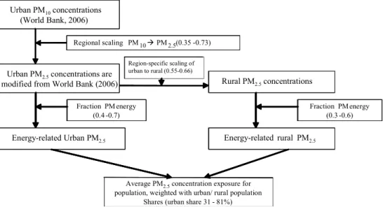
lack the impacts in rural areas. The two approaches were combined by applying scaling factors characteristic for each region, allowing us to derive rural background PM concentrations from urban PM levels. Figure 1 schematically illustrates where these scaling factors are applied, and how, accordingly, the total PM2.5 concentrations from the initial

urban PM10 concentrations are derived per region for the base year 2000.

Figure 1 illustrates both CO2 and PM10 emissions, which allows a study of the potential

synergies between GCC and LAP policies. The WHO PM concentrations have been lowered with another set of scaling factors to obtain values for PM emissions that stem from energy use only. In MERGE a region-specific linear relationship is used between the PM2.5

concentration level G and PM10 emission level H:

5_{As opposed to the WHO (2004), which only measures the number of deaths above a threshold concentration level (7.5 μg/m}3_{), an}

(19)

t,r r

t,r α H

G = , (6)

in which α is the constant expressing this linear relationship: it is region-specific and incorporates the ratio between concentrations of PM10 and PM2.5. Alternatively, this analysis

could have linked PM2.5 concentrations directly to PM2.5 emissions, but proves that the latter

are derived mostly from PM10 emission data inventories anyway.

Figure 1. Flow scheme for the calculation of PM2.5 concentration levels.

As with PM concentrations, in many regions of the world incomplete data are available on the levels of energy-related PM10 emissions. Europe is one of the exceptions, however, as

large databases have been constructed over the past decades to feed the highly publicized policy debate on air pollution. Deliberations resulted in a multi-gas and multi-effect protocol that put stringent limits on the emissions of a series of air pollutants. The results of the integrated assessment of a range of air pollutant abatement options obtained by the RAINS model were important inputs to the public discussions that led to the protocol (Amman et al., 2004a). This model is connected by mapping the technologies simulated in MERGE to the sectors analyzed in RAINS. Table 2 lists energy-related PM10 emissions in the year 2000

taken from a set of different sources as obtained from the RAINS database and transformed for use as input in this extended version of MERGE.

The equations added to MERGE to cover the emissions of PM10, per type of activity p, in

year t, in region r, read:

⎟ ⎠ ⎞ ⎜ ⎝ ⎛ ₋ =

∑

x x,p,t,r p,t,r r t p p,t,r s A q H _,_, 1 , (7) and Urban PM10 concentrations (WHO, 2006) Urban PM2.5 concentrations (modified from WHO (2006)

Regional s caling PM₁₀Æ PM_2.5(0.35 -0.73)

PM2.5 Regional background

Energy related Urban PM2.5 Energy related regional PM2.5 Fraction PM energy

(0.4 -0.7)

Fraction PM energy (0.3 -0.6)

Estimate regi onal PM_2.5: (0.55 -0.68)*C urb

Average PM2.5 concentration exposure for population, weighted with urban/ rural population

Shares (urban share = 31 -81%) Urban PM10concentrations

(World Bank, 2006)

Urban PM2.5concentrations are

modified from World Bank (2006)

Regional scaling PM₁₀Æ PM_2.5(0.35 -0.73)

Rural PM2.5concentrations

Energy-related Urban PM2.5 Energy-related rural PM2.5

Average PM2.5concentration exposure for

population, weighted with urban/ rural population Shares (urban share 31

-Region-specific scaling of urban to rural (0.55-0.66) 81%) Urban PM10 concentrations (WHO, 2006) Urban PM2.5 concentrations (modified from WHO (2006)

Regional s caling PM₁₀Æ PM_2.5(0.35 -0.73)

PM2.5 Regional background

Energy related Urban PM2.5 Energy related regional PM2.5 Fraction PM energy

(0.4 -0.7)

Estimate regi onal PM_2.5: (0.55 -0.68)*C urb

Average PM2.5 concentration exposure for population, weighted with urban/ rural population

Shares (urban share = 31 -81%) Urban PM10concentrations

(World Bank, 2006)

Urban PM2.5concentrations are

modified from World Bank (2006)

Regional scaling PM₁₀Æ PM_2.5(0.35 -0.73)

Rural PM2.5concentrations

Energy-related Urban PM2.5 Energy-related rural PM2.5

Average PM2.5concentration exposure for

population, weighted with urban/ rural population Shares (urban share 31

-Region-specific scaling of urban to rural (0.55-0.66)

(20)

∑

=

p p,t,r

t,r H

H , (8)

in which p is the index referring to elements in the total set of MERGE technologies or activities, the most important ones of which are listed in Table 2. The index, A, measures the level of a specific activity (measured in EJ), where s is the activity-specific emissions factor (measured in Mton/EJ), and 0<q<1 the abatement intensity equal to the marginal (incremental) fraction of emissions reduced per abatement effort index x∈ {1,…,11} from a

specific set of EOP measures (see also equation 9).6 In equation 8 the emissions in year t and

region r are summed over the emissions from all activities. Running MERGE involves choosing the optimal levels for A and abatement q.

Table 2. Energy-related PM10 Emissions (Mt) in 2000 in OECD Europe as modelled in

MERGE based on data from RAINS

RAINS sector MERGE technology Acronym Emissions

of PM10 (Mt)

Coal

Existing power plants Old power plants CR 0.100

Direct use Non-electric applications CN 0.498

Oil

Existing power plants Old power plants OR 0.014

Direct use Transport OT 0.535

Derived products Chemical products ON 0.021

Other

Primary to secondary energy Total primary energy TP 0.131

Total 1.299

N.B. The last entry, primary to secondary energy / total primary energy, refers PM10 emissions from refineries

and transport of energy.

6_{The index x represents a discrete number of steps ranging from {1, …, 11}. Each step is associated with a fixed uniform marginal}

cost level for all activities within a region. As x increases, the uniform fixed cost level increases as well. For example, in Europe at x =1, the marginal cost level is fixed at 379$ / t PM10 (=350 euro / t PM10), at x = 2 this level is fixed at 1623$ / t PM10 (1500 euro / t

PM10), and, finally at x=11, the marginal costs occur above 155,000$ / t PM10 (144,000 euro / t PM10). The 11 steps with fixed

marginal cost levels and the incremental abatement intensities q (% emissons reduction; no dimension) reproduce the Marginal Abatement Cost Curves (MACCs) for Europe based on RAINS.

(21)

There are two additional technology options not mentioned in Table 2 that are optional from 2020 onwards: ‘clean’ coal-fired power stations in the electricity sector and renewables in the transport sector. The former are power plants that produce zero emissions of PM10, but still

emit the usual levels of CO2. An example of the latter concerns bio-diesels for use as

transport fuel, the combustion of which does not generate net emissions of CO2 but does emit

PM10. These two types of technologies play a peculiar role in this model, as they are

acclaimed to be relevant for either GCC or LAP policy, with the characteristic of each of them to be stimulated under one policy, while simultaneously being discredited under the other one.

Which of these two stimuli will dominate cannot be acclaimed a priori, but can only be derived through factual model runs. For the base year, the emission factors s are assumed to be uniform across regions for each activity. Of course, especially for activities in low-income regions, like India and China, assuming the same emission factors seems rather unrealistic. But since calibrated PM10 emissions have been calibrated to actual concentrations of PM2.5

for the year 2000, and the MERGE program is based on a comparison between emission reduction costs and it’s impact on monetized damages through concentration changes, the induced error on optimal mitigation behaviour will likely be smaller than this gross approximation in terms of emissions may suggest. For the reference year 2000, s is defined as the ratio, in Europe, between PM emissions (as in RAINS) and the output of PM-emitting activities (as in MERGE). The emission factors are assumed to decrease over the coming decade, being kept at their 2020 values thereafter. The decline over time of emission factors is based on the baseline scenario downloaded from Internet and also reported in Amman et al. (2004b).7

For the uncertainty analysis on the emission factors of developing countries, SO2 emission

coefficients for Europe (see Amman et al., 2004a) and China (see Foell et al.,1995) are compared. The difference (%) of emission factors of SO2 between these two regions were

used as a proxy for PM emission coefficient differences, and were applied to all developing countries.

2.5 EOP-abatement costs of PM

The alternative to experiencing damages as a result of PM emissions is avoiding them. There are EOP measures that significantly lower energy-related PM10 emissions. The RAINS model

simulates such abatement technologies for Europe and includes data for their costs in each sector. Particularly because abatement options can be ordered according to increasing deployment costs, RAINS adopts distinct Marginal Abatement Cost Curves (MACC’s) for different PM10 emission activities. These MACC’s constitute the graphical representation of

emission reduction costs in each sector for the ranked set of available abatement

(22)

technologies. MERGE does not have any explicit specification of abatement technologies, and basically the same MACC’s are adopted as used in RAINS, after some mapping procedures similar to those already explained. As in RAINS, it is assumed that not all abatement options can immediately enter the market. It takes time to develop abatement technologies, even if the required know-how to implement them is already available. For 2020, the model is only allowed to deploy measures up to 50% of the total feasible reduction potential. For 2030, this threshold is set at 75%, and beyond 2040, the full range of options is implementable. Figure 2 plots the MACC’s for the six main PM-emitting activities in Europe.

As can be seen from Figure 2, the abatement costs remain below 5,000 $/tPM10 for most

activities (except TP) when PM10 emissions are reduced by only 10%. When emission

reduction levels increase to 70%, abatement costs increase to at least 10,000 $/tPM10, but in

most cases they are factors higher. For the short term, the same European MACCs are employed in MERGE as in RAINS for end-of-pipe PM abatement technologies. For the coming years, however, these cost curves are lowered to account for an autonomous reduction in abatement technology costs within a sector. On the other hand, GDP will rise over time, as a result of which the costs of producing abatement technologies will increase, since higher wages will push production costs up. In particular, it is assumed that abatement costs will increase according to this phenomenon at 50% of the GDP growth rate. Both the cost-reducing and cost-incrementing tendencies are simulated in the MERGE model. MACCs similar to those of Figure 2 are applied to all world regions. For this purpose, it is typically the y-axis of the figure that is stretched, so that the same abatement options become cheaper in China, for example, in comparison to those in Europe. For the time dependence of MACCs in other regions similar adjustments are made. A side-effect of this approach is that ‘low-hanging fruit’, as implemented in Europe for the last twenty years or so are excluded as an option in China. This is admittedly a shortcoming. The total PM10 abatement costs K for each

region r and year t as in equation (1) come to:

∑

⎥ ⎦ ⎤ ⎢ ⎣ ⎡ = p x p,t,r x x,p,t,r p,t,r p,t,r t,r s A q Q K _, , (9)

where Q represents the marginal costs associated with reducing PM10 emissions through

end-of-pipe abatement techniques (y-axis of Figure 2), indexed for each activity A and marginal abatement effort index x∈ {1,…,11}, and q the marginal fraction of emissions reduced (this

is not the fraction of emissions reduced as plotted on the x-axis of Figure 2, but the incremental value). As previously mentioned, it is also assumed that PM emissions from the use of renewable energy, , the abatement costs (in absolute terms) of renewables (although emission coefficients are lower than for oil) exceed those of oil (about 33%).

(23)

There is an analogue between PM10-end-of-pipe abatement costs, as added to MERGE, and

the non-CO2 abatement costs, as implemented by Manne and Richels (2004). Manne and

Richels report: ‘For the abatement of non-energy emissions, MERGE is also based on EMF 21. EMF provided estimates of the abatement potential for each gas in each of 11 cost categories in 2010. We incorporated these abatement cost curves directly within the model’. In this modified MERGE model the feedback of EOP expenditures are incorporated through K in equation 1. Manne and Richels continue with ‘abatement cost curves… extrapolated after 2010, following the baseline’ and ‘an allowance is also built in for technical advances in abatement over time.’ The marginal increments in this modified MERGE model are also changed in equation 9. Thus MERGE also allows for a technical change in abatement activities from reduced opportunity costs associated with abatement activities over time.

Recalling from Table 2 that the most dominant sources for PM10 emissions are the OT and

CN activities (almost 90% of Europe’s PM10 emissions), the total abatement costs are also

dominated by end-of-pipe measures related to these activities. For example, the demand for oil can be seen to have a limited abatement potential equal to 20% if the marginal costs remain below 50 US$ per Kg PM10. But the abatement potential can be increased to more

than 90% if the marginal costs are increased to more than 54 US$ per Kg PM10 (smoke filters

on passenger cars).

Figure 2. Marginal abatement cost curves for the six PM10-emitting activities of

Table 2 as adopted from RAINS, as applicable to the year 2000 in Western Europe.

0 25 50 75 100 0 0.2 0.4 0.6 0.8 1

Fraction of emissions reduced

Marg inal ab atemen t co sts (i n 20 00 US$ / k g) CN CR ON OT OR TP

(24)

(25)

3 Results

In order to analyze the effects of GCC and LAP control, three different policy scenarios are defined; the expanded MERGE model was run for each of these. Externalities are internalized in these policy scenarios: in other words external costs (or environmental dual prices) are included in the prices for energy services and consumer goods. In a baseline (business-as-usual) scenario these external costs are set at zero8. For all four scenarios the main findings

are reported in terms of both calculated CO2 emission paths, and the costs and benefits of

policy intervention. The first policy scenario (GCC) internalizes GCC damages: MERGE finds the Pareto-optimal pathways for energy use, considering the total costs and benefits of CO2 emissons reductions in all regions. The second scenario (LAP) internalizes LAP

damages: energy system pathways are calculated on the basis of the full costs and benefits of PM technology implementation. The third scenario (GCC+LAP) internalizes GCC and LAP damages, yielding energy technology implementation paths that account for all costs and benefits of both CO2 and PM reduction efforts.

3.1 CO

2

emissions

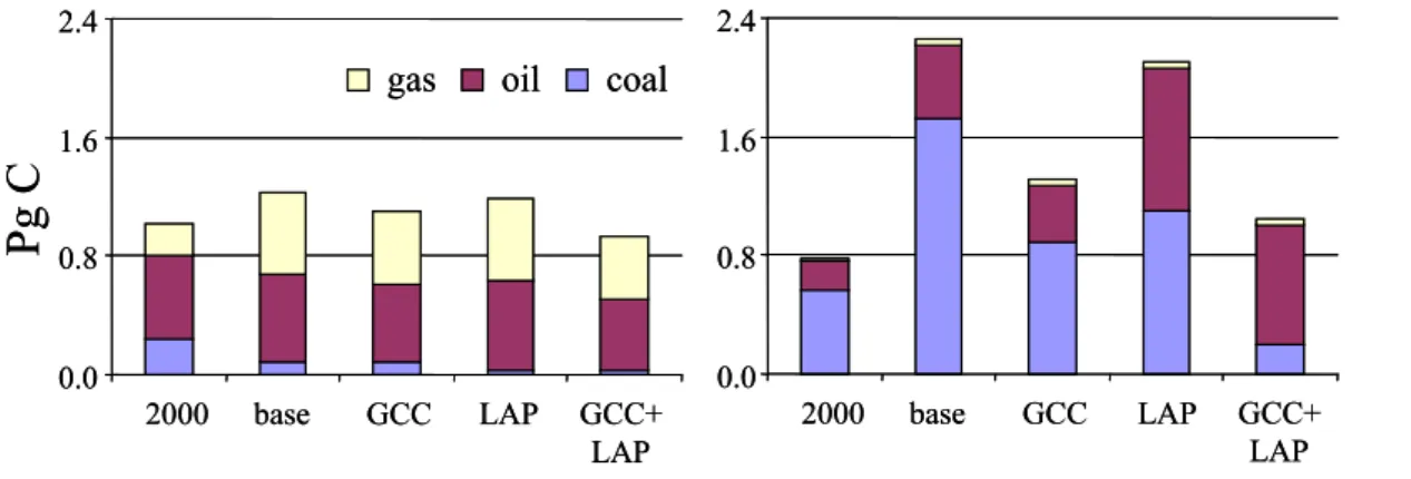
As a result of the internalization of LAP and GCC externalities, the emissions from all sources are subject to change. Figure 3 depicts the total energy-related emissions of CO2

generated by Western Europe and China for the years 2000 and 2050, specified by scenario and differentiated by source of production. For 2050 both the baseline and the three scenario emission levels are shown. A distinction is made between the three fossil fuels, coal, oil and natural gas, as each of them behaves differently under the respective policies investigated. Purposefully, the choice has been made to show the results for Western Europe and China. As for the former, Western Europe constitutes a representative and well-documented reference case (which was the reason that the emission coefficients for all regions were calibrated to West-European data). The latter is particularly important, as China’s future energy use will likely dominate global energy demand and CO2 emissions in the year 2050,

especially under the baseline assumptions. The West-European share to total global energy use (17% today) is assumed to have decreased to 9% by 2050, whereas China’s share (9% in 2000) will have risen to 15% over this period.

As can be seen from Figure 3, CO2 emissions at present are larger in Western Europe than in

China. While emissions in Western Europe over the coming 40 years only slightly increase,

8_{The assumption on the measures included in the MACCs and the evolvement of a costless decline of emission intensities, as}

defined for our baseline scenario, can be argued to be arbitrary. One can also argue that there should be no decline of emission intensities and more measures included in the MACCs. But we think our guesstimate fits best with the assumptions of the IPCC B2 scenario, as currently applied to MERGE simulations (see Nakićenović et al., 2000).

(26)

as shown in the baseline bar of Figure 3, in China the level of these emissions almost triples and thereby will have largely surpassed that of Western Europe in 2050. The main reason is the large difference in prospected economic growth between these two regions. There are also differences between Europe and China in terms of the present and future relative shares of the different sources contributing to total CO2 emissions. The use of coal, for example, plays a

much more prominent role in China than in Western Europe, in all scenarios, while the role of natural gas remains almost negligible in the former. China’s coal use is predominantly expanded in the fields of electricity generation by coal-fired power plants and heat production through the direct combustion of coal. Both these prospected increases in coal usage greatly enhance China’s CO2 emissions. In Western Europe, the use of coal currently contributes

significantly to the emissions of CO2, but its share is expected to decrease sharply over the

coming decades. European use of natural gas, on the other hand, is increasingly becoming more important.

The level and source of emissions are strongly dependent on the scenario simulated, especially for China. Internalizing GCC damages as disutility in consumption (compared to the baseline with the GCC scenario) reduces CO2 emissions in both regions, but mostly in

China. The reason is that China emits much more, while possessing cheaper CO2 abatement

options. The reduction of total CO2 emissions in China is mainly driven by a decrease in the

use of coal, whereas in Western Europe the (more modest) reduction in CO2 emissions results

mostly from a cut in the demand for oil. As can be seen from the global picture in Figure 4, GCC policy only moderately affects the level of PM emissions, in comparison to those in the baseline, both for Western Europe and China.

When LAP policy is applied, on the other hand, more than 90% of global PM emissons reductions are obtained, yet the inclusion of LAP externalities as disutility in consumption has little effect on the level of CO2 emissions. This occurs in both Western Europe and China,

as can be seen from Figure 3. Most of the PM emissions are reduced through the implementation of end-of-pipe abatement measures. For example, it is assumed that all newly installed coal-fired power plants from 2020 onwards use ‘clean coal technology’, that is, they do not generate PM emissions but continue to emit CO2. Since the application of PM

reduction technology under LAP policy is costly, it can be seen that for Western Europe the use of coal and the corresponding CO2 emissions decrease. In China the same can be

observed, while another phenomenon is also at work: a trade-off emerges between different forms of energy. The use of oil instead of coal for heating purposes possesses a PM reduction potential, so that coal is replaced by oil in the LAP scenario for China (see Figure 3). In China, the impact of LAP policies on the origin of CO2 emissions is thus larger than in

Western Europe. Oil was observed to remain a predominant energy source in all scenarios and regions, because there are limited opportunities to reduce oil demand in the transport sector, while its PM emissions can be duly addressed.

(27)

Figure 3. Total energy-related CO2 emissions in Western Europe and China in 2000

and 2050 according to scenario and source of production.

If the GCC and LAP policies are combined, there is little to gain in terms of additional reductions in PM emissions, since LAP policies alone already eliminate most of these emissions. For CO2, however, Figure 3 demonstrates that by combining these policies extra

CO2 emission reductions can be achieved, that is, more than follows from the sum of the

application of either policy alone. By comparing the GCC and GCC+LAP scenarios in Figure 3, the synergy between these policies can be seen: i.e. the simultaneous inclusion of both GCC and LAP externalities results in an additional energy-related CO2 emission

reduction of 15 % in Western Europe and 20 % in China. The explanation is that, by choosing technologies that simultaneously reduce CO2 and PM emissions, one generates cost

savings in EOP abatement that can be utilized to deploy further CO2 abatement options. In

other words, extra CO2 emission reductions become economically feasible that previously

were not. Also, learning dynamics justify higher energy costs for the mid-term (and lower costs for the long term). This process increases the emission abatement efficiency, as it generates supplementary cost decreases and corresponding savings, augments the CO2-free

technologies deployment potential, and thus yields deeper cuts in CO2 emissions, achievable

under the GCC+LAP scenario but not under the GCC or LAP policy case alone.

3.2 Costs and benefits

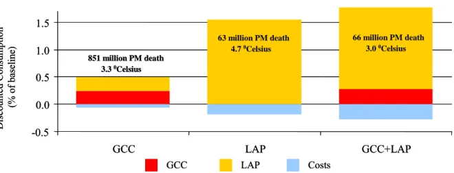
Figure 4 shows the net impact on global welfare, resulting from both costs incurred and benefits obtained, expressed in terms of the percentage change (with respect to the baseline) of the total discounted sum of consumption up to 2150, for each of the three different policy scenarios. For simulating the baseline scenario the GCC loss factor E and the LAP loss term F in equation (2) are set to 1 and 0, respectively. For the GCC and LAP scenarios these parameters are ‘switched on’, to values <1 (E in equation 3) when climate change damages are internalized, and >0 (F in equation 4) when PM air pollution damages are internalized, respectively (while for the GCC+LAP scenario both parameters are switched on). A comparison of the total discounted consumption stream corrected for values of E and F, as

Western Europe China

gas oil coal

Pg

C

0.0 0.8 1.6 2.4 2000 base GCC LAP GCC+ LAP 0.0 0.8 1.6 2.4 2000 base GCC LAP GCC+ LAP

Western Europe China

gas oil coal

Pg

C

0.0 0.8 1.6 2.4 2000 base GCC LAP GCC+ LAP 0.0 0.8 1.6 2.4 2000 base GCC LAP GCC+ LAP

(28)

differences between the baseline, on the one hand, and the respective scenarios, on the other, generates the benefits of GCC and/or LAP policy intervention as reported in Figure 4. The first two bars represent the scenarios, in which the external costs of GCC and LAP, respectively, are separately internalized in the prices of energy services and consumer goods. The third bar denotes the scenario in which both LAP- and GCC-related external costs are simultaneously accounted for. The costs incurred are depicted below the x-axis and the avoided monetary damages (i.e. the benefits) resulting from GCC and/or LAP policy above the x-axis. The benefits are differentiated between those of climate change mitigation (GCC, lower part) and of PM emissions reduction (LAP, upper part). Also indicated for each scenario is the cumulative number of premature deaths due to PM2.5 emissions and the

long-term (2150) equilibrium temperature change with respect to its pre-industrial level as a result of GHG emissions. For the baseline scenario these observables amount to 1083 million and 4.8˚C, respectively, over the period 2000-2150.

Figure 4. Changes in costs, benefits, and global welfare for three scenarios (GCC, LAP, and GCC + LAP), expressed as percentage consumption change in comparison to the baseline.

A first and important finding from Figure 4 is that GCC policy (first bar) delivers benefits, not only for GCC but also for LAP, while purely LAP-oriented policy (second bar) only brings forward LAP benefits. Figure 4 also demonstrates that in all three scenarios the benefits gained from environmental policies (leading to reductions in CO2 and PM10

emissions) largely outweigh the costs of these policies (inducing a reallocation of financial resources to implement end-of-pipe abatement measures). The first bar shows that internalizing GCC externalities in MERGE yields a clear net improvement in global welfare. It proves, however, that there are not only large (expected) benefits in terms of GCC, but also (unexpectedly) approximately equal benefits in terms of LAP. The reason is that newly

Di sc ou nt ed Co ns um pt io n (% of ba se lin e) GCC LAP Costs -0.5 0.0 0.5 1.0 1.5 GCC LAP GCC+LAP 63 million PM death 4.7 0_Celsius 66 million PM death 3.0 0_Celsius 851 million PM death 3.3 0_Celsius Di sc ou nt ed Co ns um pt io n (% of ba se lin e) GCC LAP Costs -0.5 0.0 0.5 1.0 1.5 GCC LAP GCC+LAP 63 million PM death 4.7 0_Celsius 66 million PM death 3.0 0_Celsius 851 million PM death 3.3 0_Celsius

(29)

installed technologies such as renewables and CCS not only contribute to reducing CO2

emissions but also decrease those of PM.9

The second bar shows that internalizing LAP damages yields a net global welfare improvement that is even significantly larger than in the first case. Moreover, internalizing LAP damages in MERGE is found to lead to an optimal solution with environmental benefits at the global level as a result of PM emissions abatement that outweigh the climate benefits as calculated with the original MERGE model by a factor of approximately 5. However, the GCC benefits obtained in the LAP scenario amount to zero.10 The first reason is that LAP

reduction is mainly achieved through the installation of EOP technologies which strongly abate the emissions of PM, but which only slightly reduce the CO2 emissions. Secondly, it

proves that a switch in fuel-mix by the deployment of renewables, or a change in the nature of energy supply by the application of CCS technologies to fossil-fired power plants (both as means to reduce PM emissions) only materialize in the long term, i.e. after 2040.11 As a result,

their significance in controlling the change in global atmospheric temperature, and thus the corresponding climate change mitigation benefits, remain only relatively small. In addition, it proves that many of the CO2 emissons reductions realized are partly offset by an expansion of

the aforementioned clean-coal technologies. These are coal-based technologies that are retrofitted with PM-abatement techniques (and as such receive an impetus from LAP policy, as they are generally cost-competitive), but still remain potent CO2 emitters. The impulse

given to such clean-coal technologies is a perverse effect of LAP policy, as they are counter-productive for climate change control. Thus, overall the LAP scenario does little to reduce the global level CO2 emissions, and does not generate any climate change benefits in terms of

improvements to welfare.

The third bar in Figure 4 shows that there are synergies to be obtained from simultaneously internalizing LAP and GCC externalities in the production of energy and goods. As demonstrated in this figure, the costs and benefits of the GCC+LAP scenario are not merely the sum of those of the individual GCC and LAP scenarios. The total costs of the third scenario (GCC + LAP) are slightly larger than the sum of the costs of the individual GCC and LAP scenarios. But the total benefits of the third scenario are greater than the combination of those in the GCC and LAP policies, and the corresponding increase is larger than the increase in costs incurred, thus implying an overall net welfare gain. Note that the LAP benefits do not increase by going from the LAP to the GCC+LAP scenario, since a reduction is kept in

9_{The installation of CCS technologies is assumed to achieve a reduction in PM emissions.}

10_{Although there are no monetized GCC benefits, there will be a reduction in the temperature level of 0.1˚C due to moderate CO}

2

emissons reductions. The policies to avoid LAP improve welfare, and at given temperature levels, the willingness to avoid climate change will increase as a result of improvement in welfare. Thus policies may yield physical benefits of avoided damages that do not result in monetary gains.

11_{Note that these renewables are mostly non-biomass in nature, as, for example, the production and use of ethanol derived from}

(30)

premature deaths from 1083 down to 66 million cumulated. The GCC benefits, however, clearly increase, as the stabilization temperature becomes 3.0˚C in the GCC+LAP scenario, rather than 3.3˚C in the GCC scenario. This ‘bonus’ is obtained through the long-term time perspective of MERGE, in which a synergy between GCC and LAP policies can be created through a gradual transition of the energy system to one in which ‘double-clean’ technological options are deployed, i.e. that serve GCC mitigation and LAP reduction at once. The assumptions in MERGE on the way future cost reductions are achieved for both new options like renewables and retrofit-ones like end-of-pipe abatement applications are instrumental here. Note that the results presented in Figure 4 are driven mainly by changes taking place in developing countries, as these are assumed to dominate the global economy in the long term.

(31)

4 Uncertainty analysis

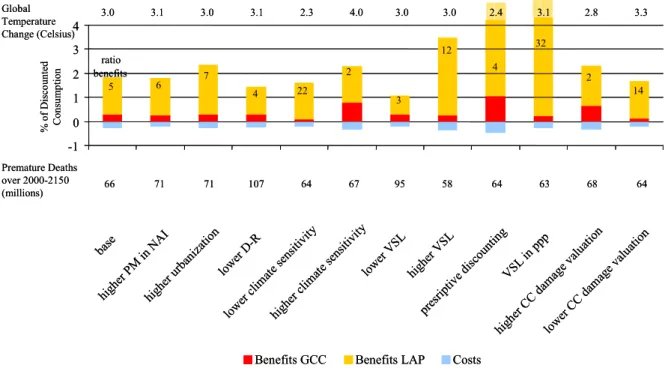
A model like MERGE allows for calculating and comparing the optimal time-dependent GHG and PM emission pathways, both globally and per region, for the impacts of these substances under different assumptions. In its cost–benefit mode, MERGE can generate monetary values for the corresponding environmental benefits of climate change mitigation and air pollution reduction. The results, however, are subject to a range of specific parameter assumptions, especially those related to impacts. Figure 5 presents the results of a detailed uncertainty analysis for the most relevant of these assumptions in terms of the globally aggregated discounted costs and benefits of the implemented policies. The base case is the same as the GCC+LAP scenario specified in Figure 4. Costs (the bars below the 0-line) and benefits (the bars above the 0-line, differentiated into GCC and LAP benefits) are expressed as the percentage change of total discounted consumption, for each of the different parameter variations. The numbers shown in the upper bars refer to the ratio of LAP to GCC benefits obtained. As indicated in the first bar for the base case, for example, this ratio is about 5. The numbers above the figure are the calculated global mean temperature changes (3˚C in the base case) and those below the figure are the premature deaths from 2000 to 2150 (66 million in the base case). All respective sensitivity variations are clarified in more detail under the headings I-VIII below.

Figure 5. Sensitivity of GCC and LAP policy costs and benefits, expressed as relative change of total consumption for a range of important parameter variations.

Global Temperature Change (Celsius) Premature Deaths over 2000-2150 (millions) % o f Di sco unt ed Consum pt io n base higher PM in NAI higher u rban ization lower D-R lowe r clim ate se nsitivit y higher c limate sensitivi ty lower VS L highe r VS L pres riptiv e disc ountin g VSL in ppp

higher CC dam age v aluation lower CC da mag e valu ation

Benefits GCC Benefits LAP Costs

3.0 3.1 3.0 3.1 2.3 4.0 3.0 3.0 3.1 2.8 3.3 66 71 71 107 64 67 95 58 64 63 68 64 -1 0 1 2 3 4 ratio benefits 5 6 7 4 22 2 3 12 4 32 2 14 2.4 Global Temperature Change (Celsius) Premature Deaths over 2000-2150 (millions) % o f Di sco unt ed Consum pt io n base higher PM in NAI higher u rban ization lower D-R lowe r clim ate se nsitivit y higher c limate sensitivi ty lower VS L highe r VS L pres riptiv e disc ountin g VSL in ppp

higher CC dam age v aluation lower CC da mag e valu ation

Benefits GCC Benefits LAP Costs

3.0 3.1 3.0 3.1 2.3 4.0 3.0 3.0 3.1 2.8 3.3 66 71 71 107 64 67 95 58 64 63 68 64 -1 0 1 2 3 4 ratio benefits 5 6 7 4 22 2 3 12 4 32 2 14 2.4

(32)

I. Higher LAP emissions in developing regions

PM emission coefficients and abatement cost curves for all regions are derived from European data. Given the lack of appropriate data in many parts of the world, this is currently the best possible approach, even though the PM emission coefficients of developing countries are likely to be underestimated. This is because the calibration does not reflect the changes over the past few decades in Europe’s PM10 emissions through the implementation of

EOP-abatement technologies. Related to this is the fact that in developing countries today there are likely to be cheaper abatement options available to lower present emissions of PM. To account for the observation that developing countries might have undertaken less stringent abatement activities and thus could be faced with lower marginal costs, a joint sensitivity check was performed: the energy-related PM emission coefficients for non-Annex I (NAI) regions are increased by a factor of 4 (based on an analogous comparison between SO2

emission intensities: see Foell et al., 1995, and Amman et al., 2004a). In parallel it is assumed that the marginal costs of PM abatement activity of the first 75% of a given emission level can, for example, in China be reduced at the lowest possible costs. The lowest possible costs are equal to the lowest marginal costs of the MACC’s that apply in the base case. Finally, α (see equation 6) is lowered by factor of 4 to simulate the same base-year concentration level of the benchmark case. The marginal cost of abatement of the remaining 25% of the abatement potential equals the cost curve of the base case. As a result of these combined changes, the total costs of global PM abatement efforts decrease, while their environmental benefits increase, and thus the LAP-GCC benefit ratio augments to 6 (see the second column of Figure 5).

II. Higher urbanization assumptions in developing countries

In the baseline it is assumed that with a growing world population, the ratio between the number of people living in urban versus rural areas remains constant. Especially in developing regions, however, people tend to migrate towards cities and densely inhabited areas. Since PM is mostly emitted in urban areas, the total population in these regions will, consequently, be more exposed to it. LAP regulation is thus also likely to generate more benefits. A gradually increasing level of urbanization is modelled by letting α in equation (6) rise over time, implying higher PM2.5 concentration levels for given emission levels, an

indirect way of saying that more people are exposed to a fixed value of the PM2.5

concentration. The value of α is assumed to increase by 0.5% per yr, up to a level of 40% higher than in the base case. The third column of Figure 5 shows that the corresponding higher urbanization assumptions increase the ratio of LAP versus GCC benefits to 7. The effectiveness of LAP policy increases as a result of larger achievable long-term health benefits.

(33)

III. PM emissions-concentration relationship

What if the linear relationship between PM10 emissions and PM2.5 concentrations of equation

(6) proves to be a square root instead? This would mean that the effect of emission abatement to concentration reductions of PM2.5 is currently overestimated. End-of-pipe PM10 emissions

abatement efforts in reality thus preclude fewer premature deaths than currently assumed. The dose-response (D-R) relationship of equation (6) adapted for the corresponding sensitivity exercise (involving an adjusted set of values for the parameter α to achieve the same concentration levels as in the base year of the benchmark case) leads to the fourth column of Figure 5. Indeed, the benefits obtained from LAP policy decline, and the ratio of LAP to GCC benefits decreases to 4. Given the reduced efficacy of LAP policy, the number of premature deaths increases significantly.

IV. Lower and higher climate sensitivity

One of the most speculative parameters in analyzing GCC is the climate sensitivity, referring to the long-term global average temperature increase corresponding to a doubling in the atmospheric concentration of CO2 with respect to pre-industrial levels. Under a given climate

change control target, this parameter is among the main determinants for the pervasiveness of CO2 emission reduction levels (see, for example, van der Zwaan and Gerlagh, 2006). In the

base case, the climate sensitivity is fixed at a 2.5˚C. If the climate sensitivity is lower (higher), the damages incurred by CO2 emissions will be lower (higher), and thus will call for

less (more) climate mitigation efforts, and correspondingly yield less (more) benefits of GCC policy. Given the observed link between LAP and GCC policy, lower benefits of GCC policy involve, likewise, somewhat lower benefits of the LAP policy. The climate sensitivity values investigated by us are 1.5˚C (low case) and 4˚C (high case), resulting in a decrease, respectively increase, of the benefits of GCC policy, as demonstrated by the fifth and sixth columns of Figure 5. The corresponding ratio of LAP versus GCC benefits moves up to 22, respectively down to 2. In the high climate sensitivity variant, resulting in the lower bound for all LAP-GCC benefit ratios derived from the multiple sensitivity exercises, this ratio is still well above 1.

V. Lower and higher VSL

Assumptions regarding VSL are the key to cost–benefit analyses. In CAFE, a VSL of 1.06 million US$ is assumed as the base case (Holland et al., 2005). This source reports a VOLY of 57,300 US$, which is multiplied by the presumed value of 10 for YOLL as a result of chronic exposure to PM2.5 in Europe (Pope et al., 2002).5 For the VSL sensitivity exercise,

the resulting VOLY-based figure is adopted as the lower bound. The upper bound is 2.1 million US$, corresponding to the estimate for VSL in the USA (US-EPA, 1999).12

12_{Actually, this ‘environmental’ VSL equals one-third of the total VSL. Here the same rule is adopted as applied in Holland et al.}

Local air pollution and global climate change: a combined cost-benefit analysis

Abstract

Rapport in het kort

Contents

1

Introduction

2

Methodology