PBL WORKING PAPER 16 JANUARY 2014 Modelling housing preferences using decision tables: method and empirical illustration
MANON VAN MIDDELKOOPa and HARRY BOUMEESTERb
a PBL Netherlands Environmental Assessment Agency, P.O. Box 30314, 2500 GH The Hague, The Netherlands
b OTB - Research for the Built Environment, P.O. Box 5030, 2600 GA Delft, The Netherlands
Contact manon.vanmiddelkoop@pbl.nl and h.j.f.m.boumeester@tudelft.nl
Abstract
Quantitative theories and approaches have been dominant in a variety of disciplines. In this contribution, we will explore an alternative approach: decision tables, i.c. sets of decision rules extracted from an existing data set using a CHAID-based algorithm, that focus on conditions and states leading to particular actions or decisions. These decision tables make for an attractive approach in the context of rule-based (parts of) microsimulation models of consumer choice behaviour. The approach is illustrated by modelling people's preferences in choosing a new dwelling. In addition, the flexibility of the approach is used to demonstrate how the characteristic of 'housing affordability' is related to both the desired dwelling and the potential buyer or tenant. Rules are extracted from data on stated preferences, collected in the Netherlands in 2009.
JEL classifications C44, R21, D12 and C63
Keywords Housing preferences – Decision tables – Decision rules - Rule-induction algorithm – CHAID
1.
Introduction
To support and evaluate housing policies and marketing strategies, many theories and models of preference and choice have been advanced to assess the evaluation of housing options by households. Already in the mid-1990s, Witlox (1995) introduced Decision Tables (DTs) in housing research as an attractive alternative to more quantitative approaches and as a superior alternative to the use of decision rules in Decision Plan Nets (DPNs). After that, it fell silent around DTs in housing research. This paper therefore re-introduces DTs to housing research and demonstrates its potential in the context of assessing housing preferences of moving inclined households.
From the 1970s onwards, cognitive-behavioural (choice) models have been advanced to quantify and test the functional relationship between the characteristics of decision makers (e.g. age, household composition) and dwelling features (e.g., tenure, surroundings), preferences for (composite) housing choice alternatives, and the probability that an alternative will be selected (Timmermans and Golledge, 1990). Once a model has been estimated and validated, alternative scenarios and policy measures can be evaluated by expressing the changes in terms of the condition variables. Using the estimated relationships, the most likely behaviour under the assumption of time-invariant behaviour is predicted.
Basically, existing choice models can be classified into two groups of models. Utility-maximising models, assume individuals do always select the (set of) alternative(s) that maximises their total utility (Ben-Akiva and Lerman, 1985). Like other classical approaches advocating economic decision makers to maximise their profit, these models assume decision makers to possess complete knowledge of all relevant information and to act completely rational in their pursuit of maximum utility. Utility-maximising models focus on one or more dwelling features. Given the characteristics of the decision maker, they try to quantify the contributions of the identified features to the overall utility of these dwellings. The method of measuring housing preferences or (hypothetical) choice can be attribute-based (compositional) or alternative-based (decompositional). Decompositional approaches evaluate dwelling profiles as a whole, and statistical methods are applied to estimate the contributions of attributes and attribute levels. Conjoint Analysis is a good example of this approach (Molin, 2011). Compositional methods explore housing preferences by recording separately and explicitly how people evaluate housing attributes. Using some algebraic rule, the importance of each attribute can be weighted and combined to arrive at an overall evaluation. Multi-attribute Utility Technique (MAUT) is one of these methods (Jansen, 2011).
The concepts of preference and choice are widely used in housing research, often related to the stage of the lifecycle and the context of the housing market. Preference, as an expression of attractiveness, may guide choice, but the evaluation involved in preference may take place whether or not a choice has to be made. The most important difference between housing preference and housing choice, is that preference is a relatively unconstrained evaluation of attractiveness. Although several studies have suggested that tenure preferences are adjusted, at least to a
certain extent, to individual and contextual factors that may hamper moving into homeownership (e.g. see De Groot et al., 2013; McLaverty and Yip, 1993) In the case of a house, choice will always reflect the joint influences of preference, market conditions, regulations, and availability.
Despite the popularity of utility-maximising models, it has been argued that the theory of utility maximisation may not represent individual decision-making very accurately. In line with comments on rational choice theory, advocates of non-utility-based models, the second group of behavioural choice models, argue that people may not always behave rational. It is, for instance, not realistic to assume full-information required for utility-maximising choice behaviour. Another element of criticism on utility-maximising models (and other approaches based on (neo-)classical economic principles), challenges the idea that people are free to choose the alternative that matches their preferences best. Decision makers also have to take into account, for instance, their (social) environment (coupling constraints; Hägerstrand 1970). Also, the field of behavioural economics coming into vogue in the 1980s, provided several new concepts to explain departures of (economic) decision making from neo-classical theory. Most notably Kahneman and Tversky’s (1979) prospect theory, forwarding the idea that people make decisions based on the potential value of losses and gains rather than the (utility of the) final outcome, and that people evaluate these losses and gains using certain heuristics. Decision making under risk is then described using concepts such as loss aversion, anchoring (reference dependence), non-linear probability weighting and context dependency such as insolation effects and certainty effects (Kahneman and Lovallo, 1993).
Taking these arguments together, it is not realistic to assume decision makers to possess adequate knowledge and willingness to evaluate the utility of each alternative in the choice set, identify the alternative that gives the highest utility, and then select that alternative. Although utility-based time and money allocation models assume individuals to be constrained by financial and temporal budgets, there are many more sources of constraints (Hägerstrand, 1970). Based on modern psychological and physiological theory, various alternative theories and modelling approaches have been advanced that aim to imitate human decision making processes in the brain. The development of non-utility-based models, is often conceptualised as a problem of training a system based on examples, i.e. observed or stated housing preferences. In many cases, heuristics or decision rules are used to describe the relationship between the decision maker and context and the decision itself. Decision rules reflect experience-based techniques for problem solving, learning, and discovery and include both desires and constraints of decision makers. They are represented by logical expressions (e.g., IF <condition state(s)> THEN <action>).
In contrast to quantitative utility-based approaches, rule-based models are more qualitative. As a consequence, the latter approaches offer more flexibility in modelling housing choice behaviour because they do not assume an a priori functional form. Nor do they require variables to follow a particular distribution. In addition, both compensatory and non-compensatory decision rules can be included, and decision rules are able to account for a high degree of interpersonal variation – in particular when probabilistic rules are used. This potential higher flexibility in
representing alternative decision processes of qualitative models, does not necessarily imply that they are better predictors of observed choice behaviour than conventional quantitative models. However, several studies in shopping location choices (Thill and Wheeler, 2000), daily activity scheduling and transport (Arentze et al., 2000, Wets et al., 2000) and tourist choices (Van Middelkoop et al., 2000) indicate that rule-based models at least match the results of conventional utility-based models. In short, rule-utility-based model are theoretically ahead, offer more flexibility and at the very least come up to the performance of utility-based models. Inspired by this assessment and the application in other fields, this article re-introduces the use of decision tables to housing research. In particular, we propose to model the preferences for a new dwelling of moving inclined households by describing the propensity to select each relevant dwelling feature by a probabilistic decision table (DT; i.c. a set of decision rules). Subsequently, a composite overall propensity or preference probability of a household for a dwelling is obtained by multiplying the probabilities for each separate dwelling feature.
This contribution is organised as follows. First, we will provide a background on housing preferences and choices. Next, we will discuss the principles underlying DTs and the algorithm that is used to extract decision tables from empirical data. Finally, we will illustrate the approach in the context of housing preferences.
2.
Lifecycle theory and housing choice
People’s acting and thinking are often based on a long-term vision in order to provide continuity and security in life. Current behaviour is adapted according to a person’s long-term preferences. The individual endeavours to give his/her life shape according to fairly consistent paths, are denoted as careers. People can follow parallel, strongly connected careers for different areas of their lives, such as education, work, leisure, creating a household and living (Clark and Dieleman, 1996; Mulder, 1993; Mulder and Hooimeijer, 1995; Priemus, 1984).
Life-long studies have shown that there is a clear connection between events in these careers and moving house (Aarland and Nordvik, 2009; van Ham, 2002; Harts and Hingstman, 1986; Kim et al., 2005). An event in a particular career often triggers a desire to move house. This career is denoted as the triggering career. The other careers are, in this situation, seen as the conditioning careers which help to determine the possibilities and restrictions to the search (Boumeester, 2004; Feijten and Mulder, 2002; Goetgeluk, 1997; Karsten, 2007; Mulder, 1993).
Changes in the household cycle or work cycle lead to changes in the housing needs of households. If the current housing situation deviates too much from the altered needs, this can lead to moves to another dwelling and living environment. It is assumed that the dwelling and the living environment are made up of a collection of features or attributes. People in different stages of the lifecycle will therefore ascribe different values to these attributes. They have a preference for those attributes to which they ascribe greater value. An idea of the ‘popularity’ of a particular dwelling can be obtained by considering all part-values together, often using some algebraic rule. The popularity of a dwelling appears thus to vary between households with different dwelling needs and positions in the job market. The same
dwelling can have a completely different value for one household than for another. A dwelling can also have different total values for the same household over time, if the household itself enters a different stage of the lifecycle.
Working out the preference structure is central to this research. Sometimes ‘revealed preference’ research is used to study that structure, assuming that the choice is a good reflection of a person’s preferences. This will only be the case if the consumer can make the most optimal choice on the housing market with sufficient supply. However, in a tight market where people probably have to deal with second best or less optimal housing supply, the actual choice is not a good reflection of the preference (Groot et al., 2013). In that case, studying the preferences using a ‘stated preferences’ approach is preferred.
Three choices are made in the course of the decision to move into a particular dwelling or housing unit, each choice inextricably tied to the other two. In general, the choice of the timing of a move, the tenure choice and the choice of the level of housing services are made simultaneous, because they are interrelated (Elsinga, 1995; Laakso and Loikkanen, 1992). In the Netherlands, for instance, the choice for a bigger apartment or for a single-family dwelling is easier to achieve in the owner-occupied sector then in the rental sector (Boumeester, 1996; Clark et al., 1994; Oskamp, 1997). And if a household wants to move to an affordable dwelling in the short-term, the owner-occupied sector again gives more opportunities. If the desired type of dwelling (tenure, location or level of housing services) is not available, a household can choose to postpone (or cancel) the move. If postponing is not possible, the household has to substitute the desired characteristics of the dwelling (Dieleman and Everaers, 1994; Laakso and Loikkanen, 1992; Oskamp, 1997)
In the Dutch context, some overall patterns can be found between the position in the life cycle and the position on the labour market on the one hand and housing choices on the other. These ‘housing careers’ are influenced by the housing culture and governmental policy on tax reduction and housing allowances. These policies often steer households in the higher income groups into the owner occupied sector because that is financially preferable. Comparable households with a lower income are in general better off by renting a dwelling for financial reasons. At the start of the housing career, younger households more often live in the rental sector, in smaller dwellings and in apartments. When household size or income increase in later years, larger single-family dwellings and the owner-occupied sector become more desirable. By aging, the household size and income often decrease, and households that are inclined to move start looking again for smaller houses, houses in the rental sector and apartments. (Boumeester, 2004; Elsinga 1995; Ministry of the Interior and Kingdom Relations and CBS, 2013; Mulder, 1993).
However, the actual moving behaviour also depends on the constraints imposed by the housing market (Dieleman and Everaers, 1994; Meen, 1998; Mulder and Hooimeijer, 1995). The availability and accessibility of the preferred dwelling are involved (Fitzpatrick and Pawson, 2007). The primary supply of rental and owner-occupied dwellings as the starting point of house-moving chains also plays a role. The secondary supply (dwellings which become available through the filtering of households), is in volume even more important, especially for starters on the housing market who often select their first home from the existing stock.
In many countries, people do not normally save up to buy a home (Boumeester, 2009; Elsinga, 1995). It is the availability of mortgages that largely determines the accessibility of owner-occupied dwellings. This accessibility is, in addition to the level of household income, strongly determined by mortgage interest rates, the types of mortgage on offer, the criteria applied with respect to the loan-to-income (and initial loan-to-value) ratio, the collateral value of the dwelling and (national) tax regulations. Additionally, for owner-occupiers, the equity in the current dwelling (or, given the recent drop in housing prices: the lack thereof) is also an important factor. Beside the income of a household, wealth in a broader sense determines the choice of desired tenure and the level of housing services for rental dwelling (Abraham and Hendershott, 1996; Boelhouwer, 2005; Boumeester, 2009; Meen, 1998; Megbolugbe and Linneman, 1993).
3.
Decision rules and tables
Decision rules are not new to housing research, on the contrary. Decision Plan Nets (DPNs) based on a step-by-step interviewing techniques, for instance, represent the decision rules an individual uses in a tree-structured diagram. Its application has proven to be quite useful in housing research (see, for example, Goetgeluk, 1997; Goetgeluk and Hooimeijer, 2002; Op 't Veld et al., 1992; Oskamp 1997; Witlox 1995, 1998). However, DPNs also have a number of important limitations (see Witlox (1995) for an extensive discussion). First, the validity and reliability of the DNP method have been questioned. This revolves around the question whether respondents are capable of accurately articulating a DPN that truly reflects their decision making process. Second, individual DNPs are very difficult to aggregate and the method also lacks an explicit error theory to allow for measurement errors and omitted variables. Third, DPNs only allow for binary evaluations of decision criteria. Fourth and finally, attributes in a DPN may spread through the whole decision net structure and exhibit changing dimensions.
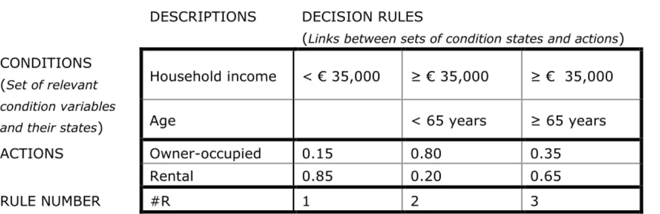
Already in the mid-1990s, Witlox (1995) introduced Decision Tables (DTs) as a superior alternative to DPNs in housing research. A DT is a matrix-like representation of the decision making process that consists of condition variables (left upper part), their levels or states (right upper part), actions or decisions (left bottom part) and rules that link condition states to actions (right bottom part; Mors, 1993;Verhelst, 1980; see figure 1). Rules can both be crisp, where all cases complying with the specified conditions are assigned to the most likely choice alternative (deterministic all-or-nothing assignment). Or rules can be more fuzzy or probabilistic, where cases are assigned to the available choice alternatives with a certain probability (probabilistic assignment).
The easiest way to understand a DT is to read one. Figure 1 presents a (fictive) three-rule DT describing the preferences of households for tenure types. Start with the first question (condition): What is the household income? If the answer (condition state) is lower than 35,000 euros, rule number 1 states that 15 percent of the households prefer an owner-occupied dwelling and 85 percent prefer a rental dwelling (action). If the answer is at least 35,000 euros, the preference for owner-occupied dwellings increases (rule numbers 2 and 3). In this case, the tenure
preference further depends on the age of the head of the household: up to 80 percent of households under 65 years prefer an owner-occupied dwelling (rule 2), whereas only 35 percent of the older higher-income households are interested in the owner-occupied segment of the housing market (rule 3)
DESCRIPTIONS DECISION RULES
(Links between sets of condition states and actions) CONDITIONS
(Set of relevant condition variables and their states)
Household income < € 35,000 ≥ € 35,000 ≥ € 35,000
Age < 65 years ≥ 65 years
ACTIONS Owner-occupied 0.15 0.80 0.35
Rental 0.85 0.20 0.65
RULE NUMBER #R 1 2 3
Figure 1 Demonstrative example of a decision table: the (fictive) preference for the tenure type of a dwelling given two characteristics of the moving inclined household
DTs offer a more compact, efficient and effective visual presentation, ease of manipulation and ability to check information on consistency, exclusiveness and exhaustiveness. This is due to the strict format. Consistency means that for each possible combination of condition states, it should be unmistakable which actions should be performed. Exclusivity implies that at least one element of the condition part in a decision rule does not intersect with the corresponding element in the condition part of another rule. Exhaustivity, finally, means that every condition state of each condition variable is included in the rulebase, and that for each combination of condition values an action is specified.
Originally a technique used to support programming, DTs were gradually introduced to different domains, knowledge representation and decision support systems in particular (Moreno Garcia et al., 2000). The application of DTs was greatly stimulated with the introduction of algorithms building decision tree-structures from empirical data, for then it became possible to extract consistent, exclusive and exhaustive DTs from stated or observed choices and preferences1.
4.
Induction of rules
Several algorithms from both information theory and statistics build decision tree-structures from empirical data, and subsequently transform this tree into a set of
1 In the original application of DTs, unlike decision trees, the condition variables used for splitting have a fixed and identical order across the decision rules. In our application, DTs are induced from a secondary data set using tree-induction algorithms. The condition variables used for splitting do not have a fixed or identical order, nor does the DT necessarily become as compact as its original counterpart. The tree-based algorithm does, however, provide for the three properties that together guarantee the evaluation of every possible decision making context (defined by the available condition variables).
rules. In the context of housing choices, these tree-induction systems use condition variables (that is, characteristics of the decision-making household and context) to repeatedly partition the sample of housing choices or preferences into mutually exclusive and exhaustive sets of conditions states that are more homogeneous with regard to the housing choices or preferences. In figure 1, for instance, income is the most important condition variable (out of a set of condition variables) with regard to tenure preferences. And, within the higher income segment, age is the next most predictive variable to further split the population. By considering splits (and mergers) as the only permissible operations, tree-building algorithms guarantee that the sets of decision rules are exclusive, exhaustive and consistent; applying the resulting DTs to other cases will always assign each new case unassailably to one action (decision), and one action only.
Many different criteria can be defined for selecting the best (combination of) condition states to split up the population with regard to the decision under consideration. Stopping criteria often include significance or improvement testing of possible combinations of condition states and/or the specification of a minimum number of observations within each (set of) condition states before or after split. The sets of observed housing choices are thus defined by combinations of - or interactions between - condition states (Magidson, 1995; Strambi and Van de Bilt, 1998). By linking the response distribution of a set of observed housing choices or preferences defined by a particular set of condition states to the actions, a decision rule is obtained. Hence, in the rule-based framework, the decision rule reflects the probability that a comparable household under similar conditions would select or prefer a particular dwelling feature.
The most commonly applied tree-building algorithms are C4.5, CART and CHAID. For practical reasons, such as the widespread use and knowledge of the
2 -test and the availability in SPSS, and theoretical considerations such as the greater sensitivity to the whole response distribution (which is favourable in the light of probabilistic decision rules), we use CHAID2. It is acknowledged, however, that this comes at the cost of more elaborate sets of decision rules and that, given the present state of knowledge regarding the application of rule-induction systems in the social sciences, the choice in favour of any algorithm is at least in part arbitrary (Van Middelkoop et al., 2000; Wets et al. 2000).5.
Chi-Squared Automatic Interaction Detection (CHAID)
Like any other tree-building algorithm, CHAID (Kass, 1980) recursively splits a sample of choice observations on condition variables. It uses
2-statistics, including user-defined significance-testing levels, and user-defined minimum numbers of observations, to reach the maximum level of homogeneity within decision rules with2
The CHAID-algorithm was originally introduced as an exploratory technique (Kass, 1980), but it has also been used for prediction, classification/segmentation, as well as for detection of interaction between variables. Today, it is often used in the context of direct marketing to select groups of consumers and predict how their responses to some variables affect other variables. Clark, Dieleman and Deurloo introduced CHAID to housing research in the early 1990s (see, for example, Clark and Dieleman, 1996; Clark et al., 1990).
regard to the decision (in our case: preference) under consideration. The algorithm starts by initialising a decision table with a single column, representing a decision rule. The frequency distribution of respondents across the choice alternatives then represents the heterogeneity of responses in the total sample. In order to maximize the reduction of this heterogeneity while at the same minimizing the number of splits (decision rules), the CHAID-based algorithm then computes the
2-statistics and corresponding “pairwise” p-values for each pair of the condition states that is eligible to be merged. If the largest of all pairwise p-values is greater than a user-specified -level, this pair of states is merged into a single compound condition state, and the whole process is repeated (with this new compound state) until the largest pairwise p-value at a certain stage is smaller than the user-specified
-level. The merging process is repeated for each condition variable and its states in turn.Next, for each optimally merged condition variable, the (adjusted) p-value of the (reduced) decision table is computed. If there has been no reduction of the original table, a
2-test can be used that is conditional on the number of categories of the condition variable. However, if the table has been reduced, a more conservative significance test should be used to avoid the risk of capitalising on chance in search for the optimal grouping of condition states. In the CHAID-based algorithm, the adjusted p-value is obtained by using a proper Bonferonni multiplier. Basically, this multiplier is determined by the number of ways a condition variable of a given type with c original condition states can be reduced to r states (1 ≤ r ≤ c; Kass, 1980).Given the adjusted p-values of all conditions, the condition variable with the lowest p-value is isolated. In statistical terms, this variable is the most significant predictor with regard to the choice or preference under consideration. If the p-value of this condition variable is smaller than or equal to the specified
-level, the group of observations is split according to the (merged) states of this condition variable. If no condition variable has a significant p-value, the (sub)population is not split, and the process is terminated. For each partition of the data that has not been analysed, the algorithm returns to the first step. The tree-growing process continues until all subgroups have either been analysed or contain too few observations.6.
Illustration
6.1 Definition of the problem
Within a regional microsimulation model of the housing market, households and dwellings are the main units of interest. Both types of units have certain characteristics such as age, income and composition as indicators of the status of various household careers and tenure type, size, location and price in the case of dwellings (see also the section on lifecycle theory). The most interesting feature of any housing market model, however, is the link between these units, since each household resides in a specific dwelling at a specific location. In due course, households may wish to adjust their residential situation and start looking for a dwelling that better matches their preferences. In order to support the simulation of this process, a microsimulation model requires a module describing the housing
preferences of these moving inclined household. Which household has a higher probability of valuing which dwelling most, given the status of the other careers, the present housing situation and the features of the dwellings on offer? Or, stated differently, who is most likely to move to which dwelling?
In a microsimulation model under construction, this process is modelled using several stages that parallel those in real housing market choice processes. First, the model has to ‘decide’ which households will become inclined to move given the characteristics of both the household and the present dwelling (this stage is not covered in this paper). Next, the model has to establish a link between the moving inclined households and the primary and secondary supply of dwellings. Both households and dwellings are characterised by several features (based on lifecycle and housing choice theories described in section 2 and data availability). Decision rules derived from the expressed housing preferences of moving inclined households are used to model the probability that a certain household in a certain choice context will prefer a certain dwelling feature (see hereafter). The probability that a particular moving inclined household will prefer a certain dwelling (characterised by multiple features) is obtained by multiplying the probabilities for preferring individual dwelling features. The latter operation is valid since DTs for dwelling features are induced conditional on higher order dwelling features (recall that housing features in the Netherlands are seriously intertwined). By definition, the sum of all preference probabilities for all possible dwellings (that is, all possible combinations of all dwelling features) for one household equals 1. Using a multiplicative function, implicitly a non-compensatory preference structure is assumed where a low preference probability on one attribute can hardly be compensated for (Jansen et al., 2011). Alternatively, if there are strong indications for compensatory preference structures, a linear additive function should be used.
Next, the matching process clears the market in several rounds representing a one year cycle. The simulation model is able to imitate both tight and ‘buyers-’ market situations. In tight market situations, where households would have to ‘fight’ to obtain a dwelling, a set of several households is ‘offered’ to a vacant dwelling. Using the induced DTs, the probabilities that these households would prefer the features of this dwelling are calculated based on the features of the households and the dwelling. These part-values are combined to obtain an overall probability that a household will prefer this particular dwelling. Finally, the household with the highest probability is selected (alternatively, using a Monte Carlo approach, the calculated preference probabilities can be used to select a household with a certain probability). The selected household then ‘moves’ to this new dwelling, while the home that is available for the market is included in the next round as part of the secondary supply (save dwellings that are to be demolished). Households that, after a certain number of ‘fights’ do not have obtained a dwelling, have to reconsider their initial housing preferences by releasing their ambitions with regard to one or more dwelling features (including location) or, alternatively, become ‘non-moving-inclined’ again. The latter substitution or postponement process is not covered in this paper.
In contrast, the ‘buyers’ market’-situation currently present in the owner-occupied sector, can be mimicked by ‘offering’ a set of available dwellings to one moving inclined household which, subsequently, selects the one with the highest
probability score (above a certain threshold level, and/or with a certain probability – if so desired).
As argued before, we have chosen a rule-based approach, using a CHAID-based algorithm to induce decision rules for the preferred dwelling features from empirical data. The induction of the DTs and their validation and interpretation are not discussed here. This would require many pages since the induced DTs include up to 307 decision rules. A brief impression of the most important decision conditions for each DT is provided in box ‘A sketch of the induced DTs’. Instead, the focus of this paper lies on calculating and discussing the composed preferences of eight example households for five show dwellings using two different sets of DTs to illustrate the application of DTs within the context of a microsimulation model. The two sets of DTs differ with regard to the conceptualisation of the relative costs of a dwelling: is it a characteristic of the household (i.e. a condition variable) or a dwelling feature (i.e. an action variable)? First, however, the next subsection outlines some important data issues.
6.2 Data and example households and dwellings
Secondary analysis on the Netherlands Housing Survey 2009 dataset (WoonOnderzoek Nederland 2009) is used. This survey-based study aims to compile statistical information from households on past and current housing preferences and housing costs using computer-assisted personal, telephone and web interviewing. The sample consists of 78,000 Dutch residents aged 18 and over, who do not reside in institutions or shelters. The survey was conducted between September 2008 and April 2009, with 1 January 2009 serving as the data survey date (Ministry of VROM and CBS 2010; National Government, 2013). We use data on 21,660 moving inclined respondents representing 2 million moving inclined households (weight factor with an average ‘blow-up’-factor of 93.2) to induce DTs describing the desirability of dwelling features.
Tree-based algorithms like CHAID require large amounts of cases. Although there are no strict guidelines, a minimum sample size of 1,000 records is often used (Thorn, 2008). To reduce the risk of over-fitting – a DT might fit the initial data well, but perform poorly on other populations – the minimum sample sizes are set at 100 records before, and 45 records after performing splits that define the condition states (see Van Middelkoop (2001) for experiments with stopping criteria). Since respondents are weighted to represent all moving inclined households in the Netherlands, the stopping-criteria for the CHAID-based algorithm are blown-up with the average ‘blow-up’-factor of 93.2; i.c. the stopping criteria are set at 9,320 households before and 4,194 households after a possible split. For the same reason, the user-specified -level, is set rather conservatively at 0.01.
The Netherlands Housing Survey 2009 only identifies the preferences of moving inclined households for individual dwelling features. Trade-off or substitution dimensions are not registered. This raises some important questions. For instance, does the questionnaire lure respondents into expressing unrealistic housing preferences? E.g. the proverbial “villa in Amsterdam” for the price of a social rented apartment in some peripheral area? De Jong et al. (2008: 126-128) show expressed
housing preferences to differ between regions, indicating respondents to be well aware of supply constraints3. De Groot et al. (2013: 469) conclude that regional differentiations in house price-to-rent ratio have influence already on the formation of the preference to move into homeownership. Also, an additional survey on the NHS 2009 shows that moving inclined households who actually did move, barely substitute on tenure, type of dwelling and price (Ministry of the Interior and Kingdom Relations, 2011). De Groot et al. (2013: 477) shows that only 13% of the aspiring homeowners moved to a rental dwelling while 56 percent did not move at all. A longitudinal study in the Netherlands over the period 2002-2005 shows that 8 percent of the moving inclined households with a preference to rent end up in the owner occupied sector (Das and De Groot, 2012). Due to the nature of the data, the overall preference of a moving inclined household for a specific dwelling can only be obtained by combining preferences for individual dwelling features. By ‘simply’ multiplying the probabilities that households will prefer certain dwelling features to obtain an overall preference for a dwelling, dwelling features are implicitly assumed to have similar weights. According to Jansen (2011) this is more or less the case for the main preferred features of the dwelling. Next, the overall preference of various households for one dwelling can be compared4, and the dwelling can be allocated to the household with the highest overall preference. This mirrors the situation in a tight housing market. Alternatively, the overall preferences of one household for several dwellings can be compared to imitate the choice process in a more relaxed housing market.
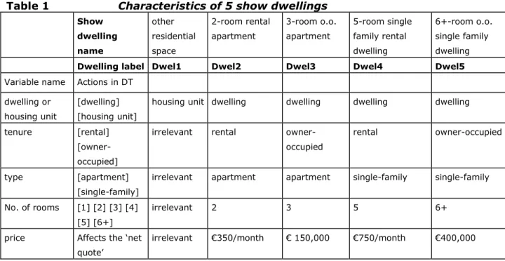
In order to illustrate the application of DTs in a microsimulation model, preferences of eight sample households for five show dwellings are calculated. Five features characterize the show dwellings (see table 1). The preferences for each dwelling feature (except for price; see hereafter) are described using DTs. Since dwelling features are severely intertwined, a sequential approach is adopted, where preferences for lower order dwelling features are induced for each higher order feature separately. The preferences for single-family dwellings vs. apartments, for instance, are induced for (would-be) owner-occupiers and tenants separately.
3 In some cases, we found would-be home-buyers to express ‘desired’ purchase prices that do not seem realistic in relation to their (gross) income and available equity in and outside the current home and given the 2009 Code of conduct regarding mortgage loans (Dutch: Gedragscode Hypothecaire Financieringen). This makes sense, if one considers that some respondents have only come up with the idea of moving house rather shortly before being interviewed, and have not gathered much information yet (while others will already have a more realistic picture of their possibilities). In these cases, we adjusted the ‘desired purchase price’ and the resulting ’aspired’ interest quote to meet the regulations in force. This adjustment picks up a lead on the substitution (or adjustment) process that is included in the simulation model in later stages.
4 Remember that the decision rules reflect the probability that a similar household under similar conditions will prefer a particular dwelling feature, where the sum of the probabilities for the actions (dwelling feature categories) within one decision rule sum up to one. Hence, the preferences for all theoretically possible dwellings (i.e. all combinations of all dwelling feature categories) of a household sum up to one too, and the preference for a particular dwelling (i.e. the product of the probabilities that a household will prefer the individual dwelling features) hence reflect the attractiveness of a particular dwelling on a scale from 0 to 1.
Table 1 Characteristics of 5 show dwellings Show dwelling name other residential space 2-room rental apartment 3-room o.o. apartment 5-room single family rental dwelling 6+-room o.o. single family dwelling
Dwelling label Dwel1 Dwel2 Dwel3 Dwel4 Dwel5
Variable name Actions in DT dwelling or
housing unit
[dwelling] [housing unit]
housing unit dwelling dwelling dwelling dwelling tenure [rental]
[owner-occupied]
irrelevant rental owner-occupied
rental owner-occupied
type [apartment]
[single-family]
irrelevant apartment apartment single-family single-family No. of rooms [1] [2] [3] [4]
[5] [6+]
irrelevant 2 3 5 6+
price Affects the ‘net quote’
irrelevant €350/month € 150,000 €750/month €400,000
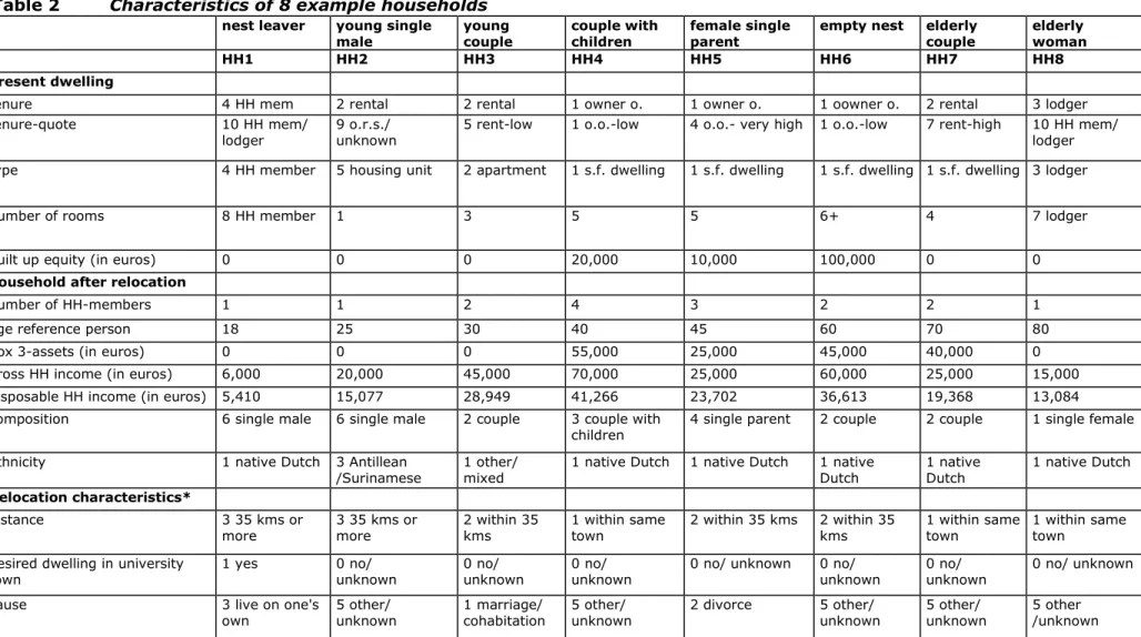
The eight example households typically illustrate the demographic life cycle and range from a nest leaver to an aged widow. Their characteristics are shown in table 2 and include the features of the present dwelling, socio-economic characteristics of the household after it has moved house and information on the desired relocation itself. Except for the disposable household income, these characteristics were fed into the CHAID-based algorithm as condition variables to induce the decision rules for the consecutive dwelling features. In order to make the microsimulation model sensitive to changes in housing and tax regulations, the net amount of euros that is spent on a dwelling relative to the disposable income of the household is used as an indicator of the costs rather than the actual monthly rent or the selling/purchase price. This ‘net interest or rent quote’ (‘quote’ hereafter) is not available in the Netherlands Housing Survey 2009 dataset, but is constructed based on the available data. This calculation is based on information on:
- the desired dwelling price as expressed by the moving inclined respondent: desired monthly rent or purchase price
- characteristics of the moving inclined household: disposable and gross income and possible assets and equity in and outside the present dwelling that can be used to lower the mortgage loan of the next home (these variables underestimate the actual income and assets for single person households who are going to cohabit after the move)
- the statutory regulations, agreements and laws (in force in 2009) with regard to housing and income tax: including housing allowance for low income renters, tax deductions and additions for owner-occupants, buyer’s costs and the guidelines banks used in 2009 to assess the maximum mortgage loan (see footnote 3)
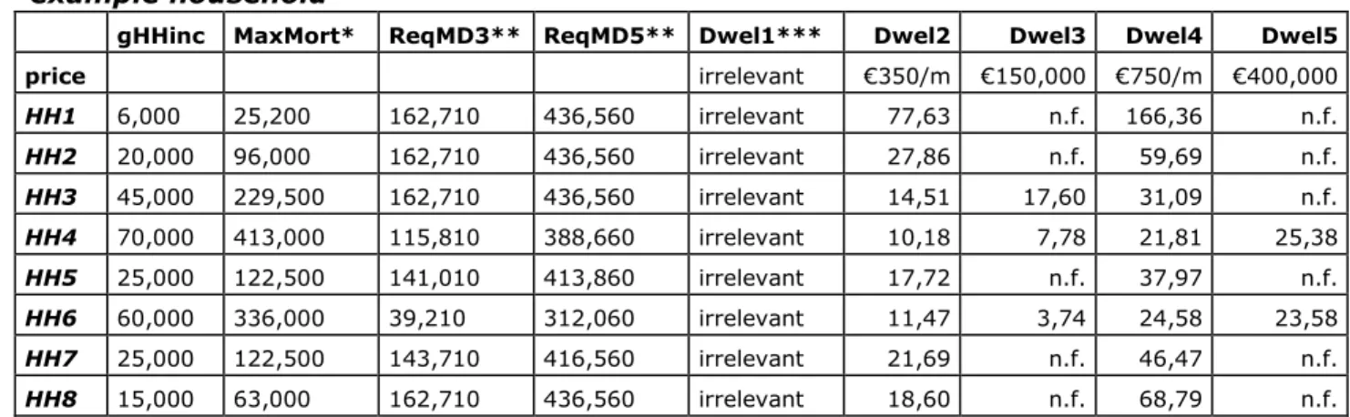
The quotes for the dwelling-household combination considered in this paper are presented in table 3.
Table 2 Characteristics of 8 example households
nest leaver young single
male young couple couple with children female single parent empty nest elderly couple elderly woman
HH1 HH2 HH3 HH4 HH5 HH6 HH7 HH8
present dwelling
tenure 4 HH mem 2 rental 2 rental 1 owner o. 1 owner o. 1 oowner o. 2 rental 3 lodger
tenure-quote 10 HH mem/
lodger 9 o.r.s./ unknown 5 rent-low 1 o.o.-low 4 o.o.- very high 1 o.o.-low 7 rent-high 10 HH mem/ lodger type 4 HH member 5 housing unit 2 apartment 1 s.f. dwelling 1 s.f. dwelling 1 s.f. dwelling 1 s.f. dwelling 3 lodger
number of rooms 8 HH member 1 3 5 5 6+ 4 7 lodger
built up equity (in euros) 0 0 0 20,000 10,000 100,000 0 0
household after relocation
number of HH-members 1 1 2 4 3 2 2 1
age reference person 18 25 30 40 45 60 70 80
box 3-assets (in euros) 0 0 0 55,000 25,000 45,000 40,000 0
gross HH income (in euros) 6,000 20,000 45,000 70,000 25,000 60,000 25,000 15,000
disposable HH income (in euros) 5,410 15,077 28,949 41,266 23,702 36,613 19,368 13,084
composition 6 single male 6 single male 2 couple 3 couple with
children 4 single parent 2 couple 2 couple 1 single female
ethnicity 1 native Dutch 3 Antillean
/Surinamese 1 other/ mixed 1 native Dutch 1 native Dutch 1 native Dutch 1 native Dutch 1 native Dutch
Relocation characteristics*
distance 3 35 kms or
more 3 35 kms or more 2 within 35 kms 1 within same town 2 within 35 kms 2 within 35 kms 1 within same town 1 within same town desired dwelling in university
town 1 yes 0 no/ unknown 0 no/ unknown 0 no/ unknown 0 no/ unknown 0 no/ unknown 0 no/ unknown 0 no/ unknown
cause 3 live on one's
own 5 other/ unknown 1 marriage/ cohabitation 5 other/ unknown 2 divorce 5 other/ unknown 5 other/ unknown 5 other /unknown * In order to (largely) exclude the effect of differences between regional housing markets in this illustration, the desired province for the future dwelling is ‘8 North-Holland’ for all example households.
Table 3 Net interest and rent quotes for each show dwelling, per example household
gHHinc MaxMort* ReqMD3** ReqMD5** Dwel1*** Dwel2 Dwel3 Dwel4 Dwel5
price irrelevant €350/m €150,000 €750/m €400,000 HH1 6,000 25,200 162,710 436,560 irrelevant 77,63 n.f. 166,36 n.f. HH2 20,000 96,000 162,710 436,560 irrelevant 27,86 n.f. 59,69 n.f. HH3 45,000 229,500 162,710 436,560 irrelevant 14,51 17,60 31,09 n.f. HH4 70,000 413,000 115,810 388,660 irrelevant 10,18 7,78 21,81 25,38 HH5 25,000 122,500 141,010 413,860 irrelevant 17,72 n.f. 37,97 n.f. HH6 60,000 336,000 39,210 312,060 irrelevant 11,47 3,74 24,58 23,58 HH7 25,000 122,500 143,710 416,560 irrelevant 21,69 n.f. 46,47 n.f. HH8 15,000 63,000 162,710 436,560 irrelevant 18,60 n.f. 68,79 n.f.
* MaxMort = Maximum mortgage loan according to the Gedragscode Hypothecaire Financieringen (Code of conduct regarding mortgage loans) given the gross household income (gHHinc) and an interest rate of <= 5 %
** ReqMDx = Reguired mortgage for dwelling x, calculated as: 1.02 * ((1.07 * Dwelling price) – Surplus value of the present dwelling) - 0.5 * ‘box 3-assets’; this formula takes into account the expenses to be paid for by buyers (conveyance tax and costs), the costs of mortgage approval and - when relevant - assumes households to invest 100% of the equity build up in the previous house and 50% of the so-called 'box 3'-assets into the new dwelling.
*** Dwelling 1 is a housing unit and the preferences for other features of these units (price/quote, tenure type, number of rooms) are not taken into consideration.
n.f. = not feasible given the required and maximum mortgage
Theoretically, the quote is both related to the desired dwelling and to the potential buyer or tenant. We therefore decided to induce two sets of DTs and compare the results. In the first set, the quote is considered a feature of a dwelling, i.c. the ‘aspired quote’ is a dependent or action variable. In this set, the first DT describes the preferences for the combined tenure-quote choice (since the quotes for tenants differ significantly from those of owner occupants). The combined tenure-quote action variable comprises eight categories: (1) owner-occupant dwelling with a quote below 10.1%; (2) owner-occupant dwelling, quote between 10.1 and 16.4%; (3) owner-occupant dwelling, quote between 16.4 and 20.3%; (4) owner-occupant dwelling, quote of at least 20.3%; (5) rented dwelling, quote below 13.7%; (6) rented dwelling, quote between 13.7 and 20.0%; (7) rented dwelling, quote between 20.0 and 27.7%; and (8) rented dwelling, quote of at least 27.7%. The cut-off values for the quotes were determined by creating four equal-frequency categories of (would-be) owner-occupants and tenants respectively. The next eight DTs determine the preferences for the dwelling type – single-family dwelling or apartment – for each of these tenure-quote groups. The final eight DTs in this set determine the preferences for the number of rooms (1, 2, 3, 4 , 5, or 6+) for each the tenure-quote group (splitting up these groups according to the desired dwelling type would have violated the demand for a minimum sample size of 1,000 records).
In the second set of DTs, the quote is considered a characteristic of the moving inclined household, i.c. the ‘aspired quote’ is fed into the CHAID-algorithm as
a continuous condition variable. In this set, the first DT comprises rules describing tenure preferences. Next, two DTs describe the preferences for the dwelling type of owner-occupants and renters respectively. Finally, four DTs describe the decision rules used by each combined group of (would-be) tenure and dwelling type residents for the number of rooms. Both sets of DTs are preceded by a DT containing the decision rules for aspiring either a dwelling or a housing unit (such as a house boat or a home for the elderly or a student hall). The features of the latter category are not investigated further due to the low number of households aspiring these units. A sketch of the induced DTs
The first DTs describes the conditions that describe the distribution of preferences of moving inclined households for either a dwelling or a housing unit in 237 decision rules. The most important condition variables are household type (where single males and females show a higher preference for housing units), especially when they are young (< 25-35 years) or old (> 55-65 years), as age is often the second most important condition variable.
First set of DTs (combined tenure-quote choice as action variable)
The decision between eight tenure (rental or owner-occupied) and net rent or interest quote situations (low, intermediate, high or very high) is dominated by income: the higher the income, the more households are inclined to buy a house (with the high income also leading to lower interest quotes), while lower income households often express an interest in rental homes, with, as a result of the same income, high rent quotes. The second conditional variable (within various income ranges) may include the present tenure situation and/or net rent or interest quote, but also the desired residential province.
In the subsequent 16 DTs describing the conditions that indicate the preferences for single or multi-family houses and the number of rooms (conditional on the preference for one of the 8 combined tenure-quote choice options), either the number of households members or the household type is the main condition.
Second set of DTs (net interest or rent quote as a condition variable)
In this set, the first DT describes the choice between a rental or an owner-occupied home. In this DTs, the main condition for each of the 268 rules, is the present tenure situation, where, in general, a preference for continuity in tenure situation is expressed. The second condition variable is, for all rules, the ‘aspired’ interest or rent quote. This underlines the consistency between the desired tenure situation and the interest or rent quote and income levels in the Netherlands today. Within the two DTs for the desired dwelling type (conditional on the tenure), household type dominates the preference for either single or multi-family houses. The number of household members, on the other hand, conditions the preferences for the number of rooms (conditional on the preference for a single or multifamily house in either the rental or the owner-occupied sector).
6.3 Results
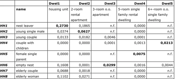
Table 4 presents the composed preferences for each dwelling using the first set of DTs, where the combined tenure-quote variable comprises the first action variable (or dwelling feature). The probability that a household will prefer the first show
dwelling is exclusively based on the DT describing the choice between dwellings and housing units. In a tight market, where the eight households would ‘fight’ for this single living space, the regional microsimulation model for the Dutch housing market would allocate this housing unit to household 1 (marked in bold), since this nest leaver has by far the highest preference for this unit.
The preferences for the other four dwellings are calculated by multiplying the probabilities that the households will prefer each dwelling feature (including the preference for living in a dwelling or a housing unit). The composed preference of the young single male (household 2) for the two-room rental apartment (dwelling 2), for instance, came about as follows: preference of this household for a dwelling (0.963) * preference for a rental dwelling with – for this household – a very high net rent quote (0.341) * preference for an apartment (0.646) * preference for two rooms (0.296) = 0.0627. In a tight market, this apartment would be allocated to the young single male; the three-room owner-occupant apartment (dwelling 3) to the empty nest household (6); the five-room single family rental dwelling (4) to the female single family household (5); and the spacious single family dwelling (5), finally, would be bought by the couple with children (household 4). In a more relaxed market, where there are multiple instances of each dwelling available, the microsimulation model would select the dwelling with the highest composed preference for each household. Evidently, mixes of the assignment rules for tight and relaxed markets are also possible, as would be the use or threshold values.
Table 4 Preference for each show dwelling of each sample household using the first set of decision tables (combined tenure-quote choice as action variable)
Dwel1 Dwel2 Dwel3 Dwel4 Dwel5
name housing unit 2-room
rental apartment 3-room o.o. apartment 5-room single family rental dwelling 6+-room o.o. single family dwelling HH1 nest leaver 0,2730 0,1865 n.f. 0,0000 n.f.
HH2 young single male 0,0374 0,0627 n.f. 0,0000 n.f.
HH3 young couple 0,0133 0,0182 0,0046 0,0001 n.f. HH4 couple with children 0,0000 0,0000 0,0001 0,0013 0,0213 HH5 female single parent 0,0000 0,0000 n.f. 0,0075 n.f. HH6 empty nest 0,1608 0,0001 0,0299 0,0016 0,0044 HH7 elderly couple 0,0688 0,0018 n.f. 0,0000 n.f. HH8 elderly woman 0,1102 0,0271 n.f. 0,0000 n.f.
# computed as the product of the preferences for the following dwelling characteristics: ‘dwelling or housing unit’ * ‘combined tenure-quote choice’ * ‘dwelling type’ * ‘number of rooms’
n.f. = not feasible given the required and maximum mortgage (see table 3)
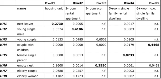
Table 5 shows the preferences of each household for each dwelling using the second set of DTs, where the aspired quotes show up as condition states in the DTs.
Comparing these results to those in table 4, it can be concluded that, in a tight market, the microsimulation model would assign the same dwellings to the same households (again marked in bold). The absolute values of the ‘winning’ preferences, are, however, more pronounced than in table 4, probably due to the lower number of dwelling feature categories. However, the absolute values of the preferences are not as meaningful as the relative differences between the composed preferences within one set of DTs. The choice for either set of DTs should always be based on theoretical or practical arguments relating to the research question under consideration (in this case, be fitted with the objectives of the microsimulation model).
Table 5 Preference for each show dwelling of each sample household using the second set of decision tables (net interest or rent quote as a condition variable)
Dwel1 Dwel2 Dwel3 Dwel4 Dwel5
name housing unit 2-room
rental apartment 3-room o.o. apartment 5-room single family rental dwelling 6+-room o.o. single family dwelling HH1 nest leaver 0,2730 0,2005 n.f. 0,0017 n.f. HH2 young single male 0,0374 0,4106 n.f. 0,0003 n.f. HH3 young couple 0,0133 0,0485 0,0505 0,0105 n.f. HH4 couple with children 0,0000 0,0000 0,0000 0,0179 0,4468 HH5 female single parent 0,0000 0,0013 n.f. 0,0233 n.f. HH6 empty nest 0,1608 0,0014 0,2550 0,0061 0,0458 HH7 elderly couple 0,0688 0,0257 n.f. 0,0003 n.f. HH8 elderly woman 0,1102 0,1723 n.f. 0,0002 n.f.
# computed as the product of the preferences for the following dwelling characteristics: ‘dwelling or not’ * ‘tenure choice’ * ‘dwelling type’ * ‘number of rooms’
n.f. = not feasible given the required and maximum mortgage (see table 3)
7.
Conclusion and discussion
This contribution (re-)introduces qualitative Decision Tables (DTs) induced from a secondary data set as an alternative to the algebraic quantitative theories and approaches that are common to housing research and other domains of consumer choice. DTs and other rule-based models offer several advantages, but also have some drawbacks (see, for instance, Arentze and Timmermans, 2003; Van Middelkoop et al., 2000; Wets et al., 2000; Witlox, 1995). The disadvantages include the fact that the interpretation of the decision rules is not always straightforward as the decision rules do not explain the observed preferences, but merely link them to a particular decision making context. In addition, and unlike the original DTs, DTs
induced by tree-induction algorithms can become quite large. The DT representation format, on the other hand, provides a more compact and efficient representation of the set of decision rules than the decision tree formalism. Due to the discrete nature of condition states, small differences in the decision-making context can bring about substantial and sometimes even counterintuitive shifts in the predictions. In addition, the influence of any particular condition on ultimate choice behaviour is not readily evident and elasticities can only be derived from computing-intensive simulation series.
These (potential) drawbacks come, however, at the prospect of several rewards. First and foremost, qualitative approaches offer much more flexibility in specifying the relationship between conditions and actions and do not impose rigid assumptions on the distribution of variables. Second, DTs offer information on conditional choices with regard to the behaviour under investigation. Which particular method is to be favoured cannot be based on the methodological superiority of one method over another. Rather, the type of information in which one is interested (Hooimeijer, 1994), the desired outcome measure (utility or other) or the source of the preferences (stated or revealed; Jansen et al., 2011) should direct the selection. Third, unlike utility-based approaches such as MAUD (Jansen, 2011) or Conjoint Analysis (Molin, 2011) or another rule-based approach like DPN, DTs using a CHAID-based induction algorithm do not necessarily require a labour intensive and costly data collection process since it allows for secondary analysis of existing data. Fourth and finally, as we have demonstrated, the results of DTs can be combined in several ways to obtain composite measures.
In conclusion, we would like to touch upon some avenues of further research with regard to the latter two advantages. In our empirical illustration we have produced composite probabilities for dwelling preferences by ‘bluntly’ multiplying the probabilities that a household will prefer the individual features. Evidently, introducing more or other features allows researchers to easily transfer the approach to other contexts. In our illustration, for example, we explored some options for the theoretically ambiguous net rent or interest quote. Also, relative weights between the features can be introduces to refine the composite preference structures. Unlike MAUD or Conjoint Analysis, however, these relative weights are not produced by the CHAID-based approach itself, nor can they be obtained from the Netherlands Housing Survey data set. In this context, Magidson and Vermunt (2004) have introduced an interesting extension to the CHAID-based algorithm. They propose a hybrid methodology combining features of CHAID and Latent Class Modeling to build a DT that is predictive of multiple criteria. In our case, for instance, of multiple dwelling features. Future work on this relatively new extension to the CHAID-based analysis would be worthwhile.
Acknowledgements
We would like to express our gratitude for the assistance and suggestions given by our (former) colleagues Andries de Jong, Rob Loke and Carola de Groot (PBL), Gust Marien, Cor Lamain and Roland Goetgeluk (OTB) and the challenging comments raised by three reviewers and the editorial staff of the PBL Working Paper Series that have helped us to improve our work.
References
Aarland K, Nordvik V, 2009, “On the Path to Homeownership: Money, Family Composition and Low-income Households” Housing Studies 24 81–101
Abraham J.M., Hendershott P H, 1996, “Bubbles in Metropolitan Housing Markets” Journal of Housing Research 7 191-207
Arentze T, Hofman F, van Mourik H, Timmermans H & Wets G, 2000, “Using Decision Tree Induction Systems for Modelling Space-Time Behaviour” Geographical Analysis 32 52-72
Arentze T, Hofman F, Timmermans H, 2001, “Deriving Rules from Activity Diary Data: A Learning Algorithm and Results of Computer Experiments” Journal of Geographical Systems 3 325-346
Arentze, T, Timmermans H, 2003, "Measuring Impacts of Condition Variables in Rule-Based Models of Space-Time Choice Behavior: Method and Empirical Illustration" Geografical Analysis 35 24-45
Ben-Akiva M, Lerman S R, 1985, Discrete Choice Analysis. Theory and Application to Travel Demand (The MIT Press, London)
Boumeester H, 1996, “The choice for expensive owner-occupancy in the Netherlands” Netherlands Journal of Housing and the Built Environment 11 253-273
Boumeester H, 2004, Duurdere koopwoning en wooncarrière. Een modelmatige analyse van de vraagontwikkeling aan de bovenkant van de Nederlandse koopwoningmarkt [in Dutch], Thesis (Delft University Press, Delft)
Boumeester H, 2009, “Labour market emancipation results in booming Dutch owner-occupied housing market” in Changing Housing Markets: Integration and Segmentation Eds. M Lux, L Sýkora, O Poláková (The Institute of Sociology of the Academy of Sciences of the Czech Republic, University of Economics, Prague) pp. 1-17
Clark W, Deurloo M, Dieleman F, 1990, “Household Characteristics and Tenure Choice in the U.S. Housing Market” Neth. J. of Housing and Environmental Research 5 251-270.
Clark W, Deurloo M, Dieleman F, 1994, “Tenure Changes in the context of micro-level family and macro-micro-level economic shifts” Urban Studies 31 137-154 Clark W, Dieleman F, 1996, Households and housing: Choice and Outcomes in the
Housing Market (Centre for Urban Policy Research, New Brunswick)
De Jong, A, van den Broek L, Declerck S, Klaver S, Vernooij F, 2008, Regionale woningmarktgebieden: verschillen en overeenkomsten [in Dutch] The Hague/Rotterdam: Ruimtelijk Planbureau/NAi Uitgevers
Dieleman F, Everaers P, 1994, “From renting to owning: life course and housing market circumstances” Housing Studies 9 11-25
Elsinga M, 1995, Een eigen huis voor een smalle beurs: het ideaal voor bewoner en overheid? [in Dutch] Thesis (Delftse Universitaire Pers, Delft)
Feijten P, Mulder C, 2002, “The timing of housholds events and housing events in the Netherlands: a longitudinal Perspective” Housing Studies 17 773-792
Fitzpatrick S, Pawson H, 2007, “Welfare Safety Net or Tenure choice? The dilemma facing social housing policy in England” Housing Studies 22 163–182
thesis [in Dutch] (KNAG/Univeristeit Utrecht)
Goetgeluk R, Hooimeijer P, 2002, The evaluation of Decision Plan Nets for bridging the gap between the ideal dwelling and the accepted dwelling », Cybergeo : European Journal of Geography [on line], Systèmes, Modélisation, Géostatistiques, document 226, mis en ligne le 10 octobre 2002, accessed 24
July 2013. URL : http://cybergeo.revues.org/2379 ; DOI :
10.4000/cybergeo.2379
Groot, C. de, D. Manting, C.H. Mulder, 2013, Longitudinal analysis of the formation and realization of prferences to move into ownership in the Netherlands, Journal of Housing and the Built Environment, 28, 469-488.
Hägerstrand T, 1970, “What About People in Regional Science?” Papers of the Regional Science Association XXIV 7-21
Harts J, Hingstman L, 1986, Verhuizen op een rij: een analyse van individuele verhuisgeschiedenissen [in Dutch], Thesis (Geografisch instituut RUU, Utrecht)
Hooimeijer P, 1994, “Hoe meet je woonwensen?” in Bewonerspreferenties: Richtsnoer voor investeringen in nieuwbouw en de woningvoorraad [in Dutch] eds I Smid, H Priemus. (Delftse Universitaire Pers, Delft) pp. 3-12
Jansen, S.J.T., 2011, The Multi-attribute Utility Method, In: Jansen S, Coolen H, Goetgeluk R (eds.), 2011, The Measurement and Analysis of Housing Preferences and Choice (Spinger)
Jansen S, Coolen H, Goetgeluk R (eds.), 2011, The Measurement and Analysis of Housing Preferences and Choice (Spinger)
Kahneman D, Tversky A, 1979, "Prospect Theory: An Analysis of Decision under Risk". Econometrica (The Econometric Society) 47 (2) 263–291
Kahneman, D, Lovallo, D,1993, "Timid choices and bold forecasts: A cognitive perspective on risk-taking". Management Science 39: 17–31.
Karsten L, 2007, “Housing as a way of life: Towards an understanding of middle-class families’preferences for an urban residential location” Housing Studies 22 83–98.
Kass G V,1980, “An Exploratory Technique for Investigating Large Quantities of Categorical Data” Applied Statistics, 29 119-127
Kendig H, 1984, “Housing careers, life cycle and residential mobility: Implications for the housing market” Urban Studies 21 271-283
Kim T, Horner M, Marans R, 2005, “Life Cycle and Environmental Factors in Selecting Residential and Job Locations” Housing Studies 20 457–473
Laakso S, Loikkanen H, 1992, “Finnish homes; through passages or traps? An empirical study of residential mobility and housing choice” conference paper (International Research Conference: European Cities, Growth and Decline, The Hague)
Magidson J, Vermunt J K, 2004, "An Extension of the CHAID Tree-based Segmentation Algorithm to Multiple Dependent Variables", in Classification - the Ubiquitous Challenge. Procedings of the 28th Annual Conference of the Gesellschaft für Klassifikation e.V., eds. C Weihs, W Gaul (Springer-Verlag, Berlin Heidelberg New York) pp. 176-183