Analysis of Dynamic Node Deployment for UAV-Mounted Base Stations

(1)

UAV-Mounted Mobile Base Stations

Analysis of Dynamic Node Deployment for

Academic year 2019-2020

Master of Science in de industriële wetenschappen: elektrotechniek Master's dissertation submitted in order to obtain the academic degree of

Counsellors: Dr. ir. Margot Deruyck, German Dario Castellanos Tache

Supervisors: Prof. dr. ir. Wout Joseph, Prof. dr. ir. Luc Martens

Student number: 01409883

Jelle Baele

(2)

(3)

The author gives permission to use this thesis for consultation and to copy parts of it for personal use. Every other use is subject to the copyright laws, more specifically the source must be extensively specified when using from this thesis.

Gent, June 2020

The author, Jelle Baele

(4)

(5)

Acknowledgements

After nine months of coding, research and writing, my thesis is finally finished. I can say that it was not an easy task. I was dealing with various problems, especially during the coding progress. At the end, I can say I learned a lot and developed myself in a better way. Without the help and assistance of a bunch of great people, the realization of this work was never possible.

First of all, I want to express my gratitude to my supervisors Prof. dr. ir. Wout Joseph and Prof. dr. ir. Luc Martens and my counsellor Dr. ir. Margot Deruyck for offering me this opportunity. I’m deeply indebted to my promotor and counsellor German Dario Castellanos Tache. During these nine months, you gave invaluable insight into the subject and helped me with solving problems, the analysis of my data and with proofreading my text. Your involvement and critical eye did help me tremendously.

A special thanks to Jens and Jonas for proofreading the extended abstract. Your remarks and comments were really a great help and it was fun to talk and discuss about something I had been working on for so long. Last but not least, I wouldn’t be writing this without the endless support of my family. I’m extremely grateful to my parents for giving me all the chances in my life, including the linking course for having the opportunity to obtain a master’s degree in the field I’m interested in. I also wish to thank my brother Jarn, for keep supporting me, spending endless hours of proofreading and making remarks on my writing style. Finally, I cannot begin to express my gratitude to my girlfriend Jana. Because of you I never gave up when my morale was low and thank you for reading and improving this thesis so much.

(6)

(7)

Abstract

This thesis handles about the concept of mounting a base station on an Unmanned Aerial Vehicle (UAV) and is called an Unmanned Aerial Base Station (UABSs). UABSs are able to provide an internet connection to a ground user while carrying a data transmitting device (e.g. a smartphone). Such an approach shows a great potential in several wireless communication systems. One of these is the possibility in assisting the upcoming 5G and Beyond 5G (B5G) networks in which a dynamic strategy is required to provide a good quality of service. Another application of setting up a wireless communication with the aid of UABSs can be in a disaster scenario. In such a case, an ad-hoc network may be required. One of the big challenges in these kinds of applications is adequately determine how to deploy the UABSs in a more efficient way when ground users move around.

The aim of this thesis is to deploy mobile UABSs and adapt their trajectories on-the-fly based upon the ground users’ traffic requirements with the aim of serving as much users as possible. In doing so, a static and dynamic deployment is combined. This means that the UABSs have the possibility to hover on a certain location and move towards other locations according to the ground users’ positions. All of this takes place in a worst-case scenario where the terrestrial network is not active.

To analyze the proposed approach, four scenarios are introduced. In the first scenario UABSs are fixed while users move around in the simulation area. The UABSs’ locations depend on the initial locations of the users. In the second scenario UABSs are able to relocate themselves according to the new positions of the users. The third scenario is an extension of the second scenario in which UABSs can be dynamically re-deployed according to the needs of the network. Finally, a scenario is considered where all UABSs are fixed and in contrast to the latter three scenarios, users are static as well.

A deployment tool developed by the WAVES research group is extended in this thesis. In doing so, the trajectories of the UABSs are determined by employing a modified version of the global K-Means clustering algorithm to group users by their locations. By utilizing a cost-function, the clusters at which the most preferred users are able to be served are selected as target locations for the UABSs. The simulation area is located in a realistic environment, namely the city center of Ghent (Belgium) which includes the buildings information. To move ground users in this area, the smooth random mobility model was implemented in the deployment tool.

The findings presented in this thesis have shown that ground users moving in a wireless communications network have a great influence on the performance of the network. Employing mobile UABSs is much more efficient instead of fixed UABSs in a network with moving ground users. With the aim of serving as much users as possible, re-deploying dynamically extra UABSs are even more efficient. However, this results in a global higher energy consumption.

This thesis illustrates that there is a huge potential for deploying UABSs in the assistance of wireless communication systems and setting up ad-hoc networks. Yet, further research is required to implement it in real-world applications. Therefore, this thesis might serve as a foundation for further research and improving the several addressed aspects.

(8)

(9)

Analysis of Dynamic Node Deployment for

UAV-Mounted Mobile Base Stations

Jelle Baele

Supervisors: Prof. dr. ir. Wout Joseph, Prof. dr. ir. Luc Martens Counsellors: Dr. ir. Margot Deruyck, German Dario Castellanos Tache

University of Ghent

Abstract—Mobile Unmanned Aerial Base Stations (UABS) are Unmanned Aerial Vehicles (UAVs) on which a base station is mounted. This makes it possible to provide an active internet connection to one or more ground users carrying a data trans-mitting device (e.g. a smartphone). Setting up a stable network is often difficult because of the constant movement of ground users. To manage this difficulty, the trajectories of every UABS are adapted on-the-fly and UABSs can move to or hover at a certain location. In this thesis, all moving ground users are grouped using a modified global K-means clustering algorithm. To analyze the proposed approach, four scenarios are introduced in which i) UABSs are fixed, ii) UABSs are able to move, iii) UABSs can move and be dynamically re-deployed and iv) UABSs are fixed and in contrast to the latter three scenarios, users are static as well. The results show that moving users in a networks have an actual influence on the network’s performance. By leaving UABSs in the same position, a negative impact on the performance is clearly visible. This effect will be minimal when employing mobile UABSs that update their locations according to the displacements of the ground users. Re-deploying additional UABSs and deactivating the redundant ones will also have a positive impact but one of the main drawbacks of this approach is an increase in power usage.

I. INTRODUCTION

UAVs can play a significant role in the development of 5G and Beyond 5G (B5G) networks. It is estimated that in 2020 a massive amount of devices will be connected to the internet via 5G and its predecessors [1]. With the upcoming technology of 5G, an emerging problem is the static behavior of the 5G network. At the moment, hardware devices providing wireless communication services are installed on predefined locations based upon average or peak traffic. B5G networks are currently under development in order to acquire more flexible networks which react fluently to sudden changes. However the persisting challenge is the static behavior of hardware locations [1]. To address this issue, the implementation of UAVs carrying a base station can be a solution to this problem [2], [3]. Apart from that, wireless communication systems may also deliver a bad quality of service in case of a disaster. Hardware, providing communication services, may malfunction in such a case. This could cause chaos and people in need may not receive the required help in time [4]. To prevent a malfunctioning communication service, ad-hoc networks could be established with the purpose of creating a temporary communication service by using flying base stations [5].

To tackle the issues as addressed above, a lot of research has already been done in both hovering drones which remain static and dynamic drones which are constantly on the move [1], [6]–[11].

This thesis investigates the effectiveness of a combination of both static and dynamic deployment of flying base stations -also referred to as Unmanned Aerial Base Stations (UABS)-in which no terrestrial network is present. In do(UABS)-ing so, the UABSs have the ability to hover on a specific location or relocate themselves to a new, more interesting position where more users are present to provide a connection to. In this way, UABSs will try to maximize the amount of active commu-nication links to ground users which are constantly moving around. The main goal of this research is the development of an algorithm that relocates the UABS to more favorable positions based on the movement of ground users. Therefore, a modified version of the global K-means clustering algorithm is implemented to determine the trajectories of the UABSs. The global K-means algorithm groups all users by their locations in clusters. The best clusters in terms of user density, amount of users and location of the cluster are then filtered by a cost-function and selected as target locations for the UABSs. This process is executed periodically to adapt the trajectories of the UABSs according to the constant moving users.

To analyze the feasibility of this method, a deployment tool was developed. The tool makes use of several input parameters to simulate a realistic environment. Based upon this, an analysis is performed on how well the network performs.

In section II, the related background is discussed and section III presents the methodology together with a description of the deployment tool. The results generated by the deployment tool are discussed in section IV. Ultimately, section V gives a fitting conclusion of the research.

II. BACKGROUND AND RELATED WORKS

A. Unmanned Aerial Base Stations

UAVs can be operated remotely or even fly autonomously and their general benefits are ease of use, low maintenance costs, high maneuverability and some types also have the ability to hover over specific locations [12]. When UAVs are equipped with hardware, e.g. a base station, they are called UABSs and are able to provide an internet connection to ground users. Therefore Line of Sight (LoS) and Non-Line of

(10)

Sight (NLoS) communication links can be established [13]. Different methods are used in order to set up a network: UABSs can communicate with a ground base station, a satellite and/or with each other [14].

In general terms, UABSs have three major advantages [2]: first of all, UABSs can connect ground users efficiently since LoS links can be established and can move to maintain the connection. Secondly, UABSs are robust against environment changes and on top of that, there is no need for terrestrial hardware and its subsidiary cables and towers. Finally, UABSs can work together in a multi-UAV network. Due to this property, communications can be recovered and expanded in fast and effective ways.

UABSs can be employed in a wide range of applications in wireless networks of which only a few are covered here. They can operate during disaster scenarios in order to create an ad-hoc network and provide a connection to people in need [8], [15]–[17]. UABSs can also be used in 5G and B5G network because of the requirement of a flexible and dynamic hardware in these type of networks [1], [3], [10]. Another field is the area of Internet of Things, where connected sensors have generally limited power due to their battery limitations and thus a small range to transmit their data [18]. Therefore, UABSs can be used to gather sensor data as discussed by [19] and [20]. B. Deployment of Unmanned Aerial Vehicles

The deployment of UAVs is the process of determining the amount of UAVs and their locations necessary to establish a wireless network. Depending on the objective, a specific deployment strategy is chosen. Different approaches could be applied when a UABS only hovers or if it also has the capability to move around. Two categories can be defined by [11]: static and dynamic deployment.

In a static scenario, the users or ground nodes do not move, hence the drones hover at static locations. The deployment can be approached in a 2D or 3D placement. In a 2D deployment, the objective is to obtain the best possible horizontal location of the UAV with a fixed altitude. On the other hand, during a 3D deployment the altitude is also varied in order to obtain the best possible horizontal location. A 2D deployment has been studied widely and it is shown that deploying UABSs can significantly improve the network’s performance [8], [16], [21]. When a 3D deployment is used, minimizing the transmit power by adapting the altitude is one of the main advantages [7], [22]–[24].

Using a dynamic deployment creates the ability for UABSs to move around in order to connect more ground users. These users could remain fixed or move around, depending on the chosen scenario. Yet, some disadvantages arise when UAVs have the freedom to fly over the area since more factors need to be considered such as a risk of collisions with obstacles and other UABSs when multiple UAVs are being deployed, a constant change of the area, the altitude of the UAV may be adapted in order to avoid a crash, etc. There are two main methods to set up a dynamic deployment considering the calculation of the UAVs trajectory. The first

method pre-calculates the path before taking off and remains unchanged throughout the flight. The second method changes during the operation, depending on the dynamic behavior of the ground nodes. Predefining the path of the UABSs in a dynamic scenario is usually performed when using fixed-wing UAVs as shown in [25] and [26]. This approach can result in suboptimal results when ground users are moving. In such case, the trajectory needs to be adapted on-the-fly. This has been proven to be very effective in supporting aerial wireless communication system as demonstrated by [9]–[11], [27]– [30].

In general, research concludes that the dynamic deployment of UAVs is more efficient compared to a static deployment due to the fact that the UABSs can adapt their position according to the ground users’ dynamic movement [1], [11]. As such, more LoS communication links can be established, which results in a lower path loss for the signals, maximizing the bitrate capacity.

III. METHODOLOGY

In this section, the general concept is discussed, together with the four scenarios to analyze the proposed approach. Then, the dynamic behavior of ground users and how they are being clusters are defined. Following on that, the behavior of the UABSs is described. Next, the deployment algorithm is briefly discussed and subsequently the scenario definitions. Finally, the evaluation parameters are described.

A. General concept and scenarios proposal

The main goal of the proposed scenario is to adapt the UABSs’ trajectories on-the-fly based upon the ground users’ traffic requirements with the aim of serving as much users as possible. All of this takes place in a worst-case scenario where the terrestrial network is not active. To test the feasibility of the network, the simulation area is located in a realistic environment, namely the city center of Ghent (Belgium) which includes 3D buildings information. In this area, a facility is located from where the UABSs depart. The facility could be a truck that drove to a specific location or some kind of warehouse in which the UABSs are stored.

Four different scenarios are proposed in order to analyze the former mentioned combination of UAV deployment which are discussed below. In scenario I, II and III, users are constantly moving. In scenario IV, users are fixed throughout the entire simulation:

• Scenario I: a scenario in which the UABSs are not able to move, therefore only a static deployment is carried out. Their positions will be determined at the very beginning of the simulation according to the positions of the users at that moment. Also, the amount of active UABSs does not change throughout the simulation and are determined by the amount of users and their initial positions.

• Scenario II:A certain amount of UABSs will be activated and they will move according to the users’ displacements. Here, a dynamic deployment is considered in which UABSs have both the ability to hover at a certain location

(11)

and relocate themselves as well. As in scenario I, the amount of required UABSs is determined according to the amount of users and their initial positions and remains the same during the rest of the simulation.

• Scenario III: The third proposed scenario is the same as scenario II but with a variable amount of active UABSs. Here, UABSs can also hover at a certain location and relocate themselves. When users move, they can spread out or flock together. Such a case can result in a higher or lower need of drones. Therefore, in contrast to scenario II, extra UABSs are able to be deployed and redundant ones to be deactivated throughout the duration of a simulation.

• Scenario IV:The fourth and last scenario is in contrast to scenario I, II and III, with fixed ground users. This means that UABSs do not have to be relocated, since the network topology does not change during the entire simulation. This scenario is used only once, to demonstrate the influence of fixed and moving ground users. The static behavior of ground users is considered not to be realistic, so this scenario will not be examined in the remaining sections of the analysis.

To determine the trajectory of the UABSs in scenario II and III, the deployment tool makes use of a modified version of the global K-means clustering algorithm together with a cost function. The former is used to divide all the ground users based on their location. The latter is developed to identify which clustered groups of users are more interesting to visit by the active UABSs. Groups which contain more covered users, which are less far away and have a high user density are more likely to be selected.

B. Dynamic behavior of ground users

Since the goal of this master’s dissertation is to implement a dynamic network model, users need to have the ability to move in the simulation area in scenario I, II and III. Mobility patterns greatly influence the performance of a mobile network. Lots of mobility models exist such as the random walk mobility model, the random waypoint model and the random direction model. All these models depend on certain environmental characteristics where the network is deployed [31].

One of the used models in researching and evaluating the performance from an individual perspective is the Random Walk mobility model [32]. It is easy to use, but comes with a lot of disadvantages. Since only pedestrians are present in this master’s dissertation, the smooth random mobility model is used. This model represents a more realistic behavior compared to other random based movements due the to fact that acceleration is considered [33].

In the smooth random mobility model a user moves from its current position to a new location by randomly varying its speed and direction. When a change in speed occurs, acceleration is taken into account, so that sudden changes in speed do not cause unrealistic behavior. During the simulation, a new speed, acceleration and direction value are assigned to each ground user after a certain period of time independent from the former values. The new speed and acceleration values

are derived from a normal distribution based on [34]–[37] and a uniform distributed direction between [0, 360°]. The mean speed is equal to 1.34 m/s with a standard deviation of 0.37 m/s and the mean acceleration is equal to 0.68 m/s² with a standard deviation of 0.12 m/s². If a user reaches the boundary of the simulation area, he bounces off the border at an angle of 180°.

Users can have four different types of walking behavior as listed in Table I. The type of walking behavior depends on the configured input parameters of the deployment tool:

• Walking type A:Here, a constant speed and equal direc-tion are assigned to the ground users at the beginning of the scenario.

• Walking type B: In the second situation users have a variable speed and fixed direction. After a certain period of time, called the shifttime, ground users obtain a new speed from the normal distribution. Such a scenario could occur in a street where all ground users move in the same direction.

• Walking type C: The third behavior considers a variable direction and fixed speed. This scenario is used to repre-sent a big mass event e.g. music festival. During a mass event, it can occur that people try to leave the area all together or when a disaster during the event happens, people try to leave the area as quick as possible. There is a possibility that only a few exits are present which may cause congestions. In such a situation, all these people will have about the same speed but variable directions. These circumstances could be generalized in a fixed speed and variable direction scenario.

• Walking type D: The fourth and last situation is to sim-ulate ground users in an urban area. The users’ direction and speed will vary every shifttime.

TABLE I

OVERVIEW BEHAVIOR OF GROUND NODES

Walking type

Behavior Description

A All fixed To study the basic behavior of the network B Variable speed, fixed direction Ground nodes moving in a street

C Variable direction, fixed speed Represents a festival event or something similar D Variable speed and direction Represents the behavior of mobile users in an

urban area.

C. Users clustering

In order to find the best possible target location where a drone should move to, a modified version of the global K-means clustering algorithm is used based on [38]. Every snaptime, this algorithm groups all users in K clusters with the purpose of determining the most efficient locations as shown in Figure 1.

The modified global K-Means algorithm has the property that, in contrast to the traditional K-Means clustering algo-rithm, the amount of clusters K is not predefined. In this algorithm the traditional K-Means algorithm is executed each time with an increment of the amount of clusters K as long as the following conditions are not met:

(12)

Fig. 1. Example of the global K-Means clustering algorithm.

• The amount of clusters K is smaller than Kmax. Kmax

is equal to the total amount of users and K the current amount of clusters.

• δ is bigger than δmax for each user. δ stands for the

distance between the user and the centroid of its assigned cluster in meters and δmax represents the maximum

transmitting range of the base station. This range depends on the maximum allowable transmitted power as defined in the link budget in Table III.

• The amount of users per cluster is more than the maxi-mum amount of users per cluster. The maximaxi-mum amount of users per cluster depends on the maximum bit rate a base station can deliver and the bit rate distribution. As long as the above conditions are not met, the traditional K-Means algorithm is executed with an increment in the amount of clusters. For every increase in K, the coordinates of the previous clusters are assigned to the new K-1 clusters and the new Kth cluster is assigned to a new random coordinate.

The algorithm makes it possible to automatically determine the amount of K clusters. Ground users are clustered based upon the specific properties in this master’s thesis, more particular upon the transmitted power of a base station and the maximum allowable bit rate.

D. Behavior of the UABSs

The UABSs are powered by a battery, which causes a limited action time. Due to this limitation, the flight time and transmit power of a flying base station is restricted. One way to reduce this inconvenience is adapting the transmit power of the base station attached to the drone. This is done through a basic mechanism of Power Control (PC). By using this technology, energy efficiency is improved since the overall transmit power is diminished [39]. The transmit power is adjusted according to the furthest user connected to the UABS and can be dynamically adapted.

Due to computational limitations, a snapshot of the sim-ulation area is taken every period of time which is called the snaptime. A certain problem occurs when the coverage range r1 of the UABS is configured by the algorithm as

illustrated in the top of Figure 2. In such a scenario, there is a high probability that during a time gap (created by the time interval in between two snapshots) the user will move out of reach and get disconnected. To overcome this problem,

a slight increase in the transmitted power is set to acquire a bigger coverage area as shown the bottom in Figure 2. In this figure, the coverage range r2is determined by calculating

the distance the user may travel during the next time interval. This distance is calculated considering the average speed of a user and the angle perpendicular from the ground node to the UABS’s position. This approach should increases the probability to keep the user connected during the time gap.

Fig. 2. Determination of the coverage range. Top: the range is set to the furthest user present and moves away from the UABS (a). When the next snapshot is taken, the user is disconnected (b). Bottom: the range is set to the furthest user present and moves considering its average speed and angle perpendicular to the UABS. The user is moving away from the UABS (c). When the next snapshot is taken, the user is still connected (d).

To determine the best possible location of the UABSs, the cost to visit each center point of a cluster or centroid is calculated for every UABS with the use of a cost-function adapted from [10]. As the main goal is to minimize the cost, the cluster with the lowest cost will be selected to be visited by a UABS. The cost of a cluster is dimensionless and depends on the amount of users, the amount of connected and disconnected users, the distance from the location of UABSs to the cluster and the user density. To calculate the cost of visiting cluster i, the following equation is used:

Ci= w1·

umax,avg− (ucon+ wα· udiscon)

umax,avg | {z } 1 + w2· di dth(S) | {z } 2 + w3· δavg δmax | {z } 3 with hi≤ hmax (1)          w1 = 0.6 w2 = 0.2 w3 = 0.2 wα = 0.5 (2)

This function is divided into three terms, which all add a certain value to the outcome and the weights w1 to w3

(13)

ensure the function is balanced. wα has the function to make

a distinction between connected and disconnected users. The three terms of equation 1 are defined as follows:

• The first term depends on the amount of connected and disconnected ground users (respectively ucon and udiscon)

from the previous time slot present in cluster i. umax,avgis

the maximum amount of users a base station can handle simultaneously, on average. Each base station can deliver a maximum bit rate and each user requests a certain bit rate. The maximum average amount of users depends on the distribution of the user’s requested bit rate.

By implementing an extra weight, wα, users with an

already active connection have the privilege in order to maintain their connection as long as possible. However, disconnected users are also taken into account, but con-necting these will result in a higher cost compared to the already connected users if wα is a value between

0 and 1. This ensures that a cluster containing e.g. 2 connected users is not selected at the expense of e.g. 10 disconnected users for a similar distance and density. By multiplying udiscon by wα, users that were connected

have a different weight compared to disconnected users. As shown in equation 2, wαis equal to 0.5 for this thesis.

Because of this, the cost of a cluster with only connected users is the same as a cluster with the double amount of only disconnected users and with an equal value of the second and third term.

• The second term, di

dth, represents the flight distance from

the UABS’s current position to the centroid of cluster i. di is the distance in meters from the UABS’s position to

the centroid of cluster i as shown in Figure 3. dth(S) is

a threshold value where the maximum distance in meters is accounted for depending on the snaptime together with the average speed of a drone:

dth(S) = vavg· tsnap (3)

Where vavgrepresents the average speed of the used drone

carrier in m/s and tsnap the snaptime in seconds.

• The last term _δmaxδ stands for the user density per cluster. δ is the average distance from each user to the centroid in meters which is obtained by equation 4. Here δkis the

distance of user k to the centroid of cluster i in meters as shown in Figure 3 and n the total amount of users present in the cluster.

δ = 1 n( n X k=1 δk) (4)

The maximum distance from the ground node to the centroid is represented by δmax as illustrated in Figure

3. δmax depends on the maximum path loss and the

maximum allowable transmitted power (see below).

• The values of the weights w1, w2 and w3 as shown in

equation 2 are defined arbitrary in terms of importance. Since it is assumed that the first term of equation 1

is three times more important compared to the second and third term, w1 has a higher value than w2 and w3.

The second and third term are assumed to be of equal importance. Therefore, w2 and w3 have the same value.

Fig. 3. The different parameters for the cost-function to determine which cluster to visit. Based on [10]

The cost function is only valid when the height above the centroid of cluster i is smaller than the maximum predefined height a drone can reach. By introducing this cost-function, the cost to visit each cluster is estimated and the centroid of a cluster representing the lowest cost is chosen as the next target for a UABS. UABSs serving the highest amount of connected users have the priority in selecting the most efficient cluster. By doing so, the UABSs which serve less users may serve not a single user anymore in the following steps and will be able to save power or may even be deactivated if necessary when scenario III is configured. Once a cluster is selected, it is impossible for another UABS to select this cluster as well. This other UABS will then look for another target location.

Finally, to estimate the signal attenuation the Walfisch-Ikegami model as described by [40] is applied. In this model a distinction is made between Line of Sight (LoS) and a Non-Line of Sight (NLoS) to predict path losses in an (sub)urban city. To calculate the maximum allowable path loss, the equation as defined in [41] is used for this manner.

E. Deployment algorithm

To evaluate the proposed approach, the deployment tool developed in the WAVES research group [8] is extended. The deployment tool consists of different sequential steps which are repeatedly executed during the entire simulation or intervention time. In order to not over-exploit computational resources, the duration of the simulation is divided into time slots. In these time slots, only users and drones move. At the end of each time slot, a snapshot is taken from the current

(14)

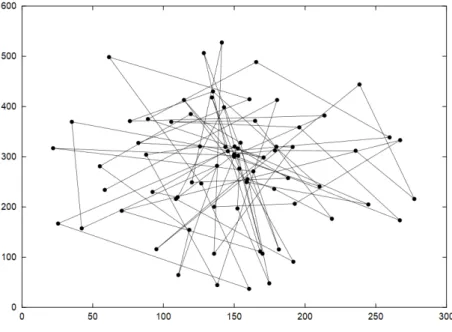
status of the simulation and the UABSs will adapt themselves according to the new conditions. An example of a snapshot with the different positions of the UABSs and ground users is illustrated in Figure 4.

Fig. 4. Example of a snapshot with 3 UABSs and 40 connected ground users.

The algorithm contains a total of eight different steps. As shown in Figure 5, the first four steps are executed once in the beginning and the four remaining steps are executed repeatedly during the simulation. Steps 1 to 4 are developed by [8] and steps 5 to 8 are created for this master’s dissertation. Important to note is that steps 5 to 8 will not be executed for scenario IV because nor the ground users, nor the UABSs will move. Moreover, because UABSs cannot be relocated in scenario I step 6 will only be executed in scenario II and III. Step 8 will only be carried out in scenario III since this is the only scenario in which extra UABSs can be activated or the redundant ones deactivated.

Fig. 5. General overview of the algorithm

Step 1 will generate random traffic. Users will be distributed randomly in the simulation area and assigned a certain bit rate as stated in section III-F.

In step 2, the algorithm generates the possible base station locations. The algorithm will try to place a drone above every user and mark that location as a possible position. If the location does not intersect with a building, it is marked as a potential coordinate.

In step 3, the network is generated based on the previous set of locations. This is an optimization phase in which users are connected to the best base station possible. In order to achieve this, the algorithm checks for each user to which active base station it can connect in the most efficient way in terms of path loss. If there are no active base stations present to which a user can connect to, a new base station will be activated if there are any left.

The fourth step will generate a facility, which will be located in the middle of the simulation area. In this manner, UABSs can save power because the UABSs have to cover the least distance on average. From this facility, the UABSs will depart to their assigned locations and return when the intervention has ended or when the battery of the drone carrier is empty.

Next, steps five to eight are executed every period of time. As mentioned before, these steps are considered in scenario IV. In step five, the algorithm moves all users depending on their behavior as discussed in section III-B. During this phase, each user’s location will be updated regarding their speed, direction and acceleration.

When scenario II and III are considered, the algorithm will assign new target locations for every drone and update their position accordingly considering their current speed, direction and location. These new target locations are based on the new positions of the users. In order to determine all possible locations, a modified global K-Means clustering algorithm is performed. The cost function (equation 1) consequently determines which cluster to visit by each UABS.

Next, the movement of all ground users and UABSs is processed. All the UABSs present in the simulation area try to connect as many ground users as possible.

Finally, the last step rearranges the network only when scenario III is employed. Here, extra UABSs left in the facility will be activated when required. The redundant UABSs will be deactivated and ordered to return to the facility.

When all steps are executed and the simulation is finished, the algorithm generates output files containing all the data of each snaptime. In addition to that, the mean value of every parameter generated during the whole simulation is also calculated. The different considered parameters are discussed in section III-G.

F. Scenario definitions

An existing area is used in order to simulate the different scenarios. The simulation area lies in the city center of Ghent as shown in Figure 6 and has a total area size of 4km2. The simulation area also includes the buildings present in the city in order to simulate the possibility of NLoS between UABSs

(15)

and ground users. Drones are assumed not to collide with each other nor with the existing buildings while moving.

Fig. 6. The city of Ghent as simulation area.

240 users are randomly distributed in the area and each re-quests a certain bit rate, either data (1 Mbps) or voice (64kbps) traffic. The amount of users together with a distribution of the data and voice traffic are based on realistic data from a Belgian mobile operator active in Belgium [8], [42]. Drones depart from a facility which is located in the center of the simulation area. In this manner, there is the highest probability that the drones have to cover the least distance on average.

The drone used for this analysis is the Microdrones’ md4-1000, based on the research performed by [8]. The speci-fications of this drone can be found in Table II and more information is given by [43]. The values in Table II consider a simple model. Moreover, weather conditions such as wind and rain which can affect the power consumption and speed are neglected.

TABLE II

PARAMETER VALUES OF THEmd4-1000DRONE CARRIER

Parameter Value Unit Average carrier speed 12 m/s Carrier power 13 Ampere Average carrier power usage 17.33 Ampere hour Carrier battery voltage 22.2 Volts

As for the base station, LTE femtocells are assumed to be employed and mounted on the drone carriers. Table III provides an overview of the assumed parameters of the LTE-Advanced link budget. It is also assumed that there is a constant interference margin between the different signals sent and received by the base stations and an omnidirectional antenna is used.

G. Evaluation parameters

To evaluate the proposed approach and algorithm, several evaluation parameters are considered for every simulation, which are listed in Table IV.

In this table the first parameter is the users coverage. This is the ratio of the amount of covered users to the total amount

TABLE III

LINK BUDGET TABLE FOR A FEMTOCELL BASE STATION. BASED ON[8], [42]

Parameter Value Unit

Frequency 2600 MHz

Maximum transmission power base station antenna 33 dBm Antenna gain base station 4 dBi

Soft handover gain 0 dB

Feeder loss base station 0 dB

Fade margin 10 dB

Interference margin 2 dB

Receiver Signal-to-Noise Ratio

1/3 QPSK -1.5 dB 1/2 QPSK 3 dB 2/3 QPSK 10.5 dB 1/2 16-QAM 14 dB 2/3 16-QAM 19 dB 1/2 64-QAM 23 dB 2/3 64-QAM 29.4 dB

Number of used subcarriers 301 -Number of total subcarriers 512

-Maximum bit rate 16.9 Mbps

Bandwidth 5 MHz

Noise figure mobile station 8 dB Implementation loss mobile station 0 dB

TABLE IV

OVERVIEW OF THE EVALUATION PARAMETERS FOR EACH SIMULATION

Parameter Short description

Users coverage The rate of connected users to the total amount of users in the area. Served capacity The amount of transferred data in

Mbps. Amount of disconnections per timestamp

The amount of users which lose their active communication link with a UABS.

Outage rate The rate of how many users were not served at all during the entire simulation to the total amount of users.

Mean service time The mean time of all users on how long they were served during the entire simulation.

Power usage The amount of power the network consumes.

Amount of active UABSs Amount of drones active in the area.

Facility size Amount of UABSs stored in the facility and able to be activated

of users in the area. The second parameter is related to the users coverage, which is the capacity of the network. This is the amount of transferred data for a certain timestamp and is calculated for the total network as well as for the average capacity of each UABS. The users coverage and the capacity of the network will indicate how well the network performs and is very important since the overall goal of this research is maximizing the amount of covered users.

The third parameter is the amount of disconnections per timestamp. This value expresses how many ground nodes lose their communication link per timestamp. The users which were handed over are not taken into account by this parameter. This parameter will be influenced by the amount of active UABSs and amount of ground nodes in the area among others. Other important parameters are the outage rate and the mean service time. The outage rate is a value that indicates how many users

(16)

were not served at all during the whole intervention compared to the total amount of users. This value is particularly inter-esting to evaluate the difference between a static deployment (scenario I and IV) and a dynamic deployment (scenario II and III). The mean service time on the other hand is a parameter that defines how long users were served during the entire simulation. This is an average value of all the users present in the area and should also be influenced by the type of scenario. The sixth output parameter considered is the power usage. This parameter is calculated for both the mean power usage for each UABS as for the sum of the total power usage of each UABS combined. The power usage considers both the energy for the drone carrier to remain in the air and the energy for the base station to provide a communication link to the ground nodes. The amount of active UABSs is also considered for evaluation. This parameter is a value that denotes how many UABSs are active in the air for a certain timestamp and how many UABSs are actually being used. The last parameter is the facility size and defines how many UABSs are stored in the facility and are able to be deployed.

IV. RESULTS&DISCUSSION

An analysis on the performance of the network is performed to evaluate the behavior of combining a static and dynamic deployment. In doing so, the proposed scenarios were com-pared among each other. In each scenario, a standardized experiment was carried out in which all input parameters were kept constant except for the investigated parameter. An overview of the default input parameters can be found in Table V. Unless mentioned otherwise, the users’ walking behavior for the analyses is walking type D, in which users have a variable speed and variable direction.

TABLE V

OVERVIEW STANDARD INPUT PARAMETERS FOR EACH SIMULATION

Input parameter Value Unit Number of users 240 -Facility size 40 -Fly height 90 m Maximum fly height 90 m Height above building 4 m Simulation time 1800 s

Snaptime 30 s

Shifttime 45 s

Walking behavior D

-A. Dynamic ground users

There is a big difference in how the network behaves when ground users stand still or move continuously in the simulation area. A comparison is made between the four scenarios. The difference between the scenarios of the users coverage in time is visualized in Figure 7. First of all, it can be seen that when the ground users are fixed (scenario IV), the UABSs will also hover on the same location during the entire simulation. The users coverage is 57% for scenario IV during the whole simulation time. Secondly, it can be concluded that a more realistic scenario (scenario I, II and III) where

40 50 60 70 0 180 360 540 720 900 1080 1260 1440 1620 1800 Time (s) Co v er age (%)

Scenario I Scenario II Scenario III Scenario IV

Users coverage

Fig. 7. Comparison of users coverage in a network with moving (scenario I, II and III) and fixed users (scenario IV) in function of the time.

ground users move around have an apparent influence on the network behavior. Users moving around the simulation area lead to a negative impact on the overall network performance when UABSs hover at fixed locations (scenario I). After 1000 seconds the users coverage drops from 57% down to 44% for scenario I. This means that a difference of around 13% is noticed between scenario I and IV at 1000 seconds. To overcome this problem, UABSs can be relocated as performed in scenario II and III. For scenario II, the users coverage decreases from 57% to 55% in 1000 seconds, resulting in a difference of only 2% between scenario II and IV. The difference between scenario I and II indicates that is not desirable to keep UABSs static in a more realistic network where ground users move around. In scenario II, the UABSs are able to relocate themselves to better locations according to the current needs of the network. Because users can get more spread out, extra UABSs are being deployed in scenario III when there are still any left in the facility. This results in a users coverage of around 64%, which is even better compared to scenario IV.

The improvement in users coverage of scenario III in com-parison to scenario II is due to the fact that extra UABSs can be activated up until the maximum amount of UABSs stored in te facility are deployed, which is in this case 40. In scenario II, the amount of UABSs to be activated is determined in the very beginning of the simulation and remains fixed throughout the entire simulation as shown in Figure 8a. Scenario I, II and IV use nearly the same amount of active UABSs (34 UABSs) while scenario III uses the maximum amount of deployable UABSs (40 UABSs). This means that despite the better performance of scenario III in terms of users coverage, a difference in power usage of around 2.7kW is observed with scenario II in Figure 8b. Additionally, in Figure 8b it can be seen that a small increase in power usage (0.11kW for scenario I and 0.04kW for scenario II) was also observed between scenario IV and and both scenarios I and II. This difference is a result of the fact that the ground users have other positions and thus may be located further away. Therefore the UABSs adapt their transmitted power resulting in a higher energy consumption.

So, it is shown that a remarkable impact on the behavior of the network follows from the fact that ground users are able to move, especially when the UABSs remain static. Scenario

(17)

IV, in which the users remain at a fixed location, is considered not to be realistic, so this scenario will not be examined in the remaining sections of the analysis.

Fig. 8. Comparison of a network with moving (scenario I, II and III) and fixed users (scenario IV): (a) the amount of active UABSs in the network in function of the time and (b) the total power usage of the network in function of the time

B. Walking behavior

As described in section III-B, the ground users can have four different walking behaviors. All four types of walking behavior are considered to analyze their impact on the network. The influence on the users coverage is visualized in Figure 9. One important outcome is that the mean users coverage performed worse for scenario I when walking type A and B is considered. The users coverage rate is around 6% worse when comparing walking type A and B to walking type C and D. An explanation for this is that users have less chance to get a new connection since their direction remains fixed and are therefore limited to obtain a connection via the UABSs they come across. When a variable direction is configured (walking type C), a higher probability exists for the users to come and stay in range of a UABS which can result in a higher mean users coverage.

In contrast to scenario I, the mean users coverage is better for scenario II and III in case of a fixed direction (walking type A and B) compared to a variable direction (walking type C and D). A difference of nearly 20% is observed since a less chaotic walking pattern of all users was present. As a result, it is easier for the UABSs to follow the ground users. The impact of a variable speed (walking type B and D) on the mean users coverage can also be seen in Figure 9. It is found that a variable speed has almost no effect on the mean users coverage for all scenarios (< 1%).

39.36 75.65 81.11 45.61 55.71 63.06 38.84 75.55 81.96 45.85 56.28 63.24

Walking type C Walking type D

Walking type A Walking type B

Scenario I Scenario II Scenario III Scenario I Scenario II Scenario III 0 25 50 75 100 0 25 50 75 100 Mean co v er age (%)

Fig. 9. Influence of the four different walking behaviors on the mean users coverage.

Fig. 10. Influence of the facility size on the users users coverage (a) and the amount of active UABSs per timestamp (b).

C. Influence of the UABSs

Increasing the facility size will result in a better performance of the network as more UABSs can be deployed and thus more users can be served. In Figure 10a, the influence on the mean users coverage of the entire duration of the simulation versus the facility size is depicted. Scenario I performed worse compared to the other two scenarios, since UABSs cannot relocate themselves. As can be expected, the mean users coverage increases when the facility size increases and eventually the curve flattens out. The mean users coverage for this scenario will eventually reach a value of 86.2% in case 240 UABSs are able to be deployed. For scenario II, the mean users coverage when the facility size is equal to 20 UABSs is very similar to mean users coverage of scenario III (± 35%). This is due to the fact that almost the same amount of active UABSs are deployed in the very beginning of the scenario as can be seen in Figure 10b. When only 20 UABSs and 240 users are present, a situation occurs where more UABSs are

(18)

requested which causes a higher amount of UABSs in the very beginning of the scenario. As the facility size increases, less UABSs will be deployed from the very beginning, resulting in a worse performance compared to scenario III.

When more UABSs can be deployed, more UABSs are being activated in scenario II. This curve will flatten out and scenario II will reach eventually a mean users coverage of 96% when a facility size of 220 or more is present. Scenario III on the other hand will reach the same mean users coverage of almost 96% for 88 active UABSs are present (for a facility size equal to 100 UABSs). The users coverage remains the same when more UABSs are available to deploy. This indicates that no more than around 88 UABSs are required to be stored in the facility to obtain such a high mean users coverage as depicted in Figure 10b. Important to note is that a small portion, namely 4% of the users, will always remain uncovered due to their unfavorable locations at which it is impossible to reach these users.

D. Fly height

This section researches the effect of the fly height on the users coverage rate. The height margin between the surface and the drone is hereby considered. It is important to note that a location is set unfeasible if the required fly height is smaller than the height of a building plus the height above the roof of the building, which is in this case 4 meters as described in table V. 0 20 40 60 80 20 40 60 80 100 120 140 160 180 Height (m) Mean co v er age (%)

Scenario I Scenario II Scenario III

Mean users coverage

Fig. 11. Influence of the fly height of the UABSs on the mean users coverage.

The influence of the fly height on the mean users coverage rate is shown in Figure 11. As the altitude increases, the probability of connections between the users and the base stations in LoS increases as well. This means that there is a lower chance that the signal travels trough a building with a lower path loss as result. On the other hand, there is a limitation on the fly height since the distance between base station and ground user will increment, leading to a higher path loss. These two effects are contradictory. At first, the positive impact of more connections in the LoS predominates. This results in a decrease of path loss, with an increasing fly height causing a higher mean coverage rate, as illustrated in Figure 11. However, the gain in mean coverage rate will become less and less as the height increases from a certain

point. This is due to the fact that the higher distance starts outweighing the positive effect of a higher amount of LoS links between the ground users and the base stations [16]. It is derived from Figure 11 that scenario I will reach a maximum coverage rate of 50.4% at an altitude of 120m. In addition, the mean coverage rate for both scenario II and III will reach a maximum of respectively 64.6% and 74.3% at an altitude of 140m.

E. General comparison of the three proposed scenarios Finally, an overview of the most important parameters is shown in Table VI which compares all three scenarios (scenario I, II and III). The results from this table are obtained with the optimal altitudes of the UABSs as discussed in section IV-D.

From this table it can be derived that scenario I generally performs worse compared to scenario II and III in the context of technical performance parameters. Scenario II obtained a mean users coverage of 64.6% which is around 14% better compared to the mean users coverage of 50.4% for scenario I. As a result, the mean served capacity per UABS (3.35 Mbps versus 4.35 Mbps for scenario I and II) and the total served capacity (111.1 Mbps versus 142.2 Mbps for scenario I and II) is also considerably higher. This difference is accompanied with a lower power usage for scenario II (13.1 kW) compared to scenario I (13.3 kW). On top of that, the outage rate and the mean service time per user is better for scenario II (1.3% and 1162s respectively) compared to scenario I (10.1% and 903s respectively). Scenario I performs only better on the mean amount of disconnections per timestamp as 9.0 users are disconnected in scenario I compared to 13.5 in scenario II. The better performance is achieved because less users are connected. However, research demonstrates that when more the facility size increases, scenario I performs worse on this aspect parameter as well. Yet, this is not shown in this article. Because of all this, a major conclusion is that it is undesirable in terms of efficiency to keep the UABSs fixed when moving ground users are present in the network.

Scenario III scores even better compared to scenario I. The users coverage of scenario III is 74.3 %, which is an improvement of 24% to scenario I. This results in a higher total served capacity of 163.78 Mpbs, better outage rate of 0.5% and mean service time of 1340s for scenario III. In addition, the mean power usage is lower for scenario II and III compared to scenario I as a difference of 2 Watts is noted. This small difference results in an overall lower total consumption of energy and the difference will further increase as more UABSs are deployed. The lower mean power usage per UABS is due to the fact that ground users are less far away and thus less transmission power is required. The better performance of scenario III comes at a cost, since a power usage of 16 kW is present, resulting in a difference of almost 2.7 kW compared to scenario I.

Comparing scenario II and III, scenario III performs better in terms of mean users coverage, total served capacity and outage rate. Furthermore, a lower facility size is required for

(19)

TABLE VI

COMPARISON OF SCENARIOI, IIANDIIIWITH THE MOST IMPORTANT PARAMETERS WITH AN ALTITUDE OF120M FOR SCENARIOIAND140M FOR SCENARIOIIANDIII.

Scenario II (120m) Scenario II (140m) Scenario III (140m) Overall network performance

Mean users coverage (%) 50.40 64.57 74.32 Mean served capacity per UABS (Mbps) 3.35 4.35 4.11

total served capacity (Mbps) 111.10 142.23 163.78 UABSs

Amount of active UABSs (-) 33.15 32.70 39.87 Total power usage (kW) 13,3 13.1 16.0 Mean power usage per UABS (W) 402 400 400 Mean transmitpower (dBm) 31.37 30.69 30.22

Users

Mean amount of disconnections per timestamp (-) 9.00 13.50 13.31

Outage rate (%) 10.06 1.31 0.46

Mean service time (s) 903.39 1161.60 1340.33

scenario III, as discussed in section IV-C. This demonstrates that an approach at which UABSs are able to be deployed dynamically according to the current requirements of the network of each snapshot is more efficient. However, the cost of the better performance is a higher power consumption (2.9 kW).

V. CONCLUSION

In this master’s dissertation a new approach for UAV-aided network applications in which ground users are moving is presented. More specifically, a combination of a static and dynamic deployment is introduced for this manner. UABSs have the ability to hover on a certain location and move to other interesting locations as well. To simulate the movement of the ground users, the smooth random mobility model is used. A modified version of the global K-means clustering algorithm is used to group the moving ground users and a cost-function evaluated each cluster.

It can be concluded that moving ground users have a clear negative impact on the network when UABSs remain fixed. To encounter this, UABSs will be relocated by utilizing a modified global K-means clustering algorithm in combination with a cost-function. The cost-function takes the user density, amount of users and location of the cluster into account. This results in an improvement of 14% in users coverage when optimal heights were configured for both approaches (120 meters for fixed UABSs (scenario I) and 140 meters for dynamic UABSs (scenario II)). The better performance for scenario II compared to scenario I was performed while the same amount of UABSs were activated. Furthermore, it was shown that by having the ability to deploy extra UABSs if required and deactivating the redundant ones (scenario III), the network performances were improved even more as an increase of 24% in mean users coverage is noted compared to scenario I (with an optimal flying altitude of 140 meters for scenario III). This however comes with a higher power consumption of 2.7 kW. The way on how the users move have also an apparent effect. To investigate such a case, four types of walking behavior were researched, each to represent another situation. Based on the results, it is clear that a situation where

the speed is variable has a rather small impact on the users coverage (< 1%). On the other hand, a variable direction has a considerable influence on the users coverage (± 6%).

Results show there is a huge potential in moving and de-ploying UABSs in wireless network communication systems. However further research is still required. A simple model for the drone carrier was utilized. In order to obtain more specific results, it is suggested to develop a more sophisticated model. This model may also include influences of the weather as up until now, this aspect is neglected. In addition, one of the main drawbacks is the fact that the UABSs are always positioned behind their assigned users due to the time intervals between the different snapshots. Investigating how to predict the user’s positions by employing machine learning could be one possible solution for this particular problem. Machine learning requires also a lower computational time [29], [30], which can lead to a higher updating frequency of the UABSs’ locations. Finally, a more advanced mobility model including other situations and faster moving users (e.g. cars and trains) could be another interesting feature to investigate.

REFERENCES

[1] Silvia Mignardi and Roberto Verdone. UAV - Aided B5G Networks. European Cooperation in Science and Technology, 2017.

[2] Bin Li, Zesong Fei, and Yan Zhang. UAV communications for 5G and beyond: Recent advances and future trends. IEEE Internet of Things Journal, 6(2):2241–2263, apr 2019.

[3] Long Zhang, Hui Zhao, Shuai Hou, Zhen Zhao, Haitao Xu, Xiaobo Wu, Qiwu Wu, and Ronghui Zhang. A survey on 5g millimeter wave communications for uav-assisted wireless networks. IEEE Access, 7:117460–117504, 2019.

[4] Milan Erdelj, Enrico Natalizio, Kaushik R. Chowdhury, and Ian F. Aky-ildiz. Help from the Sky: Leveraging UAVs for Disaster Management, jan 2017.

[5] Paulo V. Klaine, Jo˜ao P. B. Nadas, Richard D. Souza, and Muhammad A. Imran. Distributed Drone Base Station Positioning for Emergency Cel-lular Networks Using Reinforcement Learning. Cognitive Computation, 10(5):790–804, oct 2018.

[6] Mohammad Mozaffari, Walid Saad, Mehdi Bennis, and Merouane Debbah. Drone Small Cells in the Clouds: Design, Deployment and Performance Analysis. pages 1–6. Institute of Electrical and Electronics Engineers (IEEE), mar 2016.

[7] Ahmad Sawalmeh, Noor Othman, and Hazim Shakhatreh. Efficient Deployment of Multi-UAVs in Massively Crowded Events. Sensors, 18(11):3640, oct 2018.

(20)

[8] Margot Deruyck, Jorg Wyckmans, Wout Joseph, and Luc Martens. Designing UAV-aided emergency networks for large-scale disaster sce-narios. Eurasip Journal on Wireless Communications and Networking, 2018(1), dec 2018.

[9] Qingqing Wu, Yong Zeng, and Rui Zhang. Joint trajectory and communication design for multi-UAV enabled wireless networks. IEEE Transactions on Wireless Communications, 17(3):2109–2121, mar 2018. [10] Margot Deruyck, Alberto Marri, Silvia Mignardi, Luc Martens, Wout Joseph, and Roberto Verdone. Performance evaluation of the dynamic trajectory design for an unmanned aerial base station in a single fre-quency network. In IEEE International Symposium on Personal, Indoor and Mobile Radio Communications, PIMRC, volume 2017-Octob, pages 1–7. Institute of Electrical and Electronics Engineers Inc., feb 2017. [11] Ahmad H. Sawalmeh, Noor Shamsiah Othman, Hazim Shakhatreh, and

Abdallah Khreishah. Wireless Coverage for Mobile Users in Dynamic Environments Using UAV. IEEE Access, 7:126376–126390, 2019. [12] Hazim Shakhatreh, Ahmad H. Sawalmeh, Ala Al-Fuqaha, Zuochao Dou,

Eyad Almaita, Issa Khalil, Noor Shamsiah Othman, Abdallah Khreishah, and Mohsen Guizani. Unmanned Aerial Vehicles (UAVs): A Survey on Civil Applications and Key Research Challenges, 2019.

[13] Shuhang Zhang, Hongliang Zhang, Qichen He, Kaigui Bian, and Lingyang Song. Joint Trajectory and Power Optimization for UAV Relay Networks. IEEE Communications Letters, 22(1):161–164, jan 2018. [14] Ilker Bekmezci, Ozgur Koray Sahingoz, and S¸amil Temel. Flying

Ad-Hoc Networks (FANETs): A survey, may 2013.

[15] Long D. Nguyen, Khoi K. Nguyen, Ayse Kortun, and Trung Q. Duong. Real-Time Deployment and Resource Allocation for Distributed UAV Systems in Disaster Relief. In IEEE Workshop on Signal Processing Advances in Wireless Communications, SPAWC, volume 2019-July. Institute of Electrical and Electronics Engineers Inc., jul 2019. [16] German Castellanos, Margot Deruyck, Luc Martens, and Wout Joseph.

Performance evaluation of direct-link backhaul for UAV-aided emer-gency networks. Sensors (Switzerland), 19(15), aug 2019.

[17] Kenichi Mase and Hiraku Okada. Message communication system using unmanned aerial vehicles under large-scale disaster environments. In IEEE International Symposium on Personal, Indoor and Mobile Radio Communications, PIMRC, volume 2015-Decem, pages 2171– 2176. Institute of Electrical and Electronics Engineers Inc., dec 2015. [18] Lien Shao-Yu and Chen Kwang-Cheng. Toward Ubiquitous Massive

Accesses in 3GPP Machine-to-Machine Communications. IEEE Com-munications Magazine, 2011.

[19] Mohammad Mozaffari, Walid Saad, Mehdi Bennis, and Merouane Debbah. Mobile Internet of Things: Can UAVs Provide an Energy-Efficient Mobile Architecture? jul 2016.

[20] Jun Xu, Gurkan Solmaz, Rouhollah Rahmatizadeh, Damla Turgut, and Ladislau Boloni. Internet of Things Applications: Animal Monitoring with Unmanned Aerial Vehicle. oct 2016.

[21] Jiangbin Lyu, Yong Zeng, Rui Zhang, and Teng Joon Lim. Placement Optimization of UAV-Mounted Mobile Base Stations. IEEE Communi-cations Letters, 21(3):604–607, mar 2017.

[22] R. Irem Bor-Yaliniz, Amr El-Keyi, and Halim Yanikomeroglu. Efficient 3-D placement of an aerial base station in next generation cellular networks. In 2016 IEEE International Conference on Communications, ICC 2016. Institute of Electrical and Electronics Engineers Inc., jul 2016. [23] Elham Kalantari, Halim Yanikomeroglu, and Abbas Yongacoglu. On the number and 3D placement of drone base stations in wireless cellular networks. In IEEE Vehicular Technology Conference, volume 0. Institute of Electrical and Electronics Engineers Inc., jul 2016.

[24] Elham Kalantari, Muhammad Zeeshan Shakir, Halim Yanikomeroglu, and Abbas Yongacoglu. Backhaul-aware robust 3D drone placement in 5G+ wireless networks. In 2017 IEEE International Conference on Communications Workshops, ICC Workshops 2017, pages 109–114. Institute of Electrical and Electronics Engineers Inc., jun 2017. [25] D. Alejo, J. A. Cobano, G. Heredia, and A. Ollero. Collision-free

4D trajectory planning in Unmanned Aerial Vehicles for assembly and structure construction. Journal of Intelligent and Robotic Systems: Theory and Applications, 73(1-4):783–795, oct 2014.

[26] Silvia Mignardi and Roberto Verdone. On the Performance Improvement of a Cellular Network Supported by an Unmanned Aerial Base Station. In Proceedings of the 29th International Teletraffic Congress, ITC 2017, volume 2, pages 7–12. Institute of Electrical and Electronics Engineers Inc., oct 2017.

[27] Hassan Daryanavard and Abbas Harifi. UAV Path Planning for Data Gathering of IoT Nodes: Ant Colony or Simulated Annealing

Opti-mization. In Proceedings of 3rd International Conference on Internet of Things and Applications, IoT 2019. Institute of Electrical and Electronics Engineers Inc., apr 2019.

[28] Qingqing Wu, Liang Liu, and Rui Zhang. Fundamental trade-offs in communication and trajectory design for UAV-enabled wireless network. IEEE Wireless Communications, 26(1):36–44, feb 2019.

[29] Rozhina Ghanavi, Elham Kalantari, Maryam Sabbaghian, Halim Yanikomeroglu, and Abbas Yongacoglu. Efficient 3D Aerial Base Sta-tion Placement Considering Users Mobility by Reinforcement Learning. jan 2018.

[30] Liang Liu, Shuowen Zhang, and Rui Zhang. CoMP in the Sky: UAV Placement and Movement Optimization for Multi-User Communica-tions. IEEE Transactions on Communications, 67(8):5645–5658, aug 2019.

[31] Kuldeep Singh and Anil Kumar Verma. Adaptability of Various Mobility Models for Flying AdHoc Networks—A Review. pages 51–63. Springer, Singapore, 2018.

[32] G. Andr´ea Ribeiro and C. Sofia Rute. A survey on mobility models for wireless networks. 2011.

[33] Radhika Ranjan Roy. Handbook of Mobile Ad Hoc Networks for Mobility Models. Springer US, Boston, MA, 2011.

[34] Kardi Teknomo. Microscopic Pedestrian Flow Characteristics: Devel-opment of an Image Processing Data Collection and Simulation Model. PhD thesis, Tohoku University, 2002.

[35] Stefan Buchm¨uller and Ulrich Weidmann. Parameters of pedestrians, pedestrian traffic and walking facilities. IVT Schriftenreihe, 132, 2006. [36] Satish Chandra and Anish Kumar Bharti. Speed Distribution Curves for Pedestrians During Walking and Crossing. Procedia - Social and Behavioral Sciences, 104:660–667, dec 2013.

[37] Ngoc-Huynh Ho, Phuc Truong, and Gu-Min Jeong. Step-Detection and Adaptive Step-Length Estimation for Pedestrian Dead-Reckoning at Various Walking Speeds Using a Smartphone. Sensors, 16(9):1423, sep 2016.

[38] Aristidis Likas, Nikos Vlassis, and Jakob J. Verbeek. The global k-means clustering algorithm. Pattern Recognition, 36(2):451–461, feb 2003.

[39] Mung Chiang, Prashanth Hande, Tian Lan, and Chee Wei Tan. Power Control in Wireless Cellular Networks. now Publishers Inc., Hanover, 2008.

[40] Karl L¨ow. Comparison of urban propagation models with CW-measurements. In IEEE Vehicular Technology Conference, volume 1992-May, pages 936–942. Institute of Electrical and Electronics Engineers Inc., 1992.

[41] Emmeric Tanghe, Wout Joseph, Leen Verloock, Luc Martens, Henk Capoen, Kobe Van Herwegen, and Wim Vantomme. The industrial indoor channel: Large-scale and temporal fading at 900, 2400, and 5200 MHz. IEEE Transactions on Wireless Communications, 7(7):2740–2751, jul 2008.

[42] Margot Deruyck, Wout Joseph, Emmeric Tanghe, and Luc Martens. Reducing the power consumption in LTE-Advanced wireless access net-works by a capacity based deployment tool. Radio Science, 49(9):777– 787, sep 2014.

[43] Microdrones. Fully integrated systems for professionals, 2020. Retrieved from https://www.microdrones.com/en/integrated-systems/.

(21)

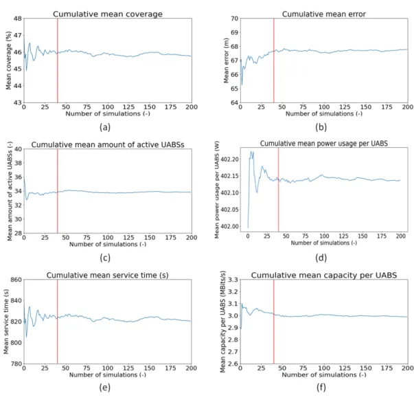
3.1 General concept . . . 25 3.2 Dynamic behavior of ground nodes . . . 26 3.3 Behavior of UABSs . . . 28 3.4 Scenario definitions . . . 32 3.5 Scenario types . . . 33 3.5.1 Scenario I . . . 33 3.5.2 Scenario II . . . 34 3.5.3 Scenario III . . . 35 3.5.4 Scenario IV . . . 35 3.6 Evaluation parameters . . . 36 3.6.1 Input parameters . . . 36 3.6.2 Output parameters . . . 37 4 Deployment tool 39 4.1 Algorithm . . . 39 4.1.1 Steps 1 - 4: Initialization . . . 40 4.1.2 Step 5: Move users . . . 41 4.1.3 Step 6: Move drones . . . 41 4.1.3.1 Clustering algorithm . . . 42 4.1.3.2 Move drones algorithm . . . 43 4.1.4 Step 7: Process movement . . . 45 4.1.4.1 Step 7.3: Covered users . . . 46 4.1.4.2 Step 7.4: Uncovered users . . . 47 4.1.4.3 Step 7.6: Outliers . . . 47 4.1.5 Step 8: Rearrange the network . . . 52 4.1.5.1 Step 8.1: Deactivate UABSs . . . 52 4.1.5.2 Step 8.2: Deploy extra UABSs . . . 53 4.1.6 Output generation . . . 54 4.2 Convergence . . . 54 4.2.1 Scenario I . . . 55 4.2.2 Scenario II . . . 57 4.2.3 Scenario III . . . 58 4.2.4 Scenario IV . . . 59

(23)

CONTENTS xxv

5 Results & discussion 61

5.1 General setup . . . 61 5.2 Ground users . . . 62 5.2.1 Dynamic ground users . . . 63 5.2.2 Walking speed . . . 65 5.2.3 Walking behavior . . . 67 5.2.4 Amount of ground users . . . 70 5.3 Fly height . . . 73 5.4 Influence of the UABSs . . . 75 5.4.1 Facility size . . . 75 5.4.2 Speed drone carrier . . . 79 5.5 Snaptime . . . 81 5.6 General comparison of the three employed scenarios . . . 84 5.7 Final results remark . . . 86

6 Conclusion 90

(24)

List of Figures

2.1 Simple Mobile Ad Hoc Network . . . 4 2.2 Network architecture of an integrated airborne communication network . . . 6 2.3 A UAV in a public safety scenario . . . 7 2.4 Example of a travelling pattern using the Random Walk Mobility Model . . . 9 2.5 Example of a travelling pattern using the Random Direction Model . . . 10 2.6 Change of mean angle near the edges (in degrees) in the Gauss-Markov mobility mode . . . 11 2.7 City section mobility model example . . . 12 2.8 Example of user movement in Reference Point Group Mobility Model . . . 12 2.9 Illustration of the spiral algorithm . . . 18 2.10 Example of a dendrogram . . . 21 2.11 Example of the K-means clustering algorithm . . . 23 3.1 Schematic overview of the static scenario developed in the WAVES research group . . . 26 3.2 Adapted schematic overview of a static and a dynamic scenario combined . . . 26 3.3 Travel path of a single ground node in the simulation area . . . 27 3.4 Power control principle applied . . . 28 3.5 Determination of the coverage range . . . 29 3.6 Example of the global K-Means clustering algorithm . . . 30 3.7 The different parameters for the cost-function to determine which cluster to visit . . . 32 3.8 The city of Ghent as simulation area. . . 32 3.9 Principle of scenario II . . . 35 4.1 Example of a snapshot . . . 39 4.2 General overview of the algorithm . . . 40 4.3 Algorithm to move users in the simulation area . . . 42 4.4 Algorithm to move the drones in the simulation area . . . 44 4.5 General overview algorithm to process the movement of the users and UABSs in the

simu-lation area . . . 45 4.6 Algorithm to process the covered users . . . 46

(25)

LIST OF FIGURES xxvii

4.7 Algorithm to process uncovered users . . . 48 4.8 Algorithm to process outliers . . . 49 4.9 Principle of Situation A . . . 49 4.10 Algorithm to process outliers in Situation A . . . 50 4.11 Principle of Situation B . . . 51 4.12 Algorithm to process outliers in Situation B . . . 51 4.13 Algorithm to deactivate UABSs . . . 52 4.14 Algorithm to deploy extra UABSs . . . 53 4.15 Cumulative means in function of the number of simulations for scenario I . . . 56 4.16 Cumulative means in function of the number of simulations for scenario II . . . 57 4.17 Cumulative means in function of the number of simulations for scenario III . . . 59 4.18 Cumulative means in function of the number of simulations for scenario IV . . . 60 5.1 Comparison of the users coverage and the total served capacity of the network with fixed

and moving ground users . . . 63 5.2 Comparison of a network with moving (scenario I, II and III) and fixed users (scenario IV):

(a) the amount of active UABSs in the network in function of the time and (b) the total power usage of the network in function of the time . . . 65 5.3 Influence of the walking speed of the users on the mean users coverage and the mean capacity

of each UABS. . . 66 5.4 Impact of the walking speed of the users on the mean amount of disconnections per timestamp. 67 5.5 Influence of the walking speed of the users on the outage rate. . . 68 5.6 Influence of the four different walking behaviors on the mean users coverage. . . 68 5.7 Influence of the four different walking behaviors on the outage rate. . . 69 5.8 Influence of the amount of users on the mean users coverage. . . 70 5.9 Influence of the amount of users on the mean amount of active UABSs per timestamp . . . . 71 5.10 Influence of the amount of users on the total served capacity of the network. . . 72 5.11 Influence of the amount of users on the average service time and on the outage rate . . . 73 5.12 Influence of the fly height of the UABSs on the average users coverage. . . 74 5.13 Influence of the fly height of the UABSs on the outage rate. . . 74 5.14 Influence of the facility size on the users coverage and the amount of active UABSs per

timestamp . . . 76 5.15 Influence of the facility size on the total power usage of the network. . . 77 5.16 Influence of the facility size on the mean amount of disconnections per timestamp . . . 78 5.17 Influence of the facility size on the mean service time per user. . . 78 5.18 Influence of the facility size on the outage rate of the network . . . 79