PM10: Equivalence study 2006 : Demonstration of equivalence for the automatic PM10 measurements in the Dutch National Air Quality Monitoring Network : A technical background report | RIVM

PM10: Equivalence study 2006

RIVM Report 680708002/2008

PM

10

: Equivalence study 2006

Demonstration of equivalence for the automatic PM

measurements in the Dutch

National Air Quality Monitoring Network

A technical background report

R. Beijk D. Mooibroek J. van de Kassteele R. Hoogerbrugge Contact: Ruben Beijk

Laboratory for Environmental Monitoring Ruben.Beijk@rivm.nl

This investigation has been performed by order and for the account of the Directorate-General for the Environment, within the framework of the Dutch National Air Quality Monitoring Network

© RIVM 2008

Parts of this publication may be reproduced, provided acknowledgement is given to the 'National Institute for Public Health and the Environment', along with the title and year of publication.

Abstract

PM10: Equivalence study 2006

An equivalence study is carried out with the aim of ensuring the quality of PM10 measurements in the

Dutch National Air Quality Monitoring Network (NAQMN). The results have led to an improvement in the quality of the measurements and introduce an appropriate calibration for the PM10 measurements

in the NAQMN. The resulting relative measurement uncertainty for particulate matter (PM10)

measurements – performed by configurations currently in use in the NAQMN – is approximately 17%. In the NAQMN, PM10 is measured at various locations across the Netherlands using automatic

beta-adsorption monitors. European (EU) legislation allows this measurement method if equivalence with the official reference method (gravimetric measurements) is demonstrated. The NAQMN comprises various measurement configurations, and equivalence has been determined for each configuration. A distinction is made between three different devices and between urban and rural sites.

This study is primarily based on the equivalence guideline as recommended by the Clean Air For Europe (CAFE) steering group. Orthogonal regression is used in all cases to determine equivalency, and in situations with an insignificant intercept, orthogonal regression without intercept is applied. The equations for orthogonal regression without intercept and the corresponding uncertainty are presented. The technical background information of the steps taken to demonstrate equivalence is elaborated on in more detail in this report.

Key words:

Rapport in het kort

PM10: Equivalentie studie 2006

In een zogeheten equivalentiestudie door het RIVM is de onzekerheidsfactor bepaald tussen de fijnstofmetingen (PM10) in het Landelijk Meetnet Luchtkwaliteit (LML) en de Europese

referentiemethode. De in de equivalentiestudie bepaalde meetonzekerheid van de huidige PM10

-meetinstrumenten in het meetnet bedraagt circa 17 procent. De in de Europese richtlijn vermelde maximaal toegestane onzekerheid is 25 procent. De equivalentiestudie is uitgevoerd om de kwaliteit van deze fijnstofmetingen in Nederland te waarborgen. Tevens heeft de studie geleid tot verbeteringen in de kwaliteit van de PM10-metingen in het LML.

In dit rapport wordt de technische achtergrond van de gevolgde stappen en de bijbehorende resultaten nader beschreven. Het LML meet PM10 op circa veertig locaties met behulp van automatische

bèta-adsorptiemonitoren. Hoewel deze methode afwijkt van de voorgeschreven referentiemethode, staat de Europese regelgeving deze toe mits gelijkwaardigheid met de referentiemethode wordt aangetoond. Dat is voor de verschillende PM10-meetopstellingen in het meetnet onderzocht en aangetoond. Hierbij is

onderscheid gemaakt tussen drie apparaattypen en tussen meetlocaties binnen en buiten het stedelijk gebied.

Het equivalentieonderzoek is grotendeels gebaseerd op de guideline die de Europese werkgroep Clean Air For Europe (CAFE) aanbeveelt. Op één onderdeel is daarvan afgeweken. Voor dat onderdeel is een alternatieve wiskundige methode ontwikkeld, die ook in deze studie wordt gepresenteerd.

Trefwoorden:

Contents

2.3 Determination of relative measurement uncertainty 15

2.4 Testing equivalence 16

3 Reference method 17

3.1 Characteristics 17

3.2 Validation 17

3.3 Comparability 18

3.4 Correction of samples weighed at 43% relative humidity 19

4 Candidate method 21 4.1 Characteristics 21 4.2 Validation 22 4.3 Comparability 22 4.4 Recalculation 22 5 Equivalence results 25 5.1 Data characteristics 25

5.2 Calibration and equivalence of the four candidate methods 25

5.3 Level of representativeness 29

5.4 Aerosols (ammonium nitrate) 33

6 Conclusion 35

References 37

Appendix A: Orthogonal regression 39

Appendix B: LVS Filter comparability 43

Appendix C: LVS inside or outside an outdoor housing 47

Summary

Monitoring of the national air quality in the Netherlands is carried out within the framework of the National Air Quality Monitoring Network (LML). This monitoring network is operated by the Dutch National Institute for Public Health and the Environment (RIVM) and comprises approximately 49 monitoring stations distributed throughout the Netherlands. Particulate matter (PM10) at 40 of these

stations is measured using automated beta-gauge monitors. European (EU) legislation, however, prescribes the gravimetric method as the reference method (RM), although methods other than the RM are allowed when equivalence with the RM is demonstrated. The RIVM therefore performed an equivalence study, expanded with additional experiments, to improve the quality of the PM10

measurements.

The equivalence study is carried out following the guideline of the European Commission (EC) Working Group on Guidance for the Demonstration of Equivalence (2005). This report elaborates on the steps that are taken to demonstrate equivalence. Results of these steps are presented and discussed.. Both the final calibration factors and resulting measurement uncertainty are presented. Equivalence is demonstrated on the basis of these results.

Calibration factors for beta-gauge devices are determined for various configurations. Four candidate methods are defined – the new FH62 I-R monitor at rural sites, the same monitor at urban sites, the old FH62 I-N monitor with an optimized heating system at urban sites and the old FH62 I-N model with the original heating system at urban sites. Each configuration is characterized by a distinct calibration function, which varies between 1.17x (FH62 I-N old heating system) and 1.30x (FH62 I-N optimized heating system). Only the new FH62 I-R at rural sites shows a calibration with an intercept

(1.17x + 2.7 μg/m3). For the FH62 I-R at urban sites a calibration of 1.20x is determined. After calibration of the datasets, the resulting combined relative measurement uncertainties are

approximately 17% for all candidate methods, with the exception of the old FH62 I-N with the original heating system, for which the uncertainty is approximately 21%. The combined relative measurement uncertainties for each individual site – after the calibration of the corresponding candidate method has been applied – varies between 10% and 24%, with the exception of one rural site in the north of the Netherlands (uncertainty is approximately 30%). The number of outliers in each of the dataset falls within the scope of that statistically expected, and no outliers have been removed.

Although the guideline of the EC Working Group is used as a guidance for this study, the authors suggest that the guidance document is inconsistent where it concerns the determination of the calibration. Orthogonal linear regression is recommended for the determination of a possible

calibration factor. However, in the case of an insignificant intercept, no recommendations are provided by the EC Working Group for orthogonal regression through the origin due to the lack of an algebraic expression for the associated uncertainty. Therefore, an algebraically method is derived in this study and subsequently validated by the statistical bootstrap approach. The derived method is also compared with a modified version of the less complicated formulae given in the guideline. Both present fairly similar resulting uncertainties of the slope that do not differ by more than approximately

0.001 μg/m3.

Gravimetric samples must be conditioned at 50% (±5%) relative humidity (RH) and 20 °C (± 1 °C) during weighing. A limited number of samples used in this study are weighed at an average RH below the prescribed minimum of 45% – at approximately 43%. An experiment is carried out to determine the

effect of this deviation on the measurement results, with the results showing a correction factor of 1.03 for samples weighed at 43% RH. The samples in question are corrected using this correction factor prior to the determination of equivalence. The associated uncertainty of this correction, weighted by the fraction of affected samples per candidate method, is added to the combined uncertainty.

1

Introduction

Ambient air particulate matter (PM10) is associated with adverse effects on human health and can cause

a significant reduction in life expectancy (WHO, 2004; 2005; 2006). The monitoring and analysis of PM10 is therefore required and laid down in European legislation. The European ambient air quality

framework, directive 1996/62/EC (EC, 1996) and its follow-up directive, daughter directive

1999/30/EC (EC, 1999), provides the legal structure for the assessment and management of air quality. One of the primary requirements of these directives is to monitor ambient PM10 levels and provide

hourly air quality information to the general public.

Measuring particulate matter is, however, a rather complex process, and the different methods that have been developed for this purpose each have their own intrinsic advantages and disadvantages, possibly leading to different results. In general, a distinction is made between the semi-automatic gravimetric method and various fully automated methods. The gravimetric method is often carried out using a low volume sampler (LVS) in which PM10 particles are collected on a filter. The filter is changed at 24-h

intervals and manually weighed in an climate-controlled weighing room. The difference in weight before and after sampling determines the daily average concentration. In contrast, the fully automatic methods do not require manual weighing. Three different types of automatic methods are widely used: the tapered element oscillating microbalance system, the beta-ray absorption analyser and the light-scattering system.

To avoid inconsistent results stemming from differing measuring methods, the Comité Européen de Normalisation (CEN) introduced a European PM10 standard. The standard increases harmonization,

consistency and comparability between measurements carried out using different methods. The gravimetric method is the European reference method (RM) and is described in CEN standard 12341 (1998). However, as this RM is not suitable for acquiring up-to-minute air quality information due to its limited time resolution, fully automated non-gravimetric measurement methods are allowed – when these methods can demonstrate an equivalence with the gravimetric reference method. Procedures for the demonstration of equivalence are described by the EC Working Group on Guidance for the Demonstration of Equivalence (2005). The application of these procedures is recommended by the Clean Air for Europe (CAFE) steering group.

In the Netherlands, the National Institute for Public Health and the Environment (RIVM) operates the National Air Quality Monitoring Network (NAQMN). In this network, PM10 is measured at

40 different locations using fully automatic beta-ray absorption analysers. An equivalence study, based on the guideline of the EC Working Group (2005), with some modifications, is conducted to determine the equivalence between the beta-ray analysers in the NAQMN and the European RM. An earlier published report provides a general and informative overview of the first results and consequences of both the 2006 revalidation of PM10 data and this on-going QA/QC (Beijk et al., 2007). The aim of this

report is to demonstrate equivalence conform the recommendations. The structure of this report is therefore largely defined by the guideline. While the previous report was primarily focused on the consequences of the determined calibration (and preceding revalidation), this report elaborates on the technical background of the steps taken to demonstrate equivalence, especially those steps that deviate from the guideline of the EC Working Group.

2

Methodology

2.1

Equivalence protocol

Equivalence between the automatic PM10 measurements, the candidate method (CM) and the European

RM is examined. The methodology used to assess equivalence is largely based upon the guideline of the CAFE Working Group (EC Working Group on Guidance for the Demonstration of Equivalence, 2005). The study consists of several steps, all of which were performed for each CM separately. FIRST, parallel measurements are performed with the RM and CM simultaneously for a period of

approximately 3 years. The Working Group recommends a minimum of four comparisons (sites), with 40 or more samples taken from each site. In this study, samples have been collected at sixteen different sites during various meteorological seasons to account for variations in composition and meteorological conditions. The characteristics of the measurement devices, validation procedure and dataset used in this study are presented in the following paragraphs.

SECOND, data from both the CM and RM are evaluated. The measurements are validated according to

the standard procedure described in the following paragraphs, and the uncertainty between samplers (devices) of the same type is evaluated. The Working Group recommends a maximum between-sampler uncertainty for the RM and CM of 2 and 3 μg/m3, respectively; equivalence can not be

declared if the between-sampler uncertainty exceeds this level, The fulfillment of the between-sampler prerequisites is discussed for both the RM and CM in sections 3.3 and 4.3, respectively.

THIRD, the CM measurements are compared with the concurrent RM measurements. The comparison is

made for the entire CM dataset, a subset with values above 50% of the European limit value

(0.5 × 50 μg/m3_{) and for each comparison (monitoring site) separately. Outliers are not removed from}

the dataset. The lack of comparability is assessed by means of linear orthogonal regression and the resulting combined relative uncertainty. A correction factor may be applied if this uncertainty (multiplied by the appropriate number of degrees of freedom) exceeds the European quality standard objective.

FOURTH, if needed, a correction factor (calibration) is determined based on the regression analyses on

the entire CM dataset. The regression analyses used to determine the calibration of the CM are performed using a slightly different approach than the one recommended by the Working Group. This is discussed in more detail in section 2.2.

LAST, after the CM samples have been calibrated, a new combined relative uncertainty is determined, including the uncertainty of the original regression that was used to define a correction factor. The final expanded uncertainty is again compared with the European quality objective. Equivalence is declared if it does not exceed 25% (see the data quality requirement in the EU guideline: Annex VIII of EC, 1999)

2.2

Statistical method

In this section, both a possible calibration and the lack of comparability between the CM and RM are examined using linear regression analyses. The Working Group on equivalence recommends

orthogonal regression, in which an error is assumed in both variables. The equations to determine the slope, intercept and associated uncertainty of these parameters are given in Appendix B of the

equivalence document (EC Working Group on Guidance for the Demonstration of Equivalence, 2005). A calibration may be applied prior to determination of equivalence. This factor is calculated using the same method of orthogonal regression, provided that the results present a slope or intercept

significantly deviating from one or zero, respectively. The slope and intercept are defined as being significant when the absolute value is more than twofold greater than its uncertainty.

For the determination of a possible calibration, the guideline always calculate a linear slope with a free intercept regardless of whether the intercept appears to be insignificant or not. When the results give an insignificant intercept, the correction factor (calibration) is based on a model with intercept while the intercept correction itself is neglected. This approach is rather inconsistent, which is also recognized by its authors. However, at the time of the guideline, there was no alternative available to calculate an estimate for the slope uncertainty when the regression is forced through the origin.

In Appendix A of this report, we provide a maximum-likelihood method that can be used to determine the uncertainty in an orthogonal regression slope forced through the origin. Based on these equations the standard method, as described in the guideline, can be rewritten. In order to do so, the equations are slightly adjusted (Appendix A) by calculating all sums of squares without the subtraction of the origin. The slope b for a fit using orthogonal regression is calculated with the following equation, both for fits with a free intercept and fits with a forced intercept through the origin:

2 2

(

)

4

2

S

S

S

S

S

b

S

−

+

−

+

=

When performing regression analyses with a forced intercept through the origin, the terms for Syy, Sxx

and Sxy are then no longer expressed as

S

=

∑

(

x

−

x

)

2 xx i

S

=

∑

x

S

=

∑

y

S

=

∑

x y

where xi is the individual reference sample, and yi is the parallel CM sample. The variance of the slope

2 2

(

)

( )

(

1)

S

S

S

u b

n

S

−

=

− ⋅

where n is the number of data pairs, and Syy, Sxx and Sxy are as defined in Eqs. (2) to (4). The validity of

Eq (5) is confirmed by a maximum likelihood derivation (see Appendix A) and a bootstrap simulation in which alternative datasets are sampled from the original dataset. The spread in the results of the alternative datasets equals the results of Eq. (5).

When the CM is corrected for an intercept significantly deviating from zero, the contributing uncertainty is calculated as described in the guideline:

2 2

_{( )}

_{( )}

x

u a

u b

n

=

∑

2.3

Determination of relative measurement uncertainty

The uncertainty in the results of the comparison between the CM and RM after calibration (if needed) consists of several terms. If corrected for a deviating slope, intercept or both, then the associated uncertainty does contribute to the relative measurement uncertainty. The general equation describing the uncertainty due to a lack of comparability is based on the equation given in the guideline of the EC Working Group. The definition consists of several terms:

TERM A: Residual sum of squares for the dataset to be tested for equivalence TERM B: Lack of comparability between the CM and RM

TERM C: Uncertainty of the applied calibration, if any; discussed and defined in previous paragraph. TERM D: Subtraction of RM standard uncertainty; see section 3.4

TERM E: Uncertainty due to RM correction, added for this study specifically; see Eq 9.

(

)

( )

(

1)

( )

( )

( )

(

2)

RSS

u

y

c

d

x

x u b

u a

u x

u

n

=

+

+

−

+

+

−

+

−

where n is the number of sample-pairs, xi is the limit value, c is the regression slope of the (calibrated)

dataset, d is the resulting intercept , u2

(b) is the uncertainty of the original slope if used for calibration, u2(a) is the uncertainty of the original intercept if used for calibration and u2(xi) is the between-sampler

uncertainty.

If no calibration is applied the variables, c and d represent the regression slope and intercept of the original dataset, respectively. In this case, TERM C can be neglected (whereas u2(b) = 0 and u2(a) = 0).

When corrected for a slope significantly deviating from 1, the associated uncertainty u2

(b) is defined

and calculated as presented in section 2.2; when corrected for an intercept significantly deviating from 0, the associated uncertainty u2

(a) is calculated using Eq. (6). The root summed square (RSS) is

2 1

(

)

RSS

y

c

d x

=

∑

− − ⋅

Correction RM samples contributing to uncertainty budget

The RM samples are weighed at approximately 43% relative humidity (RH) for a limited period of time, then corrected as described in section 3.4. The uncertainty of this correction contributes to the relative measurement uncertainty of the CM and is therefore added to Eq. (7). If only a part of the samples within a single comparison is corrected, the contributing uncertainty is equally reduced by multiplication with the appropriate ratio:

2 2 , _

( )

n

u

y

u

n

=

rm_c is as defined in Eq. (11), n is the number of corrected RM samples and nRM is the total

number of RM samples.

2.4

Testing equivalence

Following the guideline of the Working Group, the CM comparison uncertainty u2

(yi) is multiplied by a

coverage factor of two (representing approximately a 95% confidence interval) to obtain the expanded uncertainty. Finally, to test for equivalence, the expanded uncertainty is divided by 50 μg/m3 to calculate the expanded relative (measurement) uncertainty at the relevant European limit value. The expanded relative measurement uncertainty is then compared to the European quality objective (a maximum measurement uncertainty of 25%) to determine if equivalence may be declared.

3

Reference method

3.1

Characteristics

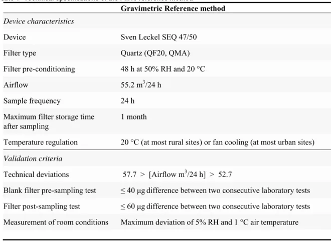
The reference method for PM10 measurements is the gravimetric method as described in the EN12341

standard (CEN, 1998). All reference measurements are carried out with a low volume sampler (LVS) conform to this standard. The technical specifications of the LVS used in this study are listed in Table 1. The LVS makes use of filters that are weighed before and after sampling. When the LVS is operating in the field, a constant airflow passes through this filter. Particles ≤ 10 μm are collected on this filter, and the filter is replaced at 24-h intervals. The daily average PM10 concentration is obtained

by calculating the difference in weight between the filters before and after sampling and then dividing the result by the airflow volume using the following equation

Equation (10). 10,DA DL B AF

F

F

PM

V

−

=

where PM10,DA is the daily average PM10 concentration measured in μg/m3, FDL is the dust-loaded

filter-weight after sampling (μg), FB is the blank filter-weight before sampling and VAF is the total volume of

the airflow used during the entire sampling period (m3/24 h) .

Two filter types have been used: QF20 and, more recently, QMA filters; both are quartz filters. The results of an experiment (details provided in Appendix B) reveal that there is no significant difference between the two filters in terms of PM10 concentrations, The analyses of the filters are carried out in an

air-conditioned weighing room maintained at the pre-prescribed conditions of 50% (±5%) RH and 20 °C (±1 °C). New filters are acclimatized at these conditions for at least 2 days prior to field usage, and the 24-h filters used in the field measurements are weighed under the same conditions. The samples are validated following the weighing process.

3.2

Validation

The gravimetric PM10 measurements are validated based on five conditions:

• All new filters are weighed twice before being used. The maximum allowed difference between the two measurements is 40 μg.

• The airflow during sampling is not allowed to deviate more than 2.5 m3 _{per 24-h period.}

• After sampling, all filters are weighed another two times. The difference between these two measurements cannot exceed 60 μg.

• The temperature and RH level in the weighing room is continuously monitored. If the RH or temperature deviates more than the maximum allowed variance (±5% RH and ±1 °C, respectively), then the sample in question will be rejected. However, until the beginning of 2006 the weighing room appears to have systematically operated at a RH below 45%. An experiment has been conducted to determine a correction factor for this deviation instead of all samples being rejected. See section 3.4.

• Remarks of individuals involved in the whole measurement process are considered during the validation process. For example, the result from a filter contaminated by parts of insects can be rejected during validation.

Table 1 Technical specifications of the PM10 reference method

Gravimetric Reference method Device characteristics

Device Sven Leckel SEQ 47/50 Filter type Quartz (QF20, QMA) Filter pre-conditioning 48 h at 50% RH and 20 °C Airflow 55.2 m3/24 h

Sample frequency 24 h Maximum filter storage time

after sampling

1 month

Temperature regulation 20 °C (at most rural sites) or fan cooling (at most urban sites)

Validation criteria

Technical deviations 57.7 > [Airflow m3/24 h] > 52.7

Blank filter pre-sampling test ≤ 40 μgdifference between two consecutive laboratory tests Filter post-sampling test ≤ 60 μgdifference between two consecutive laboratory tests Measurement of room conditions Maximum deviation of 5% RH and 1 °C air temperature

3.3

Comparability

The comparability of RM devices is described by the random uncertainty term, u2

(xi), which in the RM

used in this study is determined in a filter dependency experiment. In this experiment, a set of eleven RM devices are placed together, and equitability between different choices of filter material are examined together with the between-sampler uncertainty (see Appendix B). The results reveal a between-sampler uncertainty of 1.6 μg/m3_{, although lower between-sampler uncertainties have been}

obtained elsewhere; see, for example, the UK Equivalence Programme (Harrison et al., 2006). Another RIVM experiment that examined a possible difference between devices placed in open air and those inside an air-conditioned measurement room also obtained a smaller uncertainty (0.8 μg/m3). The

3.4

Correction of samples weighed at 43% relative humidity

Some of the RM samples have been analysed at an average RH of 43% due to shortcomings of the concerned device in the weighing room for a limited period of time. The European standard prescribes the RH to be 50% (±5%). Consequently, an experiment has been conducted to determine the effect of this deviation on the measurement results.

The change in filter mass can be examined either by increasing the RH from 43% to 50% or by decreasing it from 50% to 43%. However, hysteresis may occur when the RH is increased. In addition, the atmospheric RH in the Netherlands rarely reaches levels below 50%. Therefore, to mimic the field conditions as closely as possible, the experiment is performed by lowering the RH in the weighing room. A 40% RH was chosen for practical reasons. Assuming a linear relation, the result can then be interpolated to 43%.

The weight of the blank filter itself changes when it is acclimatized at different humidity levels. As this change has also to be accounted for when determining the effect on the final concentration, the

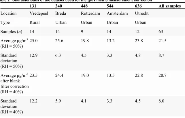
experiment is carried out in two steps. A sample set of 64 blank filters are first weighed, each filter individually, at 50% RH. The weighing room is then brought to 40% RH and the sample filters weighed a second time. The difference between the first and second measurements provides an estimate of the effect of weighing the blank filters at 40% RH instead of 50%. Second, a sample set of 63 filters are initially weighed at 50% RH and the filters placed into the field at five different locations (sites 131, 636, 240, 448 and 544). Table 2 lists the characteristics of each set of samples. After the appropriate sampling interval, the field sample filters are weighed at 50% RH and again at 40% RH. The difference between the first and second measurements provides an estimate of the effect of the deviating RH levels during weighing. Prior to determining the final correction factor, the effect on the blank filters is subtracted from the field samples. The final correcting factor is then computed using ordinary least square analysis, with the corrected field samples weighed at 40% RH as the dependant variable and the (uncorrected) field samples weighed at 50% RH as the independent variable (see Figure 1).

The result is a relative difference of –4.4% (R2 _{= 0.99) when the field samples are corrected with the}

offset found for the blank filters (–0.94 μg/m3) (see Figure 1). Assuming a linear relation, historic measurements weighed at 43% RH need to be corrected with a factor of 1.03 (100% + 4.4% × 0.7).

A contribution to the relative uncertainty has to be accounted for in corrected RM measurements included in the equivalence study. This contribution (u2

rm_c) to the relative measurement uncertainty is

defined in Eq. (11). Using this equation, the contribution is calculated to be 0.6 μg/m3 (0.83 μg/m3× 0.7). 2 2 _

(

)

2

x

y

u

n

−

=

∑

where xi and yi are the uncorrected and corrected RM measurements, respectively, used to determine

Table 2 Characteristics of the dataset used for the gravimetric measurement correction

131 240 448 544 636 All samples

Location Vredepeel Breda Rotterdam Amsterdam Utrecht Type Rural Urban Urban Urban Urban

Samples (n) 14 14 9 14 12 63 Average μg/m3 (RH = 50%) 25.0 25.6 19.8 13.2 23.8 21.5 Standard deviation (RH = 50%) 12.9 6.3 4.5 3.3 4.8 8.7 Average μg/m3 after blank filter correction (RH = 40%) 23.5 24.4 19.0 13.5 22.8 20.7 Standard deviation (RH = 40%) 12.2 5.9 4.1 3.3 4.5 8.0

Regression analysis for gravimetric PM₁₀measurements weighed at 40 % relative humidity

y = 0.96x R2 = 0.99 0 10 20 30 40 50 60 PM 10 μ g/ m 3 w ei ghed at 40% R H , cor rec ted f or bl ank fi lter of fs et

4

Candidate method

4.1

Characteristics

In the Dutch National Air Quality Monitoring Network (NAQMN), the number of automated PM10

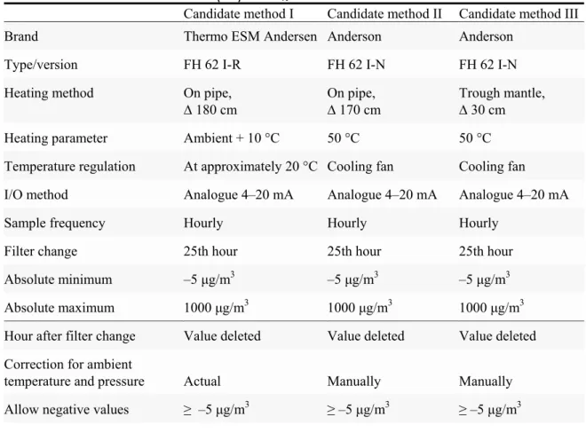
monitoring sites expanded from approximately 20 to 40 between 2003 and 2006. In 2006, roughly half of the monitoring sites were equipped with an old monitor model (FH62 I-N), while the other half were equipped with the newer model (FH62 I-R). All old models will be replaced with the new type in 2007 and 2008. The equivalence for both models is examined for consistency between historical

measurements. For technical details of each candidate method, see Table 3.

The heating system of the old model has in recent years been replaced by a new type of heating system due to discontinuance in the distribution of the old heating instrument. The method of heating has an important influence on the possible loss of volatile material. The new heating device is more than fivefold longer than the old one and, therefore, the two devices differ significantly (Table 3).

Consequently, a distinction is made between the FH 62 I-N model with an old heating system and that with the new one, thereby introducing a third candidate method.

Table 3 Overview of candidate methods (CM) for PM10 measurements in the Netherlands.

Candidate method I Candidate method II Candidate method III Brand Thermo ESM Andersen Anderson Anderson

Type/version FH 62 I-R FH 62 I-N FH 62 I-N Heating method On pipe,

∆ 180 cm

On pipe, ∆ 170 cm

Trough mantle, ∆ 30 cm Heating parameter Ambient + 10 °C 50 °C 50 °C Temperature regulation At approximately 20 °C Cooling fan Cooling fan I/O method Analogue 4–20 mA Analogue 4–20 mA Analogue 4–20 mA Sample frequency Hourly Hourly Hourly

Filter change 25th hour 25th hour 25th hour Absolute minimum –5 μg/m3 –5 μg/m3 –5 μg/m3 Absolute maximum 1000 μg/m3 _{1000 μg/m}3 _{1000 μg/m}3

Hour after filter change Value deleted Value deleted Value deleted Correction for ambient

temperature and pressure Actual Manually Manually Allow negative values ≥ –5 μg/m3 ≥ –5 μg/m3 ≥ –5 μg/m3

4.2

Validation

The automatic PM10 measurements (CM) are validated based on four criteria:

• Values below –5 μg/m3 _{are automatically rejected.}

• In the case of mechanical alerts and technical malfunctions, a signal of 2 mA is given by the monitor; these values are automatically rejected.

• A comparison with comparable monitoring stations and other measurements at the station are considered in order to determine a possible malfunctioning of the device.

• The first sample taken after each filter change is automatically rejected as this sample is typically different. The daily average concentration is based on the European Union’s criteria of a minimum of 13 validated samples per 24-h period (Guideline 2001/752/EC).

4.3

Comparability

Two experiments are carried out in which a between-sampler uncertainty is determined for the FH62-IR. In the first experiment, PM10 concentrations are measured with four parallel samplers for a

period of 19 days. Based on the results of this experiment, a between-sampler uncertainty of 0.76 μg/m3 is calculated (see Appendix D). In a second experiment, two samplers are placed together for

approximately 1 year. Based on the results of this experiment, a between-sampler uncertainty of 2.56 μg/m3 is calculated. Both determined uncertainties comply with the between-sampler limit as recommended by the EC Working Group (see also Appendix D).

4.4

Recalculation

The procedures, device configurations and settings in the NAQMN were checked thoroughly during the course of 2006 with the aim of improving the quality of the measurements and to prevent technical deviations from influencing the equivalence study. The observations have led to a revalidation of measurements and an improvement of procedures. The equivalence study is carried out using the revalidated data only. More information on the entire revalidation process can be found in the RIVM publication (in Dutch) of Beijk et al. (2007).

Historically, the old heating device (model FH62 I-N) was not equipped with an ambient temperature and pressure sensor. Prior to 2003 and, in some cases, up to 2005, particulate matter concentrations were therefore reported using standard conditions (20 °C, 1013 hPa). European legislation states that PM10 concentrations are to be based on prevailing atmospheric conditions. Consequently, historical

data are recalculated to meet this demand and to ensure consistency in trends. Neither atmospheric temperature nor pressure is simultaneously available with all PM10 measurements, and meteorological

data from the Dutch Royal Meteorological Institute (KNMI) are used to recalculate the PM10

measurements. Although the distance between KNMI stations and that between PM10 monitors may

where for each measured hour-average t, PM10 (μg/m3) concentrations are corrected with the ambient

and standard pressure (hPa) ratio and with the standard and environment temperature ratio (°C). The recalculation is further discussed and elucidated in a report by Berkhout et al. (2008).

5

Equivalence results

The results are given for the entire dataset of each CM, for a split dataset (samples higher than 50% of the European upper assessment threshold) and for each individual comparison (site). A possible calibration of a CM is based on the outcome for the entire dataset. Results of the split dataset and those of the individual sites illustrate the extent to which the results of the full CM dataset reflect prevailing field characteristics at the various locations.

5.1

Data characteristics

In total, 763 daily average samples at eight different sites are used for the comparison between the RM and the new (automatic) sampler at rural locations (CM-I rural). A total of 463 samples measured at four different sites comprises the dataset for urban sites (CM-I urban). Reference measurements for comparison with the old monitor model are only available at urban sites: 181 samples at two different sites for those with the original (static) heating device (CM-II) and 239 samples at two different sites for the old model with the new heating device (CM-III). The geographical position of each sampling sites is given in Figure 2. Outliers are not removed from any of the datasets during the analyses carried out in this study. The number of statistical outliers (samples outside the 99% confidence interval) are listed along with the results.

Candidate methods II and III are one and the same device. It was initially considered to treat these as one CM. However, the alteration in the inlet heating device leads to an important difference, and the dataset is therefore separated into two datasets. The consequence of separating the dataset is that the now following two candidate methods no longer comply with the recommended minimum number of comparisons. Both candidate methods are no longer technically supported and are replaced with a new type in the NAQMN. Despite the limited datasets the differences between CM-II and CM-III are considered to be of such magnitude that treating them separately would meet the field conditions better opposed to treating them as one.

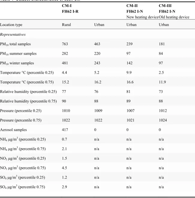
An overview of the characteristics and meteorological conditions of each CM is given in Table 4. The latter is given in percentiles to provide an impression of the distribution of prevailing meteorological conditions within each dataset. Where available, aerosol measurements are also presented (in percentiles).

5.2

Calibration and equivalence of the four candidate methods

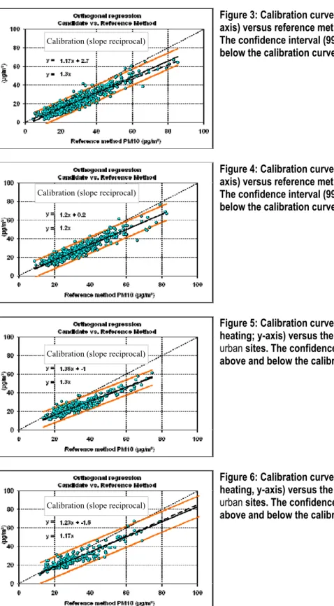
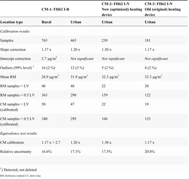
The regression results for the CM (full datasets) assessed here are shown in Figure 3 to Figure 6. The results for the new device (CM-I: FH62 I-R) at rural sites show a slope of 1.17, with a 2.7 μg/m3 offset; this is the only category with a statistical significant intercept. The relative (measurement) uncertainty for this category is 17%. Results for the same device but at urban sites present a slope of 1.20 based on orthogonal regression forced through the origin, with a relative uncertainty of 17%. Both sets of results comply with the European quality objective of 25% (see also Table 5 for the statistical results for each CM). The regression results for the old device (CM-II and CM-III; FH62 I-N new and old heating, respectively) at urban sites shows a slope of 1.30 and 1.20 for the configuration with the new and old

heating, respectively. The relative uncertainty of the former is 18%, and that of the latter is 21%. Consequently, both uncertainties are within the boundaries of the European quality objective of 25%.

Table 4 Dataset characteristics of each CM CM-I FH62 I-R

CM-II FH62 I-N

New heating device CM-III FH62 I-N Old heating device

Location type Rural Urban Urban Urban

Representatives PM10 total samples 763 463 239 181 PM10 summer samples 282 220 97 84 PM10 winter samples 481 243 142 97 Temperature °C (percentile 0.25) 4.4 5.2 9.9 2.5 Temperature °C (percentile 0.75) 15.2 16.2 16.6 11.9

Relative humidity (percentile 0.25) 77 76 81 73

Relative humidity (percentile 0.75) 90 88 89 88

Pressure (percentile 0.25) 1010 1009 1007 1012

Pressure (percentile 0.75) 1022 1022 1021 1024

Aerosol samples 417 0 0 0

NH4 μg/m3 (percentile 0.25) 0.7 n/a n/a n/a

NH4 μg/m3 (percentile 0.75) 2.1 n/a n/a n/a

NO3 μg/m3 (percentile 0.25) 1.5 n/a n/a n/a

NO3 μg/m3 (percentile 0.75) 4.5 n/a n/a n/a

SO4 μg/m3 (percentile 0.25) 1.2 n/a n/a n/a

SO4 μg/m3 (percentile 0.75) 2.9 n/a n/a n/a

Figure 3: Calibration curve for CM-I (FAG62-IR; y-axis) versus reference method (x-y-axis) at rural sites. The confidence interval (99%) is drawn above and below the calibration curve.

Figure 4: Calibration curve for CM-I (FAG62-IR, y-axis) versus reference method (x-y-axis) at urban sites. The confidence interval (99%) is drawn above and below the calibration curve.

Figure 5: Calibration curve for CM-II (FAG62-IN new heating; y-axis) versus the reference method at

urban sites. The confidence interval (99%) is drawn

above and below the calibration curve.

Figure 6: Calibration curve for CM-III (FAG62-IN old heating, y-axis) versus the reference method at

urban sites. The confidence interval (99%) is drawn

above and below the calibration curve. Calibration (slope reciprocal)

Calibration (slope reciprocal)

Calibration (slope reciprocal)

Table 5 Calibration and equivalence test results for each CM using the full datasets CM-1: FH62 I-R

CM-2: FH62 I-N New (optimized) heating device

CM-3: FH62 I-N Old (original) heating device

Location type Rural Urban Urban Urban

Calibration results

Samples 763 463 239 181

Slope correction 1.17 x 1.20 x 1.30 x 1.17 x

Intercept correction 2.7μg/m3

Not significant Not significant Not significant

Outliers (99% level) 1 _{16 (2 %) 12 (3 %) 5 (2 %) 4 (2 %)} Mean RM 26.9μg/m3 _31.9μg/m3 _32.3μg/m3 _32.3μg/m3 RM samples > LV 46 46 22 20 RM samples > 0.5 LV 363 298 159 122 CM samples > LV (calibrated) 50 47 22 19 CM samples > 0.5 LV (calibrated) 340 295 166 125

Equivalence test results

CM calibration 1.17 x + 2.7 1.20 x 1.30 x 1.17 x

Relative uncertainty 16.6% 17.1% 17.5% 20.8%

1_{) Detected, not deleted} RM, Reference method LV, limit value

5.3

Level of representativeness

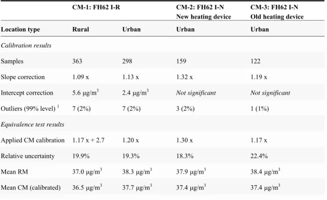
The results of the split datasets with only samples greater than 50% of the limit values are given in Table 6. Although the regression results differ slightly from those obtained with the full datasets, the resulting relative measurement uncertainty, which is calculated after the application of the appropriate CM calibration, remains beneath 25% for all split datasets

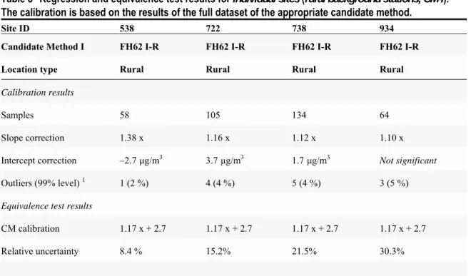
The results for each individual comparison (monitoring site) are given in Table 7 to Table 10. To determine the relative uncertainty of each comparison separately, each sub-dataset is calibrated by applying the earlier determined CM calibration – not by using the individual regression result. After the sub-datasets are calibrated, the results for all individual comparisons except one present a relative uncertainty that lies beneath the quality objective. Site 934 (Kollumerwaard, in the north of the Netherlands) presents a relative uncertainty of 29%, which is somewhat above the quality objective.

Table 6 Regression and equivalence test results using datasets with only samples greater than or equal to 50% of the limit value ( ≥ 25 μg/m3_{). Calibration is based on the results of the full dataset.}

CM-1: FH62 I-R CM-2: FH62 I-N

New heating device

CM-3: FH62 I-N Old heating device

Location type Rural Urban Urban Urban

Calibration results

Samples 363 298 159 122

Slope correction 1.09 x 1.13 x 1.32 x 1.19 x

Intercept correction 5.6μg/m3 _2.4μg/m3

Not significant Not significant

Outliers (99% level) 1 _{7 (2%) 7 (2%) 3 (2%) 1 (1%)}

Equivalence test results

Applied CM calibration 1.17 x + 2.7 1.20 x 1.30 x 1.17 x

Relative uncertainty 19.9% 19.3% 18.3% 22.4%

Mean RM 37.0μg/m3 _38.3μg/m3 _37.9μg/m3 _38.4μg/m3

Mean CM (calibrated) 36.5μg/m3 _37.7μg/m3 _37.4μg/m3 _37.4μg/m3

1_{) Detected, not deleted}

Table 7 Regression and equivalence test results for individual sites (rural background stations, CM-I). The calibration is based on the results of the full dataset of the appropriate candidate method.

Site ID 131 235 437 444

Candidate Method I FH62 I-R FH62 I-R FH62 I-R FH62 I-R

Location type Rural Rural Rural Rural

Calibration results

Samples 247 39 52 64

Slope correction 1.15 x 1.25 x 1.35 x 1.23 x

Intercept correction 5.8μg/m3 _1.6μg/m3 _{Not significant Not significant}

Outliers (99% level) 1 _{13 (5%) 0 (0%) 1 (2%) 1 (2%)}

Table 8 Regression and equivalence test results for individual sites (rural background stations, CM-I). The calibration is based on the results of the full dataset of the appropriate candidate method.

Site ID 538 722 738 934

Candidate Method I FH62 I-R FH62 I-R FH62 I-R FH62 I-R

Location type Rural Rural Rural Rural

Calibration results Samples 58 105 134 64 Slope correction 1.38 x 1.16 x 1.12 x 1.10 x Intercept correction –2.7μg/m3 _3.7μg/m3 _1.7μg/m3 Not significant Outliers (99% level) 1 _{1 (2 %) 4 (4 %) 5 (4 %) 3 (5 %)}

Equivalence test results

CM calibration 1.17 x + 2.7 1.17 x + 2.7 1.17 x + 2.7 1.17 x + 2.7

Relative uncertainty 8.4 % 15.2% 21.5% 30.3%

1_{) Detected, not deleted}

Table 9 Regression and equivalence test results for individual sites (urban stations, CM-I). The calibration is based on the results of the full dataset of the appropriate candidate method.

Site ID 240 433 448 641

Candidate Method I FH62 I-R FH62 I-R FH62 I-R FH62 I-R

Location type Urban Urban Urban Urban

Calibration results

Samples 69 67 248 79

Slope correction 1.36 x 1.25 x 1.20 x 1.18 x

Intercept correction Not significant Not significant Not significant Not significant

Outliers (99% level) 1 _{6 (9%) 2 (3%) 7 (3%) 2 (2%)}

Equivalence test results

CM calibration 1.20 x 1.20 x 1.20 x 1.20 x

Relative uncertainty 23.7 % 18.8 % 15.6 % 18.5 %

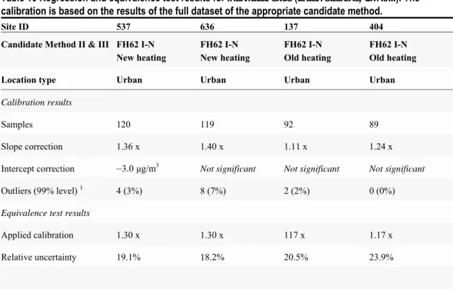
Table 10 Regression and equivalence test results for individual sites (urban stations, CM-II/III). The calibration is based on the results of the full dataset of the appropriate candidate method.

Site ID 537 636 137 404

Candidate Method II & III FH62 I-N New heating FH62 I-N New heating FH62 I-N Old heating FH62 I-N Old heating

Location type Urban Urban Urban Urban

Calibration results

Samples 120 119 92 89

Slope correction 1.36 x 1.40 x 1.11 x 1.24 x

Intercept correction –3.0μg/m3

Not significant Not significant Not significant

Outliers (99% level) 1 _{4 (3%) 8 (7%) 2 (2%) 0 (0%)}

Equivalence test results

Applied calibration 1.30 x 1.30 x 117 x 1.17 x

Relative uncertainty 19.1% 18.2% 20.5% 23.9%

5.4

Aerosols (ammonium nitrate)

Ammonium nitrate is assumed to be important as a volatile component of PM10. Due to the preheating

of the airflow in the sampler, this component may become lost before the actual measurement inside this unit actually takes place. This component may therefore influence the difference between the CM and the RM method with respect to the calibration term(s).

In a first attempt to study the effect of ammonium nitrate on the calibration, the dataset is split in two subsets: one in which the PM10 samples contain a high (≥ 15) percentage of ammonium nitrate and one

with a low (<15) percentage. Both of these data subsets comprise slightly more than 200 daily average samples, of which somewhat more than 25% are measured during the ‘summer’ half year (April–

September) at rural sites.

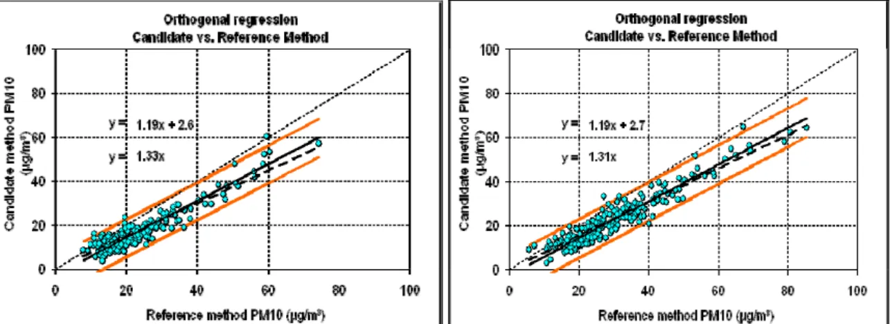
The resulting calibration curve for both datasets are illustrated in Figure 6. In both cases, the results are nearly identical: a slope of 1.19, with an intercept of approximately 2.6 μg/m3. The slope as well as the intercept are statistically significant for both datasets (twofold greater than its uncertainty). No clear relation between the level of ammonium nitrate and the calibration can currently be identified.

Figure 7: Calibration curve for the beta-gauge (FH62 I-R at rural sites) versus the reference method for samples with less than 15% ammonium nitrate (left) and those with ≥ 15% (right).

6

Conclusion

Outcome

The automatic PM10 measuring method (beta-attenuation) in the NAQMN is compared with the

European RM. Based on the results of this comparison, a calibration is introduced for four different configurations: the new model (FH62 I-R) at rural locations, the new model at urban locations, the old model (FH62 I-N) with a new heating system and the old model with an old heating system.

Equivalence is demonstrated for all four configurations after applying the assessed calibration. The resulting relative uncertainty for each CM varies between 16% and 21%. Following calibration of the CM measurements, fifteen of the sixteen locations included in this study comply with the European quality objective.

Where possible, a distinction is made between rural and urban locations. A sufficient number of parallel measurements are available for the new model to make this distinction. The old model,

however, is in the process of being replaced with the new model and is steadily being phased out of the NAQMN. Parallel reference measurements with the old model are limited to only urban locations; consequently, it is not possible to distinguish between urban and rural locations using this model. Although a comparison at rural locations is necessary to reconstruct a calibration for historical data, such a comparison is of little consequence for future PM10 measurements since the old model is phased

out of the monitoring network.

Definition of CM

The distinction between rural and urban locations raises a question relating to the definition of the CM. Two different beta-attenuation devices (old and new) are used in the NAQMN. The old model is physically modified through the replacement of the heating inlet system. While the monitoring device is basically the same, this modification might cause a difference in calibration. In addition, the same device at different locations is likely to lead to differences in calibration due to typical variations in particle composition – which is the reason underlying the EC Working Group’s recommendation for the test sites to be representative of ‘typical conditions’. However, there is currently no definition for determining whether or not a certain configuration is within the scope of these ‘typical conditions’. In this study, a CM is defined as a distinctive measuring device. Modification of the heating system leads to a device that is to be distinguishable from the original. Because of expected differences in composition between urban (both city background and street locations) and rural sites (background locations with possibly a larger fraction of secondary aerosols), a distinction is also made between the these two location types, leading to two subcategories.

Calibration method and regression forced trough the origin

Orthogonal regression is used for the determination of a possible calibration for each CM. Orthogonal regression without intercept is applied in the case of an insignificant intercept. The equations for orthogonal regression without intercept and corresponding uncertainty are not available in the

equivalence guideline. Such an approach was considered necessary; therefore, the statistical equations are presented and applied in this study.

Uncertainties

Conditions in the weighing room in which the RM samples are weighed appear to have deviated from the required 50% RH (±5%) up to 2006. This deviation has been corrected for, leading to a small contribution to the estimated relative uncertainty of the CM. This contribution is accounted for while testing equivalence. Another uncertainty that may have an effect when determining equivalence is the preconditioning of the RM filters. Although all filters are preconditioned for a minimum of 2 days – as prescribed in the CEN 12341 standard – dry filters may require a prolonged conditioning to reach an equilibrium. Currently applied procedures in the NAQMN have been modified so that all new filters reach their equilibrium before being used for sampling. Also, the weighing room has been completely modified and is ISO 17025 accredited. Both activities reduce uncertainties in current and future RM measurement results.

References

Beijk, R., Hoogerbrugge, R., Hafkenscheid, T.L., Arkel, F.Th. van, Stefess, G.C., Meulen, A. van der, Wesseling, J.P., Sauter, F.J., Albers, R.A.W. (2007) PM10: Validatie en equivalentie 2006 (in Dutch). Bilthoven: National Institute for Public Health and the Environment (RIVM). Report 680708001.

Berkhout, J.P.J., Mooibroek, D., Pul, W.A.J., Hoogerbrugge, R. (2008) Herberekening historische

meetgegevens fijnstof (in Dutch). Bilthoven: National Institute for Public Health and the

Environment (RIVM). Report 680708005.

CEN (1998) Air quality – Determination of the PM10 fraction of suspended particulate matter –

reference method and field test procedure to demonstrate reference equivalence of measurement methods. Brussels: CEN 12341.

EC Working Group on Guidance for the Demonstration of Equivalence (2005) Demonstration of

equivalence of ambient air monitoring methods. Published on the internet, February 28, 2007:

Available at: http://ec.europa.eu/environment/air/pdf/equivalence_report2.pdf.

EC (1996) Council directive 96/62/EC of 27 September 1996 on ambient quality assessment and

management. Official journal L 296, 21/11/1996 p. 0055-0063.

EC (1999) Council Directive 1999/30/EC of 22 April 1999 relating to limit values for sulphur dioxide,

nitrogen dioxide and oxides of nitrogen, particulate matter and lead in ambient air. Official

Journal L 163: 29/06/1999 p. 0041 – 0060.

Harrison, D., Maggs, R., Booker, J. (2006) UK Equivalence Programme for Monitoring of Particulate

Matter. Bureau Veritas, Report Reference BV/AQ/AD202209/DH/2396.

Isobe, T., Feigelson, E.D., Akriteas, M.G., Babu, G.J. (1990) Linear regression in Astronomy. Astrophysical Journal, vol. 364, pp. 104-113

WHO (2004) Health aspects of air pollution. Results from the WHO project “Systematic review of

health aspects of air pollution in Europe”. European centre for Environment and Health –

Bonn Office. Denmark: World Health Organization Europe. Publication E83080. WHO (2005) Effects of air pollution on children’s health and development. A review of evidence.

European centre for Environment and Health – Bonn Office. Denmark: World Health Organization Europe, Publication E86575.

WHO (2006) Health risk of particulate matter from long-range transboundary air pollution. Joint WHO/Convention Task Force on the health aspects of air pollution. Denmark: World Health Organization Europe, Publication E88189.

Appendix A: Orthogonal regression

Derivation of the slope parameter in orthogonal regression with zero intercept

In this section a derivation for the slope coefficient and associated standard error is given. We will use the least squares principle and minimize the sum of the squared perpendicular distances

d

y

ˆ

=

a

+

b

x

ˆ

The horizontal distance from a point to the line is hi = xi −

xˆ

yˆ

According to Pythagoras' law

h

v

the area of the big triangle, so di(pi + qi) = hivi. Combining these two equations and solving for di, we

find: 2 2 i i i i i

v

h

v

h

d

+

=

Using the above equations, this can be written in terms of xi, yi, a and b:

2

1 b

bx

a

y

d

+

−

−

=

As in regular linear regression, where the vertical distances, or residuals, vi are assumed to be normally

distributed with zero expectation and a common variance, we may also assume that the perpendicular distances di are normally distributed with zero expectation and a common variance σ2. Using maximum

likelihood theory, we can now derive orthogonal regression expressions for both a and b and their standard errors. Because we wish to derive an expression for the slope b only, we set a = 0. The likelihood function for one observation then becomes:

⎟⎟

⎠

⎞

⎜⎜

⎝

⎛

+

−

−

=

)

1

(

2

)

(

exp

2

1

)

,

|

,

(

σ

πσ

σ

b

bx

y

b

y

x

f

)

ˆ

,

ˆ

(

x

y

)

ˆ

,

(

x

y

)

,

(

x

y

)

,

ˆ

(

x

y

The likelihood for n independent observations is the product n times the above expression. This function is maximized. The log is usually taken first, so the log-likelihood for n observations becomes:

∑

+

−

−

−

=

b

bx

y

n

b

y

x

f

)

1

(

2

)

(

)

2

log(

2

)]

,

|

,

(

log[

σ

πσ

σ

which can be written as:

2 2 2 2 2

)

1

(

2

2

)

2

log(

2

)]

,

|

,

(

log[

σ

πσ

σ

b

Sxx

b

bSxy

Syy

n

b

y

x

f

+

+

−

−

−

=

In the above equation,

∑

=

=

x

Sxx

∑

=

y

Syy

∑

=

y

x

Sxy

. In order to find the maximum, we calculate the partial derivatives of the above equation with respect to b and σ2. These should be equal to zero. After a little simplification, we find:

0

)

1

(

2

)

1

(

)]

,

|

,

(

log[

=

+

+

−

+

+

−

=

∂

∂

σ

σ

σ

b

Sxx

b

bSxy

Syy

b

b

bSxx

Sxy

b

b

y

x

f

0

)

1

(

2

2

2

)]

,

|

,

(

log[

=

+

+

−

+

−

=

∂

∂

σ

σ

σ

σ

b

Sxx

b

bSxy

Syy

n

b

y

x

f

The first equation is solved for b. This appears to be a quadratic equation with two solutions. After a rearrangement of terms, the expression for the slope parameter we are interested in is:

Sxy

Sxy

Sxx

Syy

Sxx

Syy

b

2

4

)

(

₋

₊

+

−

=

The second equation is solved for σ2. After a rearrangement of terms, the expression for the residual variance is:

)

1

(

2

b

n

Sxx

b

bSxy

Syy

+

+

−

=

σ

The next step is the derivation of the standard error of b. In maximum likelihood theory, this is achieved by calculating the inverse Hessian minus the log-likelihood function. The variances of the parameters are then along the diagonal. However, since we are only interested in the standard error of

b, we can substitute the expression for the residual variance minus the log-likelihood function and

simply take the reciprocal of the second order derivative with respect to b. This is then equal to var(b). After substituting σ2 in the log-likelihood function and some simplification, the minus log-likelihood function becomes:

⎥

⎦

⎤

⎢

⎣

⎡

+

−

+

+

−

−

−

+

=

∂

−

∂

)

1

(

1

)

2

(

2

)

2

(

)]

|

,

(

log[

b

b

Sxx

b

bSxy

Syy

Sxy

Sxx

Sxx

b

bSxy

Syy

n

b

b

y

x

f

Finally, var(b) is the reciprocal of the above expression:

=

)

var(b

)

1

(

1

)

2

(

2

)

2

(

1

⎥

⎦

⎤

⎢

⎣

⎡

+

−

+

+

−

−

−

+

b

b

Sxx

b

bSxy

Syy

Sxy

Sxx

Sxx

b

bSxy

Syy

n

The standard error of b is the square root of the variance of b.

Comparison and validation

The standard error of the orthogonal fit forced through the origin is calculated for each of the candidate methods (CM) defined in this study with no statistical significant intercept as well as for three random individual sites and one small random dataset. The results for three different methods are presented in the table below. The first, u(b), is based on the formulae given in Appendix B of the equivalence guideline with the modification described in section 2.2, the second, u(b)maxlike, is based on the

maximum likelihood method as described in Appendix A, and the third is based on the bootstrap method (non-analytical). The results for all three are nearly identical. Only in the case of a very small number of samples may a minor difference occur (e.g. a few thousandths μg/m3). The largest observed difference between the two analytical methods is approximately 0.0012 μg/m3 _(5%).

Based on these results it is concluded that all three methods provide fairly similar results, although minor differences of less than 0.001 may occur. These differences are negligible in the determination of the relative combined uncertainty within the scope of this equivalence study. Therefore, the least complicated method (modified version of the equations given by the EC Working Group) is used for this study, while still taking into consideration the usability of possible future adaptations in a revision of the Working Group’s guideline.

Table A1 Regression coefficient standard uncertainties (forced trough origin) using different methods

Category n Sxx Syy Sxy b u(b)* u(b)maxlike** u(b)bootstrap***

FH62 IR Urban 463 546838 378801 451219 0.83 0.00507 0.00509 0.00626 FH62 IN New heating Urban 239 284798 169323 217588 0.77 0.00675 0.00676 0.00707 FH62 IN Old heating Urban 181 225082 165021 190411 0.85 0.00986 0.00991 0.011150 Random1 12 2907 1496 2069 0.72 0.02739 0.02632 0.027130 Site 131 247 239351 119139 166758 0.70 0.00709 0.00711 0.008927 Site 235 39 42500 24475 32122 0.76 0.01106 0.01093 0.011914 Site 934 64 39561 32637 35741 0.91 0.01180 0.01175 0.015355

1 _{Small random dataset (n=12) with an average of 15 μg/m}3_.

* _{Standard error calculated with the modified equations as demonstrated in section 2.2.} ** _{Standard error calculated with the maximum likelihood method.}