Existing data and knowledge gaps about air-climate inter-linkages and way forwards for improvement

(1)

Existing data and knowledge gaps about

air-climate inter-linkages

and way forwards for improvement

ETC/ACM Technical Paper 2014/7

March 2015

Augustin Colette, Jelle van Minnen, Hans Eerens,

Paul Ruyssenaars, Jeroen Peters, Benno Jimmink,

Frank De Leeuw, Laurence Rouïl

The European Topic Centre on Air Pollution and Climate Change Mitigation (ETC/ACM) is a consortium of European institutes under contract of the European Environment Agency RIVM Aether CHMI CSIC EMISIA INERIS NILU ÖKO-Institut ÖKO-Recherche PBL UAB UBA-V VITO 4Sfera

(2)

Front page picture

Typology of aerosol dominating the PM10 mix (pink: primary anthropogenic, green: secondary, blue: sea-salt, brown: desert dust) modelled by INERIS with the CHIMERE model for the winter of 2009. This picture highlights the need to account for the secondary fraction of aerosol when deriving impacts from primary emission projections.

Author affiliation

A. Colette, L. Rouïl: Institut National de l'Environnement Industriel et des Risques (INERIS), France J.G van Minnen, H.C. Eerens, J. Peters: Planbureau voor de Leefomgeving (PBL), the Netherlands

B. Jimmink, P. Ruyssenaars, F. de Leeuw: Rijksinstituut voor Volksgezondheid en Milieu (RIVM), the Netherlands

DISCLAIMER

© ETC/ACM, 2014.

ETC/ACM Technical Paper 2014/7

European Topic Centre on Air Pollution and Climate Change Mitigation PO Box 1 3720 BA Bilthoven The Netherlands Phone +31 30 2748562 Fax +31 30 2744433 Email etcacm@rivm.nl Website http://acm.eionet.europa.eu/

This ETC/ACM Technical Paper has not been subjected to European Environment Agency (EEA) member country review. It does not represent the formal views of the EEA.

(3)

1 Introduction

1.1 Scope

The knowledge base on air-climate interactions is growing, especially with increasing interest created by activities of the IPCC, IGBP/IGAC, EU research projects and the recognition of the role of short lived climate forcers under LRTAP and the UNEP BC assessment, development of a 2030 framework for EU climate and energy policies, and not to forget activities under the former ETC/ACM consortium (2010-2013). It is therefore important that EEA maintains and expands its understanding of the drivers of atmospheric change, their interaction, and the resulting changes in atmospheric composition, as well as their impact on human health and ecosystems in order to share this information with the EEA member countries and the European Union institutes.

Figure 1: Schematic diagram of the impact of air pollution emission controls and climate impacts. Solid black lines

indicates known impacts, dashed lines indicates uncertain impacts (IPCC AR5, Chapter 8, FAQ 8.2)

Over the past years progress has been made in understanding the linkage between air pollution with climate change (Figure 1). For example, it became clear how air pollutants contribute to climate forcing (enhancing or decreasing it) and how they affect precipitation patterns through indirect radiative forcing (IPCC, 2013). Koren et al (2014) have recently shown that even small amounts of aerosols can affect the number and size of clouds. At the same time climate change can lead to changing distribution patterns of air pollutants (Jacob and Winner, 2009), and reforestation (often seen as a climate change mitigation measure) can be a cost-effective abatement measure for ground-level ozone and nitrogen oxide (Kroeger et al, 2014). And we need to keep in mind that reductions in air pollutants/SLCPs can delay global warming and as such be useful to help society and environment to adapt to climate change. But it cannot prevent a substantially greater warming in the longer term. In other words, reducing the emissions of CO2 and other well-mixed GHGs remains needed to keep the global temperature increase within the 2°C target (see also Solomon et al, 2013).

Using data available from, and in collaboration with, current integrated assessment models and activities such as GAINS (IIASA), FASST (JRC), IMAGE (PBL), and results from EU research projects (e.g. Pegasos) and ETC/ACM studies, the purpose of the present document is to identify the main data

and knowledge gaps on air-climate interlinkages and propose how to close this information gap in the coming years through collaboration activities and future targeted assessment studies.

This with a focus on information concerning Europe and the EEA member countries and on the following three topics:

(5)

(i) Emission scenarios: completeness of scenarios in terms of coverage of both air pollutants and greenhouse gases and availability of AP and GHG scenarios that consider a variation of climate change policies, both for the time frame present day-2050.

(ii) Climate impact: support the decision on the most appropriate indicator (RF, ERF, GTP or GWP, absolute or relative) and secure availability of the relevant indicator for all compounds at the geographical and temporal scale selected.

(iii) Health and ecosystems impacts: Unlike climate impacts, there are no simple transfer function that can provide impacts of a given emission reduction measure. The only options are (1) emission response models (FASST, GAINS, SNAP) or (2) full frame chemistry transport models. A review of the strengths and weaknesses of each approach will be performed including assessment of availability of the models, required input data and expected outcomes in terms of health and ecosystem impacts.

While the section on emission scenarios (2) will put and emphasis on the synergies between air quality and climate measures, the subsequent sections (3 on climate impacts and 4 on health & ecosystems) will be focused on either one or the other.

1.2 State of the art

Assessing the combined impacts of various social and economical projections or environmental policies on climate and air quality is classically referred to as integrated assessment modelling. Suite of models (see Annex I for short descriptions of such models) are used to develop scenario and assess multiple impacts, some examples:

- Social-economic models that are used to provide the input for the demographical and economic changes foreseen. Some examples are GEM-E3, Worldscan, MERGE, Witch, ENV-linkages.

- Sectoral models such as TREMOVE (transport sector), CAPRI, MAGNET (Agricultural sector), PRIMES (energy sector) and/or specific model such as GTAP (international trade).

- Models that are used to generate emissions from the economic activities, some examples are POLES, PRIMES, GAINS, TIMER.

- Models that are used to calculate concentrations/impact from the estimated emissions, these models include chemistry transport models such as TM5, EMEP, CHIMERE, or surrogate models such as FASST, IMAGE, GAINS.

- Models that are used to calculate the change in climatic parameters due to a change of GHG and air pollutant concentration, i.e. global coupled general circulation models (Hadley, IPSL, ECHAM). - A few models are integrated over the whole chain; examples for these types of models are GAINS

and IMAGE.

Models differ in spatial and temporal scales considered, and in the complexity of the simulation undertaken. Complexity can differ in number of economic sectors handled, spatial resolution, time horizon, emissions, impact calculated and technology (options) available. For models focusing on just one of the component of the chain listed above, feedbacks are often a weak point.

Introducing stringent measures in a certain sector or region will have an economic impact and create structural changes. When, for example, an energy tax is increased, the consumer will be motivated to invest in energy-saving options (through substitution or behavioural changes) as a result, the share of energy use in our economic system will be reduced. The more complex scenarios use a series of models to estimate the parameters including sensitivity runs or ensemble means of a series of comparable models (Figure 2).

(6)

Figure 2: Suite of models describing the DPSIR chain for the TSAP scenarios (IIASA, 2014).

Integrated Assessment Modelling is a complex topic that has been the focus of substantial scientific work in the past couple of decades. If some of the existing tools already offer the possibility to assess air and climate interlinkages, others are limited to a few (emission related) indicators. The present

report will review the capacities of available tools to assess the air climate interlinkages. In order to point out possible ways forward we will emphasise if bottlenecks can be attributed to current knowledge gaps or missing input data.

(7)

2 Emission scenarios

Emission scenarios classically include two components: a representation of a reference situation (that can be an actual emission inventory reported for a recent period) and a quantification of possible or plausible future pathways. These two components are introduced in the two subsections of the present chapter.

2.1 Emission projections

In this report a number of scenarios and models have been selected to assess the current state of play in climate-change-air quality inter linkages. In the next paragraph (2.1.1) the selection criteria that have been applied in selecting these scenarios are presented. In paragraph 2.1.2 the selected scenarios are presented in order to point out some general notes on the state of play and possible improvement in the representation air-climate inter linkages at the end of this chapter (2.3.1). 2.1.1

Selection of scenarios

An initial set of criteria was developed and tested through a number of interviews with ETC/ACM experts in the field of air and climate (see interviews in Annex 1). The scenarios to be selected comply with most of the following requirements:

1. Have link with climate change and air quality policies; 2. Be recent (preferably developed after 2010);

3. Include different policy/decision making levels (EU, OECD, National );

4. Include a scenario with a focus on air quality strategies with climate change baseline and a scenario with a focus on climate change polices with air quality baseline;

5. Include a scenario focussing on European countries and a scenario focussing on the EU as part of a global assessment;

6. GHG and AP emissions should be available in the scenarios;

7. Beside End-of-Pipe (EOP) and CO2 reduction options, some scenarios should also include measures of the type that involve structural changes, consumer behaviour, energy/transport designs, food systems, etc.

8. Include wide ranging of scenarios (baseline, extreme/exploration, business as usual /current/best policies) that include an own story line, economic-social trend developments and various variants.

Taking note of the above given criteria, in the ETC/ACM expert’s opinion, the most important scenarios to consider were TSAP (from an air quality, European perspective) and the RCP scenarios (from a climate, global perspective, including follow-up studies such as EC-LIMITS, ECLIPSE, PEGASOS, CCMI, IC-IMAGES). The present report will focus on these two priority scenarios although there are possible additional scenarios that could comply with the selection criteria listed above. The Global Energy Assessment has developed energy projection pathways that comply with the RCP storylines and take into account air pollution policies, including a quantification of the associated costs. A scenario that studied especially economic interactions and could be of interest as an economic background scenario is the long-term growth scenario (up to 2060) from the OECD (OECD, 2013). Other scenario that were mentioned, but not yet fully reported is UNEP that prepares a new scenario based on GEO-5 with as important new aspects the flow of materials and more focused on LCA contributions. The models used to develop such scenarios, and possible alternative tools are presented in Annex II.

2.1.2

Short description of the TSAP and RCP scenarios.

2.1.2.1 TSAP scenario

The Thematic Strategy on Air Pollution (TSAP) –established in 2005- has been revised multiple times over recent years (see details http://gains.iiasa.ac.at/TSAP). The overall objective, however, remained the same, i.e. to explore how the European Union could make further progress in achieving levels of air quality that do not give rise to significant negative impacts on, and risks to human health

(8)

and environment’ (EEA, 2013, IIASA, 2013). All detailed data of the TSAP scenarios can be retrieved from the GAINS-online model (http://gains.iiasa.ac.at/gains/EUN/index.login?logout=1). The final TSAP 2013 Baseline employs the projection of economic activities (e.g., energy use, transport, agricultural production, etc.) that has been developed for the Commission Communication on ‘A policy framework for climate and energy in the period from 2020 to 2030’ (EC 2014a). It includes PRIMES2013 Reference Energy scenario. The CAPRI model has been used to project future agricultural activities in Europe consistently with the macro-economic assumptions of the PRIMES-2013 Reference scenario and considering the likely impacts of the most recent agricultural policies.

The following GHG emissions are available in the GAINS-online tool: CO2, CH4, N2O and F-gases. For CO2, regulations are included in the PRIMES calculations as they affect the structure and volumes of energy consumption. For non-CO2 greenhouse gases and air pollutants, EU and Member States have issued a wide body of legislation that limits emissions from specific sources, or have indirect impacts on emissions through affecting activity rates. The effect of these legislations have been assessed through bilateral consultations with the EU member states. For the Commission proposal on the Clean Air Policy package the current legislation for CH4 emissions that is assumed in the GAINS baseline projection is used.

The following air pollutant emissions are available in TSAP: SO2, NOx, PM2.5, NH3, VOC, BC, OC, TSP. In order to explore future European air quality, the TSAP emissions scenarios needs to be refined. In particular, the data must be distributed on a spatial grid and available for a minimum set of chemical species (pollutants and their precursors). The TSAP emission data were therefore further processed, to allow air quality modelling, in the Eclipse FP71_{project. They were delivered in May 2013. A more} detailed review of the ECLIPSE scenario can be found in EEA, 2013b.

2.1.2.2 RCP scenarios

To support the assessment of the IPCC report various sets of scenarios have been developed over time (IPCC, 2013). The most recent are called the RCP (representative concentration pathways) scenarios. (Moss et al., 2010; Van Vuuren et al., 2011a). These scenarios form the basis of the current generation of climate model runs as part of the Atmospheric Chemistry and Climate Model Intercomparison Project (ACCMIP, Lamarque et al., 2013) and Coupled Model Intercomparison Project (CMIP5, Taylor et al., 2012). The RCP set consists of four scenarios (RCP2.6, RCP4.5, RCP6.0 and RCP8.5) each of which describes a different trajectory for emissions of long-lived greenhouse gases (LLGHGs) and short-lived air pollutants, the corresponding concentration levels, land use and radiative forcing. Together the four RCPs span a range of possible climate forcings varying from 2.6 W/m2_{to 8.5 W/m}2_{in 2100 (Van Vuuren et al., 2011a). It should be noted that the four RCPs have} been produced by four different (see Table 1) integrated assessment models (see Masui et al., 2011; Riahi et al., 2011; Thomson et al., 2011; Van Vuuren et al., 2011b, Colette et al., 2012).

For Europe, the RCP2.6 and 4.5 scenario’s leads to an almost 80% and 20% reduction of GHG emissions by 2050, while in the RCP6.0 and RCP8.5 scenarios the GHG emissions actually increase for Europe. The emissions trajectories of air pollutants are determined by three important factors: the level of economic activities, the assumed degree of air pollution control and the assumed level of climate policy (Van Vuuren et al., 2011a). In the RCPs, all modelling teams assumed that higher income levels lead to the implementation of more stringent air pollution control measures. Overall, this implies that in each RCP air pollutant emission factors gradually decline during the course of the century. In the Representative Concentration Pathways (RCP) database (RCP Database, 2009), emissions concentrations and land-cover change projections and radiative forcing are documented. Information on individual RCPs (RCP2.6, RCP 4.5, RCP 6.0 and RCP 8.5, see Table 1) is provided. Version 2.0 of the database includes harmonized and consolidated data for three of the four RCPs (RCP, 2009). Results of the model runs can be compared by using the RCP webtool. Sectoral 1_{http://eclipse.nilu.no/}

(9)

emissions for greenhouse gases and air pollutants2_{are available on a global regional scale for the} period 2000 – 2100 and also gridded information (0.5 x 0.5 global grid) is provided.

Table 1: Overview of models used in the development of RCP scenarios.

RCP Organisation Model

2.6 PBL Netherlands environmental Assessment Agency IMAGE

4.5 Northwest National Laboratory's Joint Global Change Research Institute

(JGCRI) MiniCAM

6.0 National Institute for Environmental Studies (NIES), Japan AIM

8.5 Integrated Assessment Framework at the International Institute for Applies

Systems Analysis (IIASA), Austria MESSAGE

The RCP scenarios were subsequently combined with 5 SSP scenarios3_{with different socio-economic} characteristics (see also Table 2):

– SSP1: Sustainable dev. world (env. tech, good governance, low population, wealthy, social/env goals important)

– SSP2: Medium

– SSP3: Fragmented world (regional competition, low tech., little trade, poor) – SSP4: Fragmentation in regions (strong rich/poor divide, poor on average)

– SSP5: High economic growth (strong technology, fossil fuel driven, consumption, human development).

Table 2: Main characteristics of the RCP/SSP scenarios (van Vuuren et.al.,2014).

2.1.3

Comparison of available projections

In Figure 3 the TSAP and RCP scenario’s are placed in a matrix with one axe (Y-axis) differentiating in Air Quality policies and the other (X-axis) differentiating in Climate Change policies. For TSAP two contrasting scenarios for Air Quality policies are presented (Current legislation and Maximum feasible reduction) but, no differentiation in Climate Change policies has been applied. For the RCP scenario there is a differentiation in as well Climate Change Policies as in Air Quality policies. Looking to the spatial resolution we see that the TSAP scenario’s show a relative high spatial resolution (Country level), while the RCP scenario is limited to the EU as a region.

2_{CO2, CH4, N2O, HFC, PFC, SF6, ODS, SO2, BC, OC, NOx, VOC and NH3.}

3_{The SSP scenarios can be viewed/download at:}_{https://secure.iiasa.ac.at/web-apps/ene/SspDb}

(10)

Figure 3: main characteristics in terms of adopted air pollution and climate change control policies

Another challenge to be overcome regards the fact that various scenarios may lack information on the compounds of interest to address air quality and climate interlinkages beyond emissions. For instance, even if RCP include air pollutant emission projections, they were designed primarily for the purpose of large scale chemistry and climate interactions rather than surface air quality assessments, providing insufficient information to allow air quality modelling of air pollutant levels at ground level and their impacts on human health and ecosystems (Colette et al., 2012; Fiore et al., 2012). To overcome the problem of insufficient air pollution information in the RCP scenario’s some additional work has been undertaken in new projects such as EC-IMAGE, LIMITS and PEGASOS (Chuwah et. Al, 2013, Braspenning-Radu at al, 2014). In the context of the PEGASOS project, a set of long-term scenarios that are relevant for both climate and air pollution research have been developed (Radu at al, 2012, 2014). They are consistent the RCP scenario’s and have additional, detailed, information about air pollutions. Using the derived Emission Factors (EF) for 2030, a set of 10 scenarios was developed by PBL until up to 2100.

For the air pollution policy scenario’s the following variants were developed (with 2005 as base year): 1. No improvement of policies after 2005, resulting in frozen emission factors (FRZ).

2. Current policies implemented up to 2030 and constant from 2030 onwards (CLE).

3. Further tightening of CLE after 2030 based on assumptions regarding economic development (CLE KZN).

4. Implementation of maximum feasible reductions until 2030, and constant from 2030 onwards (MFR).

5. MFR with further improvement after 2030 (MFR KZN).

These 5 future air pollution scenarios were combined with 2 sets of climate RCP scenarios (representing 2 radiative forcing targets in 2100: 2.6W/m² and 6W/m²). Table 3 presents the set of emissions delivered to PEGASOS and is available via http://www.eccad.fr

spatial resolution spatial resolution spatial resolution spatial resolution EU-Country EU-Region EU-Country EU-Region

TSAP_MFR RCP6.0/KZN RCP2.6/KZN

High OECD-BL/CLE-KZN RCP2.6/CLE-KZN

OECD-BL/MFR RCP2.6/MFR

OECD-BL/CLE + progress RCP2./CLE + progress

TSAP_CLE RCP6.0/Frozen RCP2.6/Frozen

OECD-BL/Frozen RCP2.6/Frozen

Low OECD-BL/CLE - 2030 Frozen RCP2.6/CLE - 2030 Frozen

OECD-BL/Frozen RCP2.6/Frozen

Low High

Climate policy Air pollution policy

(11)

Table 3: Overview of emission datasets produced within the PEGASOS4_{FP7 project.}

PEGASOS

Emission sources Antropogenic sources

Pollutants CH4, CO, NOx, NMVOC, SO2, NH3, BC, OC,

CO2, N2O

Temporal distribution Historical part: 1970-2005

Scenarios until 2100

Spatial distribution Downscaled to 0.5° x 0.5°

2.2 Emission inventories

This section reviews the main issues to be considered when assessing emissions inventories for the present day. As the emissions are an important input variable for modelling/scenario exercises, it’s important to take into account :

(1) Comparability of available emission inventories as basis for modelling; (2) Uncertainties in emission inventories;

(3) Available exercises for gridding of emissions that could be used as input for a more detailed/gridded approach for the metrics.

The main messages from this short analysis, is that the comparability & uncertainties of datasets should be considered when used for downscaling to a higher resolution; especially when we look at (increasingly important) issues like shipping and aviation.

2.2.1

Consistency across inventories

In this section the pollutants usually presented in scenario studies and reported in climate change and air pollutant emissions inventories are discussed, including the differences between the (sectoral) split of the pollutants, and their spatial resolution.

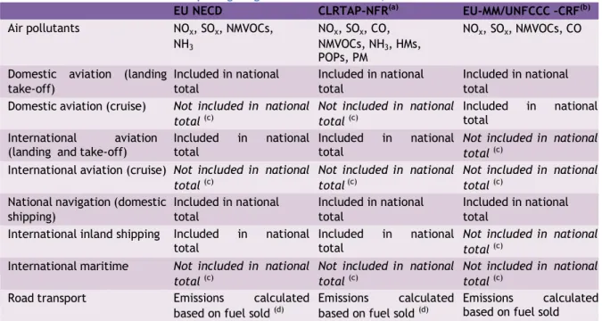
EU Member States report their emissions of SO2, NOx, NMVOCs and NH3 under the NEC Directive on national emission ceilings for certain atmospheric pollutants (EC, 2001), and emissions of NOx, CO, NMVOCs and SO2 under the EU Greenhouse Gas Monitoring Mechanism (EC, 2004). This information should also be copied by Member States to the EEA’s Eionet Reportnet Central Data Repository (CDR). The three reporting obligations differ in the number and type of air pollutants, the geographical coverage of Parties (for example the inclusion (or not) of overseas dependencies and territories of France, Spain, Portugal and the UK) and the inclusion of domestic and international aviation and navigation in the national total, but for most Parties the differences are only minor. The CLRTAP and NECD reporting formats are identical, CLRTAP and UNFCCC emission inventories differ slightly in the sector split (Table 4).

4_{ftp-ccu.jrc.it/pub/dentener/PEGASOS_WP14/VersionJanuary2014/PEGASOS_DELIVERABLE%2014_1-v1.doc.}

(12)

Table 4: Main differences between the reporting obligations under the CLRTAP, NECD and the UNFCCC.

EU NECD CLRTAP-NFR(a) _{EU-MM/UNFCCC –CRF}(b)

Air pollutants NOx, SOx, NMVOCs, NOx, SOx, CO, NOx, SOx, NMVOCs, CO

NH3 NMVOCs, NH3, HMs,

POPs, PM

Domestic aviation (landing Included in national Included in national Included in national

take-off) total total total

Domestic aviation (cruise) Not included in national

total (c) Not included in national _total(c) Included _total in national

International aviation

(landing and take-off) Included total in national Included total in national Not included in national total (c)

International aviation (cruise) Not included in national

total (c) Not included in national _total(c) Not included in national _total(c)

National navigation (domestic Included in national Included in national Included in national

shipping) total total total

International inland shipping Included in national

total Included total in national Not included in national total (c)

International maritime Not included in national

total (c) Not included in national _total(c) Not included in national _total(c)

Road transport Emissions calculated

based on fuel sold (d) Emissions _{based on fuel sold}calculated (d) Emissions _{based on fuel sold}calculated Note:

(a) _{‘NFR’ denotes ‘nomenclature for reporting’, a sectoral classification system developed by UNECE/EMEP for} reporting air emissions.

(b) _{‘CRF’ is the sectoral classification system developed by UNFCCC for reporting of greenhouse gases.} (c) _{Categories not included in national totals should still be reported by Parties as so-called ‘memo items’.} (d) _{In addition, Parties may report emission estimates on a fuel consumed basis as a ‘memo’ item.}

2.2.2

The specificity of international air and sea traffic

International Shipping5_{: Emissions from fuels used by vessels of all flags that are engaged in} international water-borne navigation. The international navigation may take place at sea, on inland lakes and waterways and in coastal waters. The definition includes emissions from journeys that depart in one country and arrive in a different country and excludes consumption by fishing vessels. International Aviation: Emissions from flights that depart in one country and arrive in a different country. Include take-offs and landings for these flight stages. Emissions from international military aviation can be included provided that the same definitional distinction is applied.

Emissions from International Shipping have been compared in an assessment published by EEA in 2013 (EEA Technical Report 2013/4, “The impact of international shipping on European air quality

and climate forcing”), showing that the contribution of international shipping to concentrations of

e.g. NO2 and PM2.5 in coastal areas is substantive (e.g varying between 5% and 20% along different European coasts for PM2.5).At the same time, the report concludes that there is a strong need for further harmonisation of emissions information from the shipping sector across Europe. The study found that a relative large share of GHG and air pollutants emissions from international shipping is not accounted for in national inventories supporting key conventions.

An unpublished overview (EEA, results of task 1.1.1.9 in 2014 by ETC/ACM) of reported International Aviation data by EU-28 countries compared to Eurostat data, shows large differences between (reported) datasets.

As to allow for further assessment activities, the quality of reported data should be improved – especially in the context of the increasing relative share of international sea traffic and aviation in total emissions

5_{The definitions apply to the present Guidelines and are taken from chapters 3.5.1 and 3.6.1 of volume 2 of the} IPCC Guidelines (IPCC, 2006).

(13)

2.2.3

Spatial resolution and geographical target areas.

Especially for air pollution impact studies the spatial resolution and characteristics (height, variation over the year, temperature) of the emitted pollutant is important in order to calculate the exposure/concentration. In most (global) assessment of climate change models/scenario studies, the spatial resolution is usually at the national/regional scale. A number of methods exists to downscale these emissions to a higher spatial resolution. In the next paragraphs a few of these methods are discussed and assessed on their suitability for high quality, European, impact studies

2.2.3.1 Downscaling based on high resolution social economic data

Downscaling emissions to (sub) national level can be performed on the basis of population, economic data (van Vuuren et al., 2007). Emissions are dependent on population and per capita income levels, but also on technological advances such as energy efficiency and the type of fuels used. This interdependence has been described by several simplified equations, such as the IPAT equation (Ehrlich and Holdren, 1971) and the related Kaya identity (Kaya, 1989). The IPAT equation represents environmental impact (I) as the product of three indicators: population (P), affluence (A) and technology (T). Using emissions for impact, per capita income levels for affluence and emission intensity (emissions per unit of GDP) for technology yields an identity equation that can be used to analyse trends in emissions. For all energy and industry related emissions (the majority of emissions), a possibility could be to apply the IPAT equation (used so far exclusively to model the temporal evolution) to downscale spatially the emissions by population growth and income level increase. Since the other categories are only loosely linked to consumption (and much more to production) simple linear downscaling is used for these categories.

Emission intensity generally decreases over time in most scenarios. As with per capita income levels, most scenarios—including IPCC-SRES—show partial convergence of emission intensities across regions over time. This convergence is driven by a spread of technologies, but also by maturing economies (i.e. post-agricultural advancing to post-industrial economies) all around the world. As emission intensities converge at the regional level, it makes sense, once again, to use a convergence algorithm for downscaling regional emission intensities).

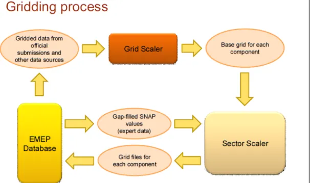
2.2.3.2 The EMEP gridding process

EMEP, under the convention for long range air pollution, has a long experience with the downscaling of reported data in order to run their EMEP model. Depending on the provided data they have different methods, Figure 4 shows the general approach.

(14)

Figure 4: general approach of the EMEP methodology for downscaling of data. 2.2.3.3 Edgar database

JRC maintains a global, gridded database with the most important AQ and GHG emissions (See: http://edgar.jrc.ec.europa.eu/overview.php?v=42). The database is regularly updated on the basis of scientific insights. Edgar can be of help as an independent dataset for those regions where there is a lack of officially reported data; but also as a check for data reported by countries. Furthermore, the fact that Edgar is regularly updated is a big advantage compared to projects where emissions are gridded as a one-off activity.

The availability of Edgar data allows for a modelling exercise at a more detailed level, combining global scenario’s with downscaled calculated emissions that can be applied in atmospheric dispersion modelling. In that sense, Edgar may help in downscaling AP/ GHG metrics to a regional / country level.

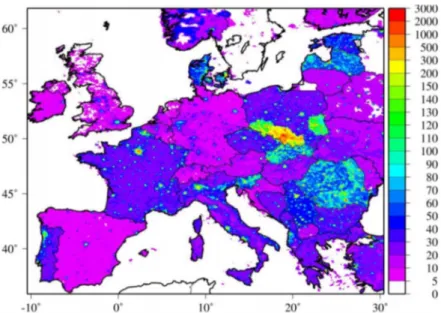
2.2.3.4 TNO/MACC and INERIS/EC4MACS approaches

There are several possibilities to downscale emissions up to a resolution of about 7km from the emission totals provided at country-scale or on coarse geographical grids (e.g. the 50km resolution of EMEP emissions) using external proxies. TNO and INERIS (Figure 5) are both developing such approaches. Both use high-resolution population density maps to re-distribute residential emission and road network maps for the traffic sector. Using the large point source location and fluxes provided in E-PRTR is also standard practice.

(15)

Figure 5: Total annual primary particle emission with diameter below 2.5 µm attributed to the residential sector (g/km2₎ (Terrenoire et al., 2013).

2.2.3.5 IER (Univ. Stuttgart)

In 2010/2011, the University of Stuttgart (Theloke et al) developed a European overview of gridded emissions on the basis of emissions reported by the EU countries under E-PRTR provisions. The results were presented e.g. during the meeting of the Task Force Emission Inventories and Projections (TFEIP) in 2011 (http://tfeip-secretariat.org/2011-tfeip-meeting-sweden/).

As discussed during this task force meeting, the proxies applied in this study for Europe are the same for all countries. That is, on one hand, an advantage, because it increases comparability and consistency in the gridded dataset . On the other hand, specific circumstances per country are not taken into account. For assessing the related uncertainties, Theloke compared his Europe-covering approach with the gridded emissions for the Netherlands; and more specifically NOx from residential combustion. The results of this exercise are shown in Figure 6.

Figure 6: relative differences (in %, NL PRTR compared to IER study) between NOx emissions attributed to Residential combustion according to a national gridding and a European approach due to differences in proxies as applied for gridding the same overall national total emissions for this sector.

(16)

2.3 Summary and ways forward

2.3.1

Air and Climate emission projections

To get more information about the current status of the research in the area of integrating Air Quality and Climate Change and on possible ways forward, an interview was conducted with a number of experts in the field. The results of the interviews are synthesized here:

1. It should be noted that in recent years scenario studies the number of scenarios addressing both fields has increased and both the Air Quality community (TSAP) and the Climate Change community (RCP) have conducted an in-depth scenario for the medium to long-term horizon. 2. Global emission inventories and - in turn - scenarios often have a limited spatial

representation of the EU (a few regions). European assessments requires a spatial resolution of national scale and in some cases down to gridded/agglomerations. Proposed is that EEA

will further develop methods to downscale emission data for instance by following the examples of the developments conducted by TNO (MACC) or INERIS (EC4MACS) in producing high-resolution pan European inventories. There are also ongoing activities in a number of EEA member states (e.g. France, UK, Netherlands, Spain,...) to develop resolutions (~1km) bottom-up inventories. There is scope to make use of such high-resolution inventories as proxies to produce high-quality inventories consistent with officially reported emissions at the country level, as initiated by INERIS for the EuroDelta exercise in support of the CLRTAP/TFMM6_.

3. Most existing projections are focused on regulatory and/or technological alternatives. Air pollution is often focused on EOP, being the economic costs with lowest uncertainty; it is more straightforward than an integrated approach including structural changes and taxation of remaining emission damage on the environment. It is important to include more

structural/behavioural options in scenarios (i.e. reduced meat consumption, efficient use of

heating in houses, taxing damage to the environment, ...) . It is proposed that EEA takes the initiative to explore this approach.

4. Scenarios are often developed with a climate change policy first and then some additional AQ policies are added. It is proposed that EEA would develop a scenario the other way

around, i.e. first define stringent AQ policy till 2050, calculate the co-benefits for CC and derive the remaining policies required to reeds the T-CC target.

2.3.2

Comparing reported emission data

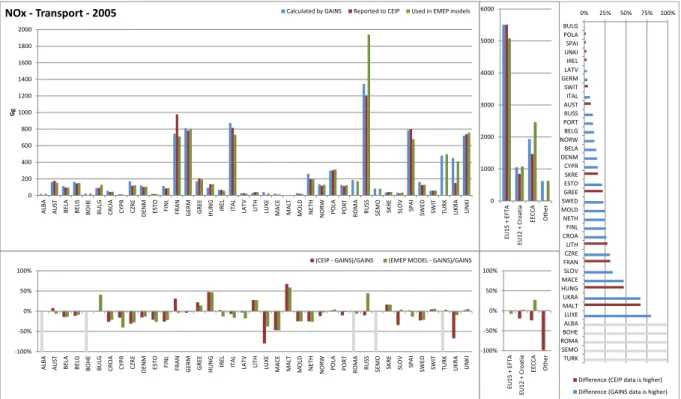
The reported data to the various bodies responsible to collect emission data and used in dispersion models can differ substantially. Therefore scenario studies can differ in outcome, even if they include the same measures. The base year for the calculation and the source used is therefore important. Figure 7 shows national emissions, for the same base-year, for three different, well-known sources. As can be seen easily there are remarkable differences. Climate change and air quality communities use often different datasets for their base year data, it is therefore important to note this and if possible find methodologies to deal with these differences. As a minimum, transparency is needed on base year, which measures are included and how they are taken into account in the scenario analysis. As found by ETC/ACM 2011 (ETC/ACM Technical paper 2011/20 Cobenefits of Climate and Air Pollution Regulations), this is not always reported transparently. In some cases, using relative

changes instead of absolute changes can be a solution instead of emission total for the present day are more robust across inventories.

6_{https://wiki.met.no/emep/emep-experts/tfmmtrendeurodelta}

(17)

Figure 7 Overview of differences in reported emissions for three different purposes (Emissions as reported by countries under LRTAP (CEIP), EMEP model and GAINS approach),

(source: http://www.ceip.at/fileadmin/inhalte/emep/pdf/gridding_process.pdf). 2.3.3

Spatialisation of emissions

Substantial progress has been achieved in improving the spatial distribution of emission inventories, especially over Europe. The topic remains however in development as part of research projects whose limited duration raise a concern of continuity given that such endeavour require periodical updates.

Further development of high-quality proxies for downscaling using a top-down approach is still needed until high-resolution bottom-up inventories such as those available in France and UK and developed in the Netherlands are generalized across the continent. Agriculture is amongst the

activity sectors where such proxies are still highly uncertain. Top-down approaches offer the benefit

of relying on consistent proxies across a wide geographic area. However for the sake of completeness, such proxies are often superficial so that bottom-up inventories are generally

considered higher in quality. In addition these downscaling gridding exercises do not take into

account changes in economic structure over time; so that they are linked to the current (economic) circumstances. Whereas a change in economic structure over time in a country may of course also lead to a change in the distribution of emissions in a country.

0 200 400 600 800 1000 1200 1400 1600 1800 2000 AL BA AU ST BE LA BE LG BO HE BU LG CR O A CY PR CZ RE DE N M ES TO _FINL FR AN G ER M G RE E HUN G IRE L IT AL LA TV LIT H LU XE MA CE MA LT M OL D N ETH N O RW POL A PO RT RO M A RU SS SE M O SK RE SL O V SP AI SW ED SW IT TUR K UK RA UN KI Gg

NOx - Transport - 2005 Calculated by GAINS Reported to CEIP Used in EMEP models

-100% -50% 0% 50% 100% AL BA AU ST BE LA BE LG BO HE BU LG CR O A CY PR CZ RE DE N M ES TO _FINL FR AN G ER M G RE E HUN G IRE L IT AL LA TV LIT H LU XE MA CE MA LT M OL D N ETH N O RW POL A PO RT RO M A RU SS SE M O SK RE SL O V SP AI SW ED SW IT TUR K UK RA UN KI

(CEIP - GAINS)/GAINS (EMEP MODEL - GAINS)/GAINS

0% 25% 50% 75% 100% BULG POLA SPAI UNKI IREL LATV GERM SWIT ITAL AUST RUSS PORT BELG NORW BELA DENM CYPR SKRE ESTO GREE SWED MOLD NETH FINL CROA LITH CZRE FRAN SLOV MACE HUNG UKRA MALT LUXE ALBA BOHE ROMA SEMO TURK

Difference (CEIP data is higher) Difference (GAINS data is higher) 0 1000 2000 3000 4000 5000 6000 EU 15 + EF TA EU1 2 + Cr oa tia EEC CA O th er -100% -50% 0% 50% 100% EU 15 + EF TA EU 12 + Cr oa tia EEC CA O th er

(18)

3 Climate impacts

3.1 Introduction

Emissions of greenhouse gasses and air pollutants lead to changes in atmospheric composition and often subsequently climate forcing and changes, and its impacts and responses (known as the DPSIR chain, = Drivers, Pressures, State, Impacts and Response, Figure 8). The climate forcers and air pollutants should not be considered in isolation as they interact at multiple ways. Studies have, for example, shown that reducing emissions from short-living compounds including some air pollutants could be very effective (=in limiting temperature rise) to “buy time” to deal with CO2 and other long-term gasses (Tol, et al, 2012; Solomon et al, 20132013), something that is important from the perspective of preparing the environment and society (=adaptation). Likewise air pollutants can have an effect on the precipitation patterns by affecting the number and size of clouds (Koren et al, 2014) and reforestation (often seen as a climate change mitigation measure) can be a cost-effective abatement measure for ground-level ozone and nitrogen oxide (Kroeger et al, 2014).

In order to quantify and communicate the contributions to climate change of emissions of different compounds, and of emissions from different regions/countries or sources/sectors, metrics are needed. Some metrics are designed with specific (policy) goals in mind, such as the compliance with air quality standards (e.g., PM2.5 concentrations), others by contrast have been adopted in policy discussions without the original intention for policy use (Schmale et al, 2014). Note that no single metric can accurately compare all consequences of different emissions in the different stages of the DPSIR chain, and all have limitations and uncertainties (Peters et al, 2011). Furthermore, metric values are also strongly dependent on which processes are included in the definition of a metric, and on input parameters and assumptions used. Regarding the latter, uncertainties increase with longer considered time horizon (Reisinger et al., 2010; Joos et al., 2013) and metrics that account for regional variations in sensitivity to emissions or regional variation in response could give a different emphasis to emissions of specific pollutants.

Using different metrics can result in different estimates of required emission reductions in the short and long-term (Brennan and Zaitchik, 2013). One important issue here is that an equal-mass emissions from different regions can vary in their global-mean climate response, an issue that is especially relevant for less homogeneous distributed/short-lived climate-forcing pollutants (SLCPs) such as black carbon and methane. Reducing emissions of SLCPs can provide immediate (local) benefits for health and agriculture and can considerably mitigate climate change (Worldbank, 2013). Note that without mitigation of CO2, reductions in SLCPs can only delay, but not prevent, a substantially greater warming in the longer term (UNEP, 2011). To effectively integrate air pollution and climate change objectives into SLCP reduction strategies, technical metrics need to be used that capture the benefits and trade-offs from both arenas while avoiding inappropriate substitution between SLCP and CO2 mitigation.

(19)

Figure 8: The DPSIR chain from emissions to climate change and impacts showing how metrics can be defined to estimate

responses to emissions (left side) (and for development of multi-component mitigation, right side). The relevance of the various effects increases downwards but at the same time the uncertainty also increases (IPCC, 2013, figure 8.27)

One of the objectives of this chapter is to present an overview of possible metrics that combine climate forcers and air pollutants. Furthermore, we provide some backgrounds behind these metrics (e.g. on spatial resolution) and how these are included in different models and scenarios (both in section 3.2). Finally, based on the comparison of metrics and the assessment of models and scenarios, the chapter also summarizes some recommendations for future research. In this chapter we focus on the interactions in the atmosphere (“state”). Air pollutants and climate forcers also interact when affecting ecosystems and human health (“impacts”).

Note that we focus here on the direct interlinkages between climate forces and air pollutants with respect to emissions of individual gasses and their concentration. As such, we neglect here indirect interlinkages. For example, acidification, nitrogen deposition and ozone may lead to ecosystem degradation, affecting land-cover characteristics, albedo and thus the climate system (e.g. Sitch et al, 2007).

3.2 Synthetic overview of metrics availability

The total contribution of air pollutants and climate forcers can be quantified and communicated in multiple ways/using different metrics. Here we assess these metrics, and provide information on the advantages and disadvantages. We distinguish between metrics that are based on (changes in) atmospheric composition or emissions. A detailed overview on the methodology and analytical formulation of these metrics can be found in (Aamaas et al., 2013). Furthermore, we evaluate how they have been included in existing European and global scenarios.

3.2.1

Concentration metrics

Radiative Forcing (RF) and more recent Effective Radiative Forcing (ERF) are two metrics that are used to quantify the change in the Earth’s energy/radiation balance - as measured at the top of the atmosphere - that occurs as a result of an externally imposed change like changing atmospheric composition (see IPCC, 2013 for details). The atmospheric forcing is, for example, relevant when assessing the likelihood of limiting long-term global temperature increase up to 2K (=the most relevant policy target in climate change, Van Vuuren et al, 2014, Figure 9).

(20)

Figure 9: Probability of achieving temperature targets as a function of greenhouse gas concentration levels (Source Van Vuuren et al, 2014).

RF and ERF are both expressed in watts per square metre (W m–2_{), often used to assess the total} forcing over the industrial era from 1750 to present (/2011), but also applied in multiple scenario analysis to assess the future forcing (e.g. Thomson et al, 2011 and Shindell et al, 2013). The RF and ERF values are compounds specific. Positive values indicate more incoming radiation and as such a warming of the atmosphere, negative values depict a surface cooling.

There is a need to distinguish between direct/instantaneous and indirect forcing when assessing the effect on the global and regional radiation balance (IPCC, 2013). Direct RF and ERF refer to the change of fraction of light being absorbed (warming) by well-mixed greenhouse gases, tropospheric ozone, stratospheric water vapour or scattering (cooling) by stratospheric ozone and aerosols. Indirect RF and ERF refer to aerosols altering cloud properties resulting in the inference of incoming solar radiation with clouds (cooling) or the formation of contrails or contrail induced clouds by aircraft (warming). E.g. Rosenfeld et al (2014) indicated that only little additional aerosols are need to change cloud characteristics and thus climate change. Other indirect effects are deposition of black carbon on ice and snow resulting in less solar radiation being reflected by these surfaces (warming) with as consequence a faster melting of snow and ice masses (EEA, 2012)

The RF concept has been used for many years and assessments – like IPCC assessment reports - for evaluating and comparing the strength of the various compounds in the atmosphere and mechanisms affecting Earth’s radiation balance and thus causing climate change. The total values of well-mixed GHG has increased about 7% between 2005 and 2011 (Table 5). But the relative contributions of these WMGH Gases were relatively stable; changes were due to increasing emissions. This is somewhat different for most aerosols (Table 6). In the IPCC 4th_{Assessment a best} estimate of their RF of –0.5 ± 0.4 W m–2_{was given for the change in the net aerosol–radiation} interaction between 1750 and 2005 (IPCC, 2007). In the more recent assessment this estimate has been lowered down to –0.35 ± 0.5 W m–2_{(IPCC, 2013). It is noteworthy to emphasise that the range} of uncertainty has increased between the fourth and fifth Assessment Reports, and a recent study reported that this uncertainty range was still substantially underestimated (Samset et al., 2014), highlighting the need to (1) be cautious about policy conclusions that can be drawn on the climate impact of aerosols, and (2) support ongoing research on the topic. In quantitative terms we see now a strong cooling effect of sulphate aerosols and an increased strong warming due to black carbon (Table 6, Figure 10).

From the perspective of synergies between air and climate change, Figure 10 can be summarized in three blocks. First, the well-mixed gasses, consisting of the compounds of the Kyoto plus Montreal Protocol (with an overall historic forcing of about 2.8 W/m2_{up to 2011), where the synergy with air}

(21)

pollution is limited. This is more the case for the second and third block. The second block consists of aerosols, which have in general a cooling effect (historically -0.35 W/m2_{), with the exception of black} carbon). The third block is the group of ozone precursors, consisting of CO, VOCs, NOx and CH4. Increased concentrations result in general in more tropospheric ozone and as such –indirectly- in more warming (historically 0.42 W/m2_{). So, when abatement strategies to limit air pollution in} Europe become implemented, the net effect on the climate system depends very much on the type of measure and related compound.

Table 5: Climate forcing for 2011 and 2005 for the Well-mixed GHGes, based on NOASS and AGAGE data (source IPCC, 2013)

Species Radiative forcing

(W.m-2₎ 2011 2005 CO2 1.82 1.66 CH4 0.48 0.47 N2O 0.17 0.16 HFC & SF6 0.03 0.02 Montréal Gasses 0.33 0.33 Total 2.83 2.64

Table 6: Global and annual mean RF (W m–2_{) due to aerosol–radiation interaction between 1750 and 2011 of seven} aerosol components for AR5. Values and uncertainties from SAR, TAR, AR4 and AR5 are provided when available.

Whereas in the RF concept all surface (e.g. albedo) and tropospheric concentrations are assumed to remain constant, the ERF calculations allow most physical variables (except for those concerning the ocean and sea ice) to respond to perturbations like changes in clouds and on snow cover (these changes occur on a time scale much faster than responses of the ocean - even the upper layer - to forcing)7_{. Hence ERF includes both the effects of the forcing agent itself and the rapid adjustments to} that agent (see Shindell et al, 2013 for more details on ERF). ERF is thus seen now as a more applicable metric to quantify the forcing of those components that respond rapidly to changes in the atmosphere and surface characteristics – like aerosols (IPCC 2013, Figure 10). And even for CO2 the ERF could be different from the RF, because CO2 can also affect climate through physical effects on lapse rates and clouds. However, due to contrary effects it is therefore not possible to conclude whether the ERF for CO2 is higher or lower than the RF. Therefore IPCC had defined a ratio ERF/RF to be 1.0 with an uncertainty in the CO2 ERF to be –20% to 20% (IPCC, 2013). Further note that the calculation of ERF requires longer simulations with more complex models than calculation of RF (IPCC, 2013).

7_See_{http://www.ipcc.ch/publications_and_data/ar4/wg1/en/ch2s2-8-5.html}_{for the way how ERF is defined}

(22)

Figure 10: Radiative forcing (RF) of climate change during the industrial era shown by emitted components from 1750 to 2011. The horizontal bars indicate the overall uncertainty, while the vertical bars are for the individual components (vertical bar lengths proportional to the relative uncertainty, with a total length equal to the bar width for a ±50% uncertainty). The coloured box refers to direct or indirect way of how contribute to the forcing. See text for some assessment of the numbers (Source IPCC, 2013).

By nature, well-mixed GHGs such as CO2 are quite homogenous distributed across the world, and forcing per unit emission and emission metrics for these gases thus do not depend on the geographic location of the emission. These gasses have the largest forcing in warm and dry regions (esp. the subtropics), decreasing toward the poles (Taylor et al., 2011). For the short-living climate forcers (SLCFs) the time scale over which their impact on climate is felt is short. Nevertheless their forcing might be relevant, for example to define the need to rapid adaptation (“buying time”). Their concentration spatial pattern and therefore their RF pattern are highly inhomogeneous, and meteorological factors such as temperature, humidity, clouds, and surface albedo largely affect how concentration translates to the forcing.

3.2.2

Emission metrics

Multiple metrics can be defined to quantify, compare, and communicate the relative and absolute contributions to climate change of emissions of different substances, of emissions from regions/countries or of sources/sectors, and as such to show the co-benefits of policies and measures. Note that no single metric can yet compare all consequences (i.e. responses in climate parameters over time) of different emissions. The choice of metrics depends strongly on (i) the particular consequence one wants to evaluate; and (ii) how comprehensive a metric needs to be in terms of indirect effects, feedbacks and economic dimensions (Peters et al, 2011; IPCC, 2013).

The Global Warming Potential (GWP) and Global Temperature Change Potential (GTP) are two frequently used concepts (See Fuglestvedt et al. (2010) and IPCC (2013) for a detailed description).

(23)

GWP integrates the total radiative forcing of a pollutant over a chosen time horizon due to its emission, relative to that of CO2 (without dimension). As such GWP could be seen as an index for the total energy added to the climate system by a pollutant relative to that added by CO2 (IPCC, 2013). When it comes to assessing the warming potential of non-CO2 traces species, the long lifetime of CO2 also plays a role. Since the GWP of any species is normalized by that of CO2, after a few years the signal becomes dominated by the CO2 warming potential. This feature is illustrated in Figure 11 that shows the absolute GWP of methane, black carbon and CO2 in the coming centuries. The AGWP of CO2 is the same in both plots. Because of their shorter lifetimes, the pulse of CH4 and BC vanishes after a few decades (CH4) or years (BC). Therefore their AGWP (defined as an integral forcing up to a given time) becomes constant. On the contrary, the AGWP of CO2 keeps increasing, so that the GWP of CH4 and BC is eventually constrained by the CO2 response alone.

Figure 11: Absolute and Relative global warming potential (AGWP and GWP) of methane (left) and black carbon (right) compared to the AGWP of CO2, (Fuglestvedt et al., 2012).

In order to avoid this ‘artifact’, the Global Temperature Potential (GTP) was designed as an alternative metric. The GTP is defined as the ratio of change in global mean surface temperature (GMST) at a chosen point in time from the substance of interest relative to that from CO2 (as such without dimension). GTP relies on the temperature perturbation (instead of the radiative forcing) at a given time horizon (instead of cumulated up to a given time horizon). By including the climate response in its design, the GTP copes for the shorter lifetime of near term climate forcers by taking into account the longer term impact of the perturbation transferred to the climate compared to the lifetime of the compound itself.

The behaviour of GTP is quite similar as GWP for long lived species. Like GWP, the GTP values can be used for weighting the emissions of greenhouse gasses and pollutants to obtain “CO2 equivalents”. This gives the temperature effects of emissions relative to that of CO2 for a chosen time horizon. For an analogous to GWP that integrates temperature effect up to a given horizon, one can refer to the integrated GTP (iGTP), (Olivié and Peters, 2013).Both for GWP and GTP the choice of the time horizon has a strong effect on the relative importance of near-term climate forcers and well-mixed GHGs to the total forcing. When, for example, using a very short time horizon, short-term climate forcers, such as black carbon, sulphur dioxide or CH4, can have contributions comparable to that of CO2 (of either the same or opposite sign), but their impacts become progressively less for longer time horizons over which emissions of CO2 dominate (IPCC, 2013).

(24)

Figure 12: Global anthropogenic present-day emissions in terms of Global Warming Potential (GWP) and the Global Temperature change Potential (GTP) for selected time horizons. Units are ‘CO2 equivalents’, which reflects equivalence only in the impact parameter of the chosen metric, given as Pg(CO2)eq (left axis) and PgCeq (right axis). Source: IPCC, 2013

In contrary to GWP, GTP is for the moment only used in the physical science framework (Fuglestvedt et al., 2010; Shine et al., 2007), although its advocate make the case for its use in the policy arena to address SLCPs. The fundamental different characteristics of GTP compared to GWP are:

- GWP is a metric that integrates over time, i.e. puts equal weight on all times between the emission and the time horizon. GTP, in contrary, is an “end-point’’ metric, i.e. the temperature change at a particular time in the future (e.g. plus 2o_C).

- GTP takes into account the transfer of energy of the radiative forcers to the climate system. While the GWP of a species is zero once it has exceeded its lifetime (i.e. has been removed from the climate system), the GTP takes into account the fact that the species has transferred energy to the system, and that inertia shall be added to the lifetime of the radiative compound itself. This feature is of course specifically relevant for SLCPs that have, by nature, a shorter lifetime because of their physical (e.g. wet deposition) or chemical (oxidation) removal from the atmosphere.

- GTP is further down the cause and effect chain from emissions to impacts (DPSIR), causing also greater uncertainty (Figure 8). For example, GTP requires additional information such as climate sensitivity.

- Despite that there are significant uncertainties related to both GWP and GTP, the uncertainties of GTP are larger than those of GWP. For the 100-year absolute GWP of CO2 the uncertainty can be as large as ±26%, for CH4 even ±40% (Reisinger et al, 2011; Boucher, 2012). The fact that GTP has been introduced more recently and addressed in relatively less studies than GWP also contribute to this higher uncertainties.

The use of GWP and GTP has advantages and disadvantages. An advantage is that both are suited to address the climate impacts of past or current emissions attributable to various activities. From this perspective, the energy and industry sector has the largest contributions to warming over the next 50 to 100 years, while animal husbandry, waste/landfills and agriculture are relatively large contributors to warming over time horizons up to about 20 years (due to the large emissions of CH4 (IPCC, 2013).

(25)

Limitations deal, for example, with:

• inconsistencies related to the treatment of indirect effects and feedbacks, for instance, if climate–carbon feedbacks are included for the reference gas CO2 but not for the non-CO2 gases;

• The uncertainties related to both GWP and GTP increase with time horizon, complicating the application for assessing long-term strategies (e.g. 20-year absolute GWP of CO2 is about 18%, for 100-year GWP, 26%);

• The choice of metric and time horizon is related to a particular application (implicit value-related judgements) and which aspects of climate change are considered relevant in a given context. At the same time, the values are very dependent on chosen time horizon;

• Metrics do not define policies or goals but facilitate evaluation and implementation of multi-component policies to meet particular goals.

Given these uncertainties and limitations, the type of metric chosen and selected time horizon may have for many components a much larger effect than improved estimates of input parameters (IPCC, 2013). This is important when assessing perceived impacts of emissions and abatement strategies. For example, Wang et al (2013) have shown that when the country's GHG emissions are calculated with GTP instead of GWP, the shares of, for example, the EU and USA rise in the period 1990-2005, and those of some other countries like Australia, China and India decrease. According to these authors, the reason for this may be found in the structure of GHG emissions, particular in the share in which methane emissions contribute to the total emissions of a country. More research would be needed to clarify this.

Another example of the importance of uncertainties in climate metrics is presented in Figure 13. This shows the GWP of TSAP scenarios split by air pollutant when using either default or upper/lower estimates of GWP20. Using default values, it is found that the overall effect of these SLCPs is small, but negative (=cooling) for the period 2010 to 2025. When, however, using the given upper values the overall effect of the air pollutants becomes positive (warming). Especially the wide range in GWP values for BC caused this change. This shows the significance of the uncertainty of these pollutants to the future climate and in particular the uncertainty around black carbon is very large.

Figure 13: Uncertainty of EU28 emissions in the TSAP 2013 scenarios expressed as GWP20 for each compound, and net effect (white dots)

(26)

More recent new metrics have been or are being developed, partly based on the original GWP and GTP concepts (IPCC, 2013) (see Table 7 and Table 8). This to (i) tackle some of the shortcomings of these approaches and (ii) to include more economics dimensions. Examples are:

- GWPbio and GTPbio to assess the effectiveness of biomass combustion for energy, i.e. include the time lag between combustion/use of biomass and regrowth/CO2 uptake of plants. During this period CO2 is resident in the atmosphere and leads to an additional warming (Cherubini et al., 2011);

- Absolute Regional Temperature Potential (ARTP) is an metrics for better capturing the sub-global/regional patterns of responses (Tol et al., 2012; Shindell, 2012; Collins et al., 2013). ARTP gives the time-dependent temperature response in four latitude bands as a function of the regional forcing imposed in all bands;

- Component-by-component or multi-basket approach (e.g. Smith et al., 2012). In this approach multiple gases are divided into two baskets (gases with long lifetimes and short-lived gases, incl. CH4). The two baskets are then presented two metrics that can be used for estimating peak temperature for various emission scenarios.

- Global Cost Potential (GCP) which is the estimated costs for emission reduction that are needed to attain certain climate target (Toll et al, 2012, UNFCCC, 2012; Ekholm et al, 2013); - Climate Change Impact Potential (Kirschbaum et al, 2014). This new is based on explicitly

defining the climate change perturbations that lead to three different kinds of climate change impacts (1) those related directly to temperature increases; (2) those related to the rate of warming; and (3) those related to cumulative warming.

Overall these new metrics have been applied only in few studies. And for the Climate Change Impact Potential, values are only available for the greenhouse gasses (Kirschbaum et al, 2014). As such more research and applications are needed to assess the usefulness and robustness of results (Shindell et al., 2012, IPCC, 2013).

Table 7: GWP and GTP values (without dimension) for greenhouse gasses for a time horizon of 20 and 100 years (based on IPCC, 2013; Joos et al., 2013). Note that numbers do not include climate feedbacks (see IPCC, 2013 for discussion on this). GHG GWP GTP 20 100 20 100 CO2 1 1 1 1 CH4 84 28 67 4.3 N20 264 265 277 234 F gasses HFCs HFC-23 10800 12400 11500 12700 Kyoto HFC-32 2430 677 1360 94 HFC-41 427 116 177 16 HFC-43-10 4310 1650 3720 281 HFC-125 6090 3170 5800 967 HFC-134 3580 1120 2660 160 HFC-134a 3710 1300 3050 201 HFC-143a 6940 4800 6960 2500 HFC-152a 506 138 174 19 HFC-227E 5360 3350 5280 1460 HFC-236F 6940 8060 7400 8380 HFC-245c 2510 716 1570 100 HFC-245fa 2920 858 1970 121 HFC-245c 6680 4620 6690 2410 HFC-365m 2660 804 1890 114 PFCs CF4 4880 6630 5270 8040 C2F6 8210 11100 8880 13500 C3F8 6640 8900 7180 10700 C4F10 6870 9200 7420 1100 c-C4F8 7110 9540 7680 11500 C5F12 6350 8550 6860 10300 C6F14 5890 7910 6370 9490 SF6 SF6 17500 23500 18900 28200

(27)

Table 8: Same as Table 7 for air pollutants, (based on IPCC, 2013, Collins et al, 2013)

Pollutant reference GWP GTP

20 100 20 100

Europe Global Europe Global Europe Global Europe Global NOx Fry et al, 2010; Funglesve -39.4 ± 17.5 19 -15.6±5.8 -11 -48.0±14.9 -87 -2.5±1.3 -2,9

Shindell et al., 2009 -108±35 -31±10

CO Fry et al, 2010; Funglesve 4.9±1.5 6 to 9.3 1.6±0.5 2 to 3.3 3.2±1.2 3.7 to 6.1 0.24±0.11 0.29 to 0.55 Shindell et al., 2009 7.8±2 2.2±0.6

NMVOC Fry et al, 2010; Funglesve 18.0±8.5 14 5.6±2.8 4,5 9.5±6.5 7,5 0.8±0.5 0,66

BC Fuglesvedt et al, 2010 1600 460 470 64

Bond et al, 2013 3200 (270 to 6000) 900 (100 to 1700) 920 (95 to 2400) 130 (5 to 340)

OC Fuglesvedt et al, 2010 -240 -69 -71 -10

Bond et al, 2011 -160 (-6 to -320) -46 (-18 to-92)

SO4 Fuglesvedt et al, 2010 -140 -40 -41 -5,7

CFCs CFC-11 6900 4660 6890 2340 CFC-12 10800 10200 11300 8450 CFC-13 10900 13900 11700 15900 CFC-113 6490 5820 6730 4470 CFC-114 7710 8590 8190 8550 CFC-115 5860 7670 6310 8980 HCFCs HCFC-22 5280 1760 4200 262 HCFC-141b 2550 782 1850 111 HCFC-142b 5020 1980 4390 356 others CCl4 3480 1730 3280 479 CH3Cl 45 12 15 2 CH3CCl3 578 160 317 22 Halon 1211 4590 1750 3950 297 Halon 1301 7800 6290 7990 4170 Halon 2402 3440 1470 3100 304 CH3Br 9 2 3 0

3.3 The use of impact metrics in modelling

As indicated earlier, many modelling activities exist nowadays that consider simultaneously air pollutants and climate forcers, either in terms of emissions and/or concentrations (see also Table 9). Especially the EC-IMAGE and PEGASOS projects included the whole range of species. Both projects used radiative forcing (RF) metric to assess the impacts of these gases on warming in a common unit in the world, including Europe (see also Chuwah et al, 2013). The “EU Limits” project also used the RF metric to sum come the concentrations of different species, in order to assess the available emission space before achieving a global temperature increase of 2°C (Van Vuuren et al, 2014). Because of the long-term target, this study looked, however only at climate forcers and ignored the role of air pollutants. The TSAP study includes the (European) emissions of air pollutants and most climate forcers, and computed the concentration pattern of air pollutants throughout Europe (by using EMEP model). And the ECLIPSE project built upon TSAP projections to refine uncertainties on SLCP metrics, including GTP.

Table 9: overview of the metric use in the projects considered in this study

Project Air pollutants

considered Climate forcers considered Emission metrics Concentration metrics

EC-IMAGE X X RF PEGASOS X X RF LIMITS X RF TSAP X X GWP CIRCLE X RF ECLIPSE X X GTP/GWP