Bank net interest margins in a low interest rate environment

BANK

NET

INTEREST

MARGINS

IN

A

LOW

INTEREST

RATE

ENVIRONMENT

Word count: 22.968

Irem Korkmazer

Student Number: 01505861

Supervisor: Prof. Dr. Rudi Vander Vennet

Co-supervisor: Thomas Present

Master’s Dissertation submitted to obtain the degree of:

Master of Science in Economics

This page is intentionally left blank.

CONFIDENTIALITY AGREEMENT

PERMISSION

I declare that the content of this Master’s Dissertation may be consulted and/or reproduced, provided that the source is referenced.

I

Acknowledgements

This master’s dissertation marks the end of my education at Ghent University and is thus the final hurdle before receiving my degree of Master of Science in Economics: Financial markets and institutions. This journey has been beyond expectations, especially if one considers that my last year was dominated by the COVID-19 pandemic. In essence, the virus has not caused any complications while writing this thesis.

In light of this, a few people deserve some words of gratitude. First of all, I would like to thank Professor Rudi Vander Vennet for letting me discover my interest in banking and finance during his inspiring lectures and giving me the opportunity to work on this interesting topic. Secondly, a heartfelt word of thank is addressed to Thomas Present who guided me throughout this whole process with useful insights and was always available to answer all my questions. He did a splendid job in assisting me.

Of course, the past few years would not be complete without some wonderful fellow students and friends. They always managed to put a smile on my face and keep me motivated, even in the toughest times (early morning lectures, exams and while writing this thesis).

Furthermore, I am also very grateful to my parents and brother for their unconditional support and confidence throughout the years.

Finally, to the reader of this thesis, I hope you enjoy the reading!

Irem Korkmazer Ghent, 2020

II This page is intentionally left blank.

III

Table of contents

TABLE OF CONTENTS III

LIST OF FIGURES V

LIST OF TABLES VI

1 INTRODUCTION 1

2 NET INTEREST MARGIN (NIM) 3

2.1. DEFINING NIM AND ITS COMPONENTS 3

2.2. RELEVANCE OF NIM 5

3 THE TRANSMISSION OF MONETARY POLICY ON BANKS 7

3.1. THE INTEREST RATE CHANNEL 8

3.2. THE CREDIT CHANNEL 8

3.3. THE RISK-TAKING CHANNEL 9

3.4. THE PORTFOLIO REBALANCING CHANNEL 10

3.5. SUB-CONCLUSION 11

4 LITERATURE REVIEW 13

4.1. INTEREST RATES AND BANKS’NIMS 13

4.2. LOW-FOR-LONG 16

4.3. THE ROLE OF BANK-SPECIFIC AND MACROECONOMIC CHARACTERISTICS 18

5 ECONOMETRIC PANEL STUDY 20

5.1. METHODOLOGY 20

5.1.1. POOLED OLS MODEL 22

5.1.2. INDIVIDUAL EFFECTS ESTIMATORS: FIXED VS. RANDOM EFFECTS MODEL 22

5.2. DATA AND SAMPLE 23

5.2.1. DEPENDENT VARIABLES 24

5.2.2. EXPLANATORY VARIABLES 24

5.2.2.1. FINANCIAL MARKET CHARACTERISTICS 24

5.2.2.2. BANK-SPECIFIC CHARACTERISTICS 25

5.2.2.3. MACROECONOMIC CHARACTERISTICS 26

5.2.3. DESCRIPTIVE STATISTICS 28

5.3. EMPIRICAL RESULTS 32

5.3.1. POOLED OLS METHOD 32

IV

5.3.3. HETEROGENEOUS EFFECTS OF MONETARY POLICY 41

5.3.3.1. BANK BUSINESS MODEL 49

6 CONCLUSION 54

7 BIBLIOGRAPHY 56

8 APPENDIX 64

A. LIST OF ALL COUNTRIES AND ALL VARIABLES OF INTEREST 64

B. LOANS AND DEPOSITS VIS-À-VIS HOUSEHOLDS AND NFCS 66

C. CORRELATION MATRIX & SCATTERPLOTS 72

D. THE EVOLUTION OF THE 3 SPREADS OVER TIME 76

E. PROPERTIES POOLED OLS REGRESSIONS 77

F. F-TEST FOR INDIVIDUAL EFFECTS 79

G. EMPIRICAL RESULTS POOLED OLS 80

H. EMPIRICAL RESULTS FE 83

I. MARGINAL EFFECTS LIABILITY SIDE:QE+NIRP 86

V

List of figures

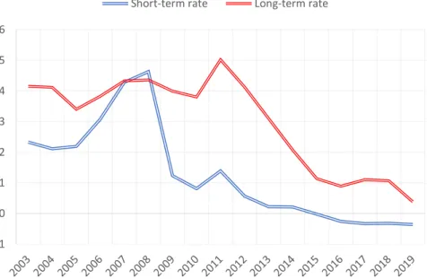
FIGURE 1: COMPONENTS OF NIM ... 4 FIGURE 2: OVERVIEW OF THE TRANSMISSION CHANNELS ... 12 FIGURE 3: EVOLUTION OF THE AVERAGE SHORT- AND LONG-TERM INTEREST RATES ... 30

VI

List of tables

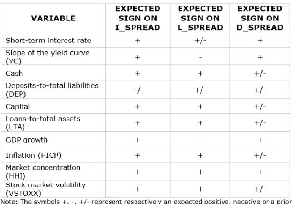
TABLE 1: EXPECTED IMPACT OF EACH VARIABLE ON BANK SPREADS ... 28

TABLE 2: DESCRIPTIVE STATISTICS OF THE (IN)DEPENDENT AND CONTROL VARIABLES ... 30

TABLE 3: EVOLUTION OF THE AVERAGES PER VARIABLE FOR 2003-2019 ... 31

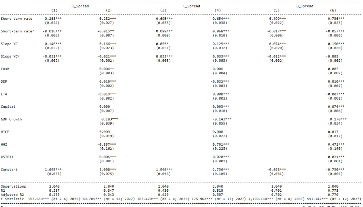
TABLE 4: STATIC MODEL FOR BANK SPREADS ESTIMATED WITH POOLED OLS ... 36

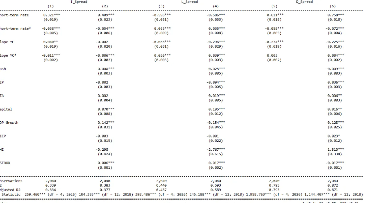
TABLE 5: STATIC MODEL FOR BANK SPREADS ESTIMATED WITH FE ... 40

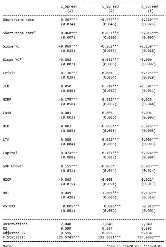
TABLE 6: STATIC MODEL WITH DUMMY VARIABLES ESTIMATED WITH FE ... 44

TABLE 7: STATIC MODEL WITH DUMMIES AND INTERACTION TERMS ESTIMATED WITH FE ... 48

TABLE 8: STATIC MODEL FOR BANK BUSINESS MODEL (DEP) ESTIMATED WITH FE ... 51

1

1

Introduction

Since the Global Financial Crisis (GFC), the economic landscape of many countries has been characterized by low inflation and sluggish growth. Initially, central banks have tried to reverse this situation by pursuing a conventional monetary policy i.e. by lowering their policy interest rates. Even though these key rates have reached their historic lows and bumped into the so-called zero lower bound, the recovery proceeded at a very slow pace (ECB, 2014). Therefore, central banks have decided to adopt a broad range of unconventional monetary policy (UMP) measures such as quantitative easing and forward guidance (Borio & Gambacorta, 2017; Altavilla, Boucinha, & Peydró, 2018). This extra monetary stimulus was intended to further encourage lending, investment and consumption in two ways. On the one hand, they were aimed at lowering long-term interest rates in order to influence the slope of the yield curve. On the other hand, these measures were designed to improve liquidity in the banking system. However, it seems like those monetary policy instruments have failed to fuel the weak economic environment as inflation and growth continue to disappoint. Policymakers are therefore willing to keep interest rates low for as long as necessary (Genay, 2014; Bean, Broda, Ito, & Kroszner, 2015; Nassr, Wehinger, & Yokoi-Arai, 2015; Claessens, Coleman, & Donnelly, 2018).

While monetary policy has a major impact on the interest rate structure, it undoubtedly also influences the banking system (Borio, Gambacorta, & Hofmann, 2017). A traditional bank is mainly engaged in performing maturity transformations, which consists of borrowing short and lending out long (Genay, 2014). This in consequence implies that the net interest income (NII) is considered to be the major source of a bank's total income. However, to judge a bank’s health and efficiency in this role, it is more likely to consider the net interest margin (NIM); calculated as the NII relative to the amount of interest-earning assets (Alessandri & Nelson, 2015; Busch & Memmel, 2015; Angori, Aristei, & Gallo, 2019). Accordingly, it has become of interest to understand how banks’ profitability is affected by volatile interest rates. Especially from the point of view of bank shareholders and other investors, this relationship gained a lot of importance (Claessens et al., 2018; Stockerl, 2019).

2 Against this background, financial experts are convinced that an accommodative monetary policy i.e. a reduction in short-term interest rates and a flattening of the yield curve, have notable effects on the NIM (English, 2002). In particular, a low interest rate environment would significantly contribute to the deterioration of banks’ interest margins (Covas, Rezende, & Vojtech, 2015). Moreover, this negative impact would feed through to banks’ ability to generate adequate profits and eventually harm the soundness of the banking sector (English, 2002; Altavilla et al., 2018).

This short introduction should make clear that it is very important to shed light on the relationship between (low) interest rates and banks’ NIM. It is essential to know how and to what extent a low interest rate environment, caused by an accommodative monetary policy, influences the NIM of banks and which factors (bank-specific and macroeconomic factors) play a role in this. Furthermore, this relationship is also interesting from the perspective of policy makers as it will allow them to evaluate the effectiveness of their monetary policy. Therefore, the overall aim of this thesis is twofold. On the one hand, it gives an overview of how an interest rate environment can affect the banking industry. On the other hand, it quantifies the impact of a changing interest rate environment on banks’ NIM. This master’s dissertation contributes to the existing literature by examining the effect of (low) interest rates on banks’ NIM and its components (deposit spread and loan spread). More precisely, this thesis aims to answer the following questions: “If falling interest rates have left their mark on banks’ NIM, how and to what extent are the separate components of the NIM impacted?” “Furthermore, can we observe any compensation between the loan and deposit spread?”

Using a panel dataset of 2550 banks operating in the 10 countries over the period from 2003 to 2019, we aim to assess the impact of (low) interest rates on the components of banks’ NIM (interest rate spread, lending and deposit spread). By applying static panel models, we find that monetary policy easing (a reduction in short-term interest rates and a flattening of the yield curve) is associated with narrower interest rate and deposit spreads, but wider lending spreads. These results therefore provide strong evidence for the presumption that the components of the NIM on both sides of the balance sheet are asymmetrically affected by changes in interest rates. We further find that a negative interest rate environment weighs on banks’ NIM as it gives rise to an imperfect pass-through of monetary policy measures.

The remainder of this master’s dissertation proceeds as follows: section 2 clarifies the NIM and its components. Section 3 provides an overview of several theoretical mechanisms that outline the interaction between monetary policy and the banking sector. Section 4 then reviews the existing literature concerning the relationship between interest rates and banks’ NIM, whereas section 5 outlines the empirical framework, the data and the results. In the final section, we conclude.

3

2

Net interest margin

(NIM)

Before focusing on the empirical evidence regarding the relationship between the interest rate environment and the NIM, it is important to clearly define the latter. In what follows, we aim to describe this concept and its interpretation based on the existing academic literature.

2.1.

Defining NIM and its components

As already mentioned, the primary business of banks is to channel funds from savers to firms and/or individuals making investments. The net revenues, generated by this activity, are referred to as the NIM. In the literature, some authors simply define the NIM as the difference between the lending rates and the borrowing rates (López-Espinosa, Moreno, & de Gracia, 2011; Busch & Memmel, 2016; Wang, 2017; Angori et al., 2019) while others are more specific in their description and denote it as the difference between interest income and interest expense expressed as a percentage of its average earnings assets (Wong, 1997; Sensarma & Ghosh, 2004; Claeys & Vander Vennet, 2008; Memmel & Schertler, 2013; Genay, 2014; Klein, 2020). This thesis will rather decompose the NIM into several parts after the example of Hempel & Simonson (1999) and examine their development.

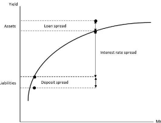
The NIM consists of three components, namely the interest rate spread, the loan spread and the deposit spread (figure 1). First, we’ll consider the interest rate spread. It represents the gap between short-term and long-term interest rates and hence alludes to the slope of the yield curve. In other words, it refers to the earnings of a bank directly obtained by performing maturity transformations. Usually, the yield curve has a positive slope, which implies that long-term rates are higher than short-term rates due to the risks associated with the maturity. Although an upward sloping curve is considered to be normal, it can also be flat or downward sloping depending on changing economic conditions (Hempel &

4 Simonson, 1999). For example, recent economic developments and central bank measures, in particular the asset purchase programmes (APP), have had a significant downward impact on the slope of the curve, making it almost flat. On top of the interest rate spread, financial intermediaries also strive to gain profit on both sides of their balance sheet. On the one hand, banks try to earn a loan spread or commercial loan margin when selecting earning assets. This margin is formed by the wedge between the loan rate and a swap rate with a similar maturity (Busch & Memmel, 2016). On the other hand, if banks are able to attract deposits and raise funds at a lower cost compared to the interbank rate, they will profit from a funding spread or a commercial deposit margin on their liability side (Banking Supervision Committee, 2000).

In addition, it’s worth mentioning that the interest rate spread applies to all banks whereas the loan and deposit spreads are rather bank-specific. This is quite obvious as the former represents the reward on the market while the other two parts demonstrate banks’ efficiency.

5

2.2.

Relevance of NIM

The NIM is often used as a proxy of banks’ profitability. Consequently, one could easily think that the higher the NIM, the more favourable it is. However, this assumption does not hold as there is controversy in the literature regarding the size of the interest margin. Put differently, a high NIM isn’t always a good sign as its interpretation involves a trade-off that will be outlined below.

At first sight, high margins may reflect several positive qualities that banks possess. For instance, high NIMs can be associated with excellent management quality and a high degree of efficiency. This implies that banks with a sound and efficient management are able to choose the most profitable assets and low-cost liabilities in order to boost their interest margins (Maudos & de Guevara, 2004; Angori et al., 2019; Cruz-Garcia, de Guevara, & Maudos, 2019).

Secondly, high margins can also be a sign of a solid capital position, built up by retained earnings. This has three implications. On the one hand, banks absorbing capacity will be increased as they then hold more capital than the minimum capital requirements under Basel III. This in turn will improve the health of the banking sector, thereby contributing to financial stability (Valverde & Fernández, 2007; Shin, 2016; Angori et al., 2019; Klein, 2020). On the other hand, banks can also use the excess capital to expand their portfolio of risky assets. As long as the new assets have an attractive risk-return profile, the interest margins will widen further. Additionally, the level of capital also determines external ratings and investor perceptions as it acts as a signal of banks’ credibility. Better capitalized banks will therefore have the possibility to reduce their funding cost, which will benefit the NIM again (Claeys & Vander Vennet, 2008).

While these aforementioned elements all seem advantageous, we should also look at the other side of the coin since high margins may also reflect some shortcomings. To begin with, several authors (Maudos & de Guevara, 2004; Angori et al., 2019; Cruz-Garcia et al., 2019) state that high margins can only arise in a relatively non-competitive market. After all, in such an environment, banks will have the opportunity to set their prices autonomously thanks to their greater market power. Furthermore, this implicitly means that economic agents will face higher intermediation costs.

Finally, high NIMs can be considered as a reflection of weak supervisory power in a given country. This refers to the capability of official supervisory authorities to directly influence bank behaviour and activity (Angori et al., 2019). So, if the regulatory banking environment is insufficiently developed, this could lead to excessive risk-taking behavior, which will manifest itself in higher margins and ultimately in increased financial vulnerability (Claeys & Vander Vennet, 2008; Angori et al., 2019).

6 Altogether, we conclude that the NIM in itself can give a distorted picture of reality. It is therefore important to interpret this measure taking into account various other factors such as management skills, capital position, competitiveness, supervisory power and many more.

7

3

The transmission of monetary

policy on banks

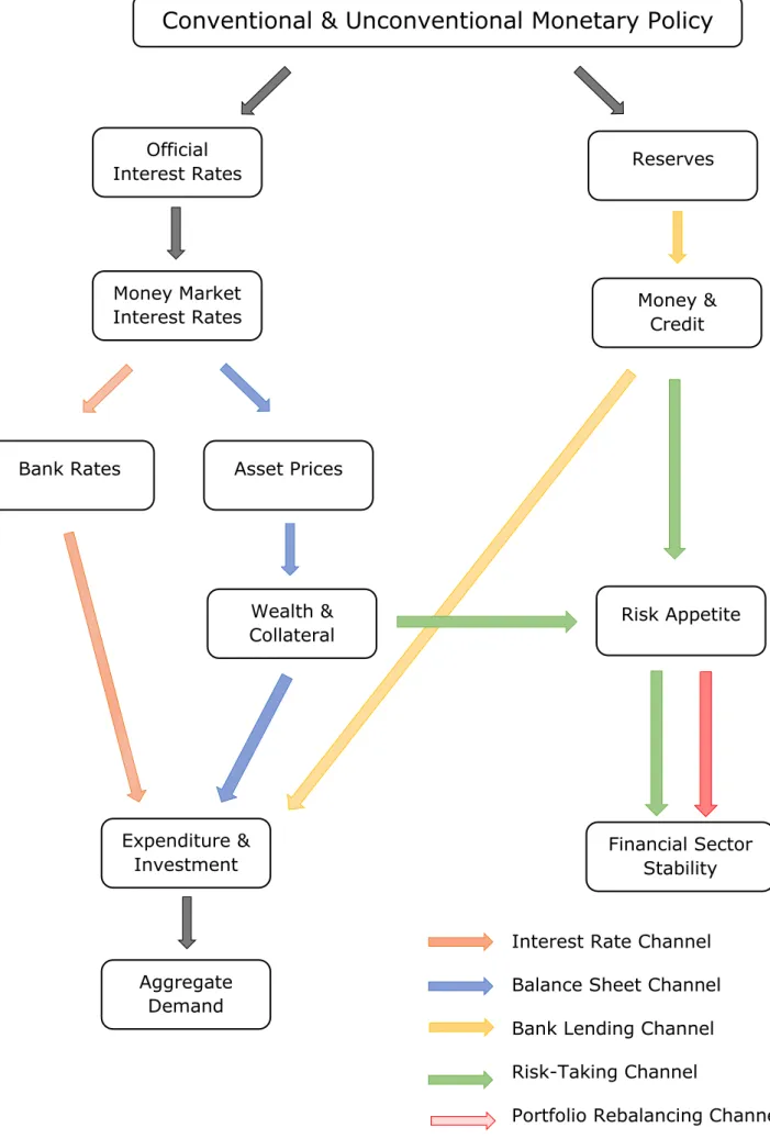
Monetary policy has always been an important factor in determining the behaviour of the banking industry, whether it is conducted conventional or unconventional. Especially in the wake of the financial crisis, the additional non-standard measures have thoroughly changed banks’ liquidity and income structure (Bernoth & Haas, 2018). One of the key moments was the implementation of the negative interest rate policy (NIRP) (ESBG, 2016). Several central banks (Swedish, Danish, European, Swiss and Japanese) decided to loosen their monetary policy even more by pushing the deposit facility rate into the negative territory. As a result, banks had to pay interest to place their excess liquidity with the central bank (Alessandri & Nelson, 2015; Klein, 2020). Mario Draghi, the former president of the ECB, justified this policy by saying that negative rates were the only way to quell market expectations concerning the future course of official interest rates. Otherwise, the private sector would revise its long-term expectations upward, which would significantly affect important economic decisions, thereby undermining the effectiveness of monetary policy (Draghi, 2016; Beyer et al., 2017).

Despite the accommodative stance of monetary policy, the desired results regarding price stability and economic conditions are not forthcoming. Consequently, policymakers are confronted with a lot of criticism from politicians, economists and especially banks. In the following paragraphs, we therefore examine how conventional (reduction in short-term interest rates) and unconventional (flattening of the yield curve caused by quantitative easing & NIRP) monetary policy measures are transmitted to the banking sector. In other words, we distinguish four theoretical transmission mechanisms through which an accommodative monetary policy flows to banks, namely the interest rate channel, the credit channel, the risk-taking channel and the portfolio rebalancing channel (see figure 2).

8

3.1.

The interest rate channel

Within this framework, the interest rate channel is often considered to be the main channel of monetary policy transmission as it affects the most important part of financial intermediaries’ income, namely the NIM (Loayza & Schmidt-Hebbel, 2002). After all, lowering policy rates does not only affect the money-market rates but also the bank lending and deposit rates. Usually, banks always try to preserve their NIM when setting their rates for customers. However, this has become very difficult in a low and even negative interest environment. Two reasons were put forward (Beyer et al., 2017). On the one hand, banks find it very hard to adjust deposit rates in line with the declining market interest rates. They believe that passing on negative rates to their retail depositors would only increase the chance of losing them. These rates are therefore not set below zero in contrast to deposit rates to corporate and institutional clients, which may dip below zero. On the other hand, banks have also become reluctant to lower their lending rates. The transition from higher to lower interest rates changed the banking environment, thereby creating more competition among banks and improving overall efficiency. As a result, lending rates have been trending down, making banks reluctant to cut them even more as it would only further impair the NIM (Jobst & Lin, 2016; Shin, 2016; Bikker & Vervliet; 2017; CGFS, 2018).

These two ways of protecting themselves eventually give rise to a slowdown of the pass-through of a loose monetary policy. In other words, the monetary stimulus will not fully reach the economy as households and firms are only encouraged to invest and consume to a limited extent (Garza-Garcia, 2010; Bernoth & Haas, 2018; CGFS, 2018).

3.2.

The credit channel

The banking industry is a key player in helping policymakers achieve its objectives. In this context, the credit channel comes into play as it sheds light on the impact of monetary policy on both supply and demand of bank credit. Traditionally, a further distinction is made within this channel between two different, albeit related, mechanisms, namely the bank lending channel and the balance sheet channel (Ireland, 2010; Beyer et al., 2017; Bernoth & Haas, 2018).

The bank lending channel or the credit channel in strict sense emphasizes the importance of central banks’ UMP for sustaining loan origination (Beyer et al., 2017). It posits that a policy-induced interest rate drop causes a decline in the opportunity cost of holding deposits. Subsequently, as bank deposits rise, bank reserves will also increase, creating more funds to lend. The increased availability of credit leads then to eased borrowing constraints and triggers banks to expand their loan portfolio. This eventually translates into higher consumption and more investments by households and firms, fostering economic growth (Bernanke &

9 Blinder, 1988; Bernanke & Gertler, 1995; Hernando, 1998; Disyatat, 2010; Apergis, Miller, & Alevizopoulou, 2012; Bean et al., 2015).

However, it should be noted that in a world with three assets - money, bank loans and government bonds - three important conditions must be fulfilled for this channel to work. First, money shouldn’t be neutral, at least in the short run. This means that market imperfections must exist such that prices cannot fully and immediately adjust to money supply changes (Apergis et al., 2012; Peek & Rosengren, 2013). Second, central banks should be able to influence the quantity of loans in the banking system (Oliner & Rudenbusch, 1995; Farinha & Robalo Marques, 2001; Disyatat, 2010; Apergis et al., 2012). Third, bank loans should be an imperfect substitute for other types of finance. This implies that activities of economic agents depend on the availability of credit. In other words, they shouldn’t be able to fully switch to other funding sources such as savings, donations, commercial papers or loans from finance companies for any transaction in the economy (Oliner & Rudenbusch, 1995; Hernando, 1998; Gambacorta, 2005; Apergis et al., 2012).

Unlike the bank lending channel, the balance sheet channel, also known as the broad credit channel, states that monetary policy modifies the balance sheet of borrowers, thereby altering credit demand (Bernanke and Gertler, 1995; Kishan & Opiela, 2000; Bernoth & Haas, 2018). More precisely, a loose monetary policy is expected to improve the health of households and firms in terms of both net income and net worth. Regarding borrowers’ net income, a drop in key interest rates has a dual effect. On the one hand, it reduces borrowers’ interest costs and on the other hand, it boosts firms’ revenues since such a policy is intended to spur the economy. With respect to the net worth, borrowers’ assets are discounted using lower interest rates, increasing the value of their collateral. Combining both factors - increase in wealth and asset prices - strengthen the financial position of households and firms, which in turn induces a decline in the cost of borrowing, more specifically the external finance premium1_{. Their increased borrowing ability} will subsequently be reflected in higher demand for credit, leading to a thriving economy (Bernanke & Gertler, 1995; Kishan & Opiela, 2000; Peek & Rosengren, 2013; Bernoth & Haas, 2018).

3.3.

The risk-taking channel

Banks' perception and tolerance of risk vary over time and are subject to interest rate policies pursued by central banks (Beyer et al., 2017; Dell’Ariccia et al., 2017). Rajan (2005) and Borio & Zhu (2008) were among the first to point this out by suggesting that a low interest rate environment stimulates the risk appetite of banks on both sides of their balance sheet.

1 _{The difference between the cost to the borrower of raising external finance and the opportunity}

10 On the asset side, the increased risk appetite translates into a search-for-yield behavior. Banks are willing to take on more risk, especially when they are faced with a decline in their income from financial assets and therefore unable to meet their nominal return targets (Gambacorta, 2009; Beyer et al., 2017; Bonfim & Soares, 2017; Bernoth & Haas, 2018). Low interest rates also indirectly affect the quality of loan portfolios because it alters banks’ risk perception. At first glance, the banking sector assumes a decrease in credit risk due to the positive impact of low interest rates on asset and collateral values (supra section 3.2.). As a result, they adjust their estimates of default probabilities on outstanding loans downwards and reduce their provisions for non-performing loans. More specifically, banks start to overestimate borrowers’ repayment capacity, which entices them to soften their lending standards and issue more loans. Consequently, these developments amplify the bank lending channel and lead to less qualitative loan portfolios and considerable risk positions (Paligorova & Sierra, 2012; Bikker & Vervliet, 2017; Delis, Hasan, & Mylonidis, 2017; Neuenkirch & Nöckel, 2018).

The risk-taking channel also takes place along the liability side. In particular, banks have the intention to increase their leverage ratio in view of a declining cost of debt ascribable to monetary easing. In other words, they would rather finance themselves more with debt than with equity since it will be more profitable (Adrian & Shin, 2009; Delis et al., 2017; Bonfim & Soares, 2017) However, the extent to which banks can switch to debt financing depends on two elements (Dell’Ariccia et al., 2010; Valencia, 2014). First, banks should be able to adjust their capital structure at the time of a cut in policy rates. In that case, lower rates will lead to lower bank monitoring and greater leverage. Second, debt contracts should afford limited liability protection to banks. This will result in a greater willingness to take on more risk as banks will suffer no losses in case of failure.

3.4.

The portfolio rebalancing channel

As mentioned earlier, the asset purchase programmes (APP) and the introduction of the NIRP have been defining moments in the course of monetary policy. So far, we have shown that these measures had an impact on various aspects of the banking system, such as the interest income, the willingness to lend, the quality of banks loan portfolios and their attitude towards risk. However, we can bring all these elements together under one umbrella as they give rise to the portfolio rebalancing channel (Gambetti & Musso, 2017).

The crucial starting point for this channel is the impact that the APP has on the yield of an asset. That is to say, central banks exert a direct effect on the supply of an asset by purchasing the asset in question. Thus, for a given demand, this results in a decreased availability of that asset in the market which pushes its price up. Due to the inverse relationship between the price and the yield, this process ends in a lower yield for that particular asset. Moreover, this means that the return that banks are hoping to receive in the future will be adjusted downwards. Several

11 authors (Shah, Schmidt-Fischer, & Malki, 2018; Tischer, 2018; Lane, 2019; Bottero, Minoiu, Peydró, Polo, Presbitero, & Settle, 2019) claim that banks don’t throw in the towel because at that moment the portfolio rebalancing channel kicks in. Once the yield differential between the asset classes increases, banks are incentivized to rebalance their portfolios in order to preserve their profitability. In other words, portfolio rebalancing will then not only take place between different maturities, but also between different asset classes. This effect is further enhanced by implementing the NIRP. Negative rates penalize the holding of safer, more liquid assets thus prompting banks to shift to riskier, higher-yielding and less liquid assets. For instance, bank-asset managers are inclined to switch from low-risk government bonds to higher-yielding corporate and emerging market bonds or to corporate loans (Gambacorta, 2009; Beyer et al., 2017).

In addition, Borio et al. (2015), Delis & Kouretas (2011), CFGS (2018) and Brei, Borio, & Gambacorta (2019) discuss another way in which banks can rebalance their portfolio, namely by switching from traditional interest-generating activities to more non-traditional i.e. fee-related and trading activities. In this way, banks reduce their interest rate exposure and maintain their level of income. It is worth noting that this channel could have undesirable consequences in the long term. While it may encounter shrinking margins and profits in the short term, it also increases banks’ risk exposure to financial markets, which in turn could harm the soundness of the banking industry in the long run.

3.5.

Sub-conclusion

The aforementioned transmission channels reveal the inseparability of monetary policy and the banking system. After all, the decisions of policymakers will set the tone for banks behavior and financial stability (Capie, Mills, & Wood, 2018). Theoretically, there is uncertainty about the effectiveness of monetary policy instruments - conventional and/or unconventional - as they produce countervailing effects. On the one hand, a looser monetary policy boosts credit supply, lowers banks’ funding cost and ameliorates the financial position of households and firms. In the latter case, banks also dodge a higher inflow of non-performing loans. On the other hand, historically low interest rates put downward pressure on the NIM and lead to less efficient credit allocation. These elements, in turn, incentivize banks to rebalance their portfolios towards higher-yielding assets, thereby increasing their risk exposure and jeopardizing financial stability. Ultimately, it remains an empirical question whether very low interest rates are beneficial for the banking industry, or for the economy as a whole (Altavilla, Burlon, Giannetti, & Holton, 2019).

12

Conventional & Unconventional Monetary Policy

Official

Interest Rates Reserves

Money Market

Interest Rates Money & _Credit

Bank Rates Asset Prices

Wealth &

Collateral Risk Appetite

Financial Sector Stability Expenditure & Investment Aggregate Demand

Interest Rate Channel Balance Sheet Channel Bank Lending Channel Risk-Taking Channel

Portfolio Rebalancing Channel

13

4

Literature review

Following the interest rate channel, there is a widespread agreement that a low interest rate environment tends to reduce profits, mainly by depressing the banks’ NIM. Surprisingly, however, little empirical evidence on the relationship between interest rates and the NIM has been provided in literature as many studies preferred to use alternative profitability indicators such as the return on assets (ROA), the net operating income margin or the loan loss provisions margin (Genay, 2014; Brei et al., 2019; Klein, 2020). In what follows, we will review the scarce literature in an attempt to clarify the net impact of monetary policy easing on banks’ NIM.

4.1.

Interest rates and banks’ NIMs

English (2002) analyses to what extent changes in market interest rates affect commercial banks’ NIM. The author aims to distinguish short-term effects from long-term effects by using bank data from ten industrial countries over 20 years. In order to conduct this research, English (2002) first formulates two hypotheses. The first hypothesis proposes that interest rate changes reach bank assets and liabilities at a different pace due to the existence of maturity mismatches and repricing frictions. More specifically, returns on liabilities are expected to adjust more quickly to changes in short-term rates compared to returns on assets, which may either amplify or dampen monetary policy shocks (Andreasen, Ferman, & Zabczyk, 2013). So, as long as assets and liabilities are not fully repriced, a decrease in short-term interest rates would temporarily boost banks’ NIM (Heider, Saidi, & Schepens, 2019). The second hypothesis states that a steeper yield curve is presumed to give rise to higher NIMs. This implies that as the yield difference between assets and liabilities increases, banks’ NIM would widen. In line with Borio (1995), Alessandri & Nelson (2015) and Bush & Memmel (2015), regression results provide evidence for the first hypothesis; returns on bank liabilities usually have a shorter repricing period than returns on bank assets. In other words, a reduction in short-term rates will initially increase banks’ NIM. Afterwards, once the repricing process is completed on both sides of the balance sheet, the impact will reverse

14 and hence compress banks’ NIM in the long run. Following these findings, Dell’Ariccia, Marquez, & Laeven (2010) study the knock-on effects that are triggered by this decline. They find that narrow margins are unfavourable for banks’ return on assets (ROA) and ultimately harm their return on equity (ROE). This, in turn, encourages banks to take on more risk and start building up excessive leverage.

Regarding the second hypothesis, English (2002) finds little evidence that the slope of the yield curve has a significant impact on the NIM. While this may seem strange at first sight, it is not inconsistent with most of the literature as they find that the impact of the interest rate spread on the NIM is either very low or statistically insignificant. According to English (2002), this results from the dominant pricing strategy of each bank. For example, if the degree of maturity mismatches between loans and deposits is low, the slope of the yield curve will have little effect on the behavior of the NIM. Similar results and arguments are found by Klein (2020). Interestingly, however, English (2002) also finds no correlation between interest margins and the level of interest rates, which shows that banks in question have successfully limited their exposure to market rates.

A recent study conducted by Hofmann, Illes, Lombardi & Mizen (2020) seems to agree with this last conclusion. They investigate the impact of UMP on retail lending and deposit rates in four euro area countries (Germany, Spain, France & Italy) from 2007 to 2019. Regarding the intermediation margin, they do not find a clear-cut impact of the ECB’s UMP. The results only show a statistically significant decrease in the lending-deposit spread in Germany and Italy. Hence, it turns out that the magnitude of the impact varies widely across countries as it depends on country-specific financial and economic tensions.

In contrast to English (2002) and Hofmann (2020), several other papers (Genay & Podjasek, 2014; Borio et al., 2015; Bikker & Vervliet, 2017; CGFS, 2018; Claessens et al., 2018; Angori et al., 2019; Brei et al., 2019; Cruz-García et al., 2019) with larger datasets draw a different conclusion regarding the latter finding. They re-examine this relationship by relating the NIM to two different monetary policy indicators. On the one hand, they use the 3-month money market rate to represent the short-term interest rate. On the other hand, they take the spread between the 3-month money market rate and the 10-year government bond yield to display the slope of the yield curve. Overall, regression results reveal a positive relationship between the NIM and both monetary policy indicators, confirming conventional wisdom. For example, the study of CGFS (2018) finds that a one percentage point decrease in the short-term interest rate is associated with a 6 basis points decline in the NIM. Furthermore, when allowing for non-linearities by adding quadratic terms of the two explanatory variables to the specifications, the corresponding relationships are found to be concave. The negative coefficients for these terms therefore suggest that the impact of an interest rate change on bank margins are stronger in a low interest environment (Borio et al., 2015; Bikker & Vervliet, 2017; Klein, 2020).

15 Based on the previous findings, Claessens et al. (2018) explore the behaviour of the NIM in different interest rate environments for 3385 banks across 47 countries between 2005 and 2013. To decide whether a country is situated in a low or high interest environment, the authors set a threshold for the three-month interest rate. If the average is less than or equal to 1.25 percent, the country is considered to operate in a low interest environment. Otherwise, if the rate lies above this threshold, it is categorized as a high interest environment. They show that the relationship between the interest margin and an interest rate change is more prominent in a low interest rate environment. More precisely, a one percentage point decrease in the short-term interest rate causes a drop of 20 basis points in banks’ NIM in the low-rate environment, whereas the effect in the high-rate environment is limited to a decline of 8 basis points. Regarding the slope of the yield curve, the results differ in both interest environments. A statistically significant positive association is only found in a low interest rate environment, indicating a higher sensitivity of banks to this variable when interest rates are low. A one percentage change in the slope then leads to a decline of 13 basis points in the NIM. Despite the different methodology, these findings are in line with Borio et al. (2015). Their sample consists of a smaller group of banks in 14 major advanced economies over a period of 17 years (1995-2012). Instead of specifying a threshold, they investigate a one percentage fall in the short-term rate in two possible cases. In the first case, the short-term rate declines from 1 to 0 percent, which reduces the NIM by 50 basis points. In the second case, there is a drop from 7 to 6 percent, pushing banks’ NIM down by just 20 basis points. As for the slope of the yield curve, Borio et al. (2015) prove that the flattening of this curve has a greater impact on the NIM at low interest rate levels than at high interest rate levels.

The previous studies are based on interest rate changes in the positive area. However, as we have already mentioned in this thesis, many economies are now facing negative interest rates. Therefore, it is interesting to explore the difference in impact of both positive and negative rates on interest margins. Using a panel dataset of euro area banks, Boungou (2019) maps the development of the NIM in a negative and positive interest rate environment. Before exploring this field, it is worth mentioning that his findings regarding the relationship between interest rates and banks’ NIM are consistent with the studies above; the short-term interest rate is positively related to the NIM. Moreover, this relationship is characterized by an inverted U-shape. Once this has been established, Boungou (2019) wonders to what extent negative rates have contributed to the deterioration of banks’ NIM. In order to answer this question, he adds an interaction term in his analysis. The results seem to confirm intuition since the coefficient for the negative rates (1.02) is larger than for the positive rates (0.43). In other words, negative interest rates exert a stronger downward pressure on the interest margins compared to positive interest rates. In addition, Klein (2020) reports considerably stronger effects of the positive and negative rates on the NIM, 1.1 percent and 3.2 percent

16 respectively. However, this isn’t surprising as her sample consists of retail banks whose core activity consists of performing maturity transformations.

Altavilla et al. (2018) and Lopez, Rose, & Spiegel (2020) approach this subject from a different angle by scrutinizing the impact of conventional and unconventional monetary policy measures on the main components of bank profitability, being net interest income, non-interest income and provisions. In a certain sense, this study sheds light on the channels above as it focuses on the asymmetric impact of an expansionary monetary policy on banks. Consistent with the findings in other papers, the results display a significant positive relationship between the level of short-term rates and banks’ interest margins. Although this creates a very pessimistic framework for banks in times of unconventional policy, the latter produces countervailing effects. Lowering interest rates appears to have a positive impact on non-interest income and loan loss provisions. Additionally, banks enjoy capital gains due to the increase in the value of the securities they hold. All these positive effects together largely outweigh the negative effect on the margins. Consequently, the authors conclude that under such circumstances banks do not struggle to generate profits. Alternatively, a survey conducted by the ECB (2016) suggests the opposite. More than half of the participating banks declared that the positive effects do not compensate for the loss on their interest margins. Last but not least, the previously mentioned study of Hofmann et al. (2020) also provides evidence for the arguments mentioned in the interest rate channel (supra section 3.1.). Their findings show that the ECB's measures have led to an overall fall in lending and deposit rates. Moreover, the lending rates have been falling more than the deposit rates in all four countries. The authors next identify two significant moments responsible for this deterioration, namely the Outright Monetary Transactions announcement in 2012 and the introduction of the asset purchase programmes since mid-2014. Klein (2020) takes a different view and believes that this effect rather arises from the introduction of the NIRP in the eurozone in June 2014. In contrast to Hofmann et al. (2020) and Klein (2020), Cœuré (2016) argues that conventional and unconventional measures were neither the cause nor the cure for declining rates, as they have been falling since the financial crisis.

4.2.

Low-for-long

So far, much of the empirical evidence reveals that a low interest rate environment has an undesirable impact on banks’ NIM. However, there is disagreement about when this effect will occur, in the short-term or long term. Against this backdrop, policymakers still have a long way to go to bring price stability and the economy to the desired level. As long as these targets are not met, interest rates will be kept low. Consequently, the question arises what impact a prolonged period of low interest rates, also known as low-for-long, will have on banks’ interest margins.

17 Claessens et al. (2018) investigate this question by adding specific variables to their base regression. First, they take into account the number of years that a bank has been in a low interest rate environment. The coefficient for this variable turns out to be statistically significant and negative. In other words, the more time a bank spends in a low interest rate environment, the greater the negative impact on its interest margin. To be more specific, each additional year causes a drop in the NIM of 8 basis points. The authors next wonder whether a time pattern can be found in this effect. Accordingly, they add four dummies representing each additional year in such an environment. The dummy variables for first and second year are found statistically insignificant, indicating that banks’ interest margins are immune to lower rates for the first two years. Regarding the third and fourth year, a low interest rate environment appears to contribute to a decrease of the NIM by 38 and 40 basis points, respectively. These results therefore imply that the effect of low interest rates must be monitored closely as banks ultimately cannot fully protect their NIMs. Similar results are found by the Bundesbank (2015). Based on a sample of 1500 German banks, they show that persistently low interest rates undermine German banks’ profitability, mainly due to shrinking margins.

Along the same line, Demirgüç-Kunt & Huizinga (1999) and Altavilla et al. (2018) find relatively small coefficients for the variables in question. This, in consequence, implies that the downsides associated with UMP will not materialise in the near future. Two reasons are brought forward for this. First, the fact that assets and liabilities are repriced at different times plays in favor of the banks in the short-term (see English, 2002). Secondly, the downward impact on interest margins is counterbalanced by an improved macroeconomic outlook fueled by low rates. After all, favorable economic conditions will initiate the credit channel by stimulating the supply and demand for credit. For example, Brei et al. (2019) detect that the increase in interest margins is mainly caused by a simultaneous increase in the supply of bank demand.

The study of Albertazzi & Gambacorta (2009) sheds light on the relationship between long-term interest rates and the NIM. They establish a negative relationship between a prolonged period of low long-term rates and banks’ NIM. In particular, NIMs will decline by one percent in the first year while after four years this decrease will rise to almost four percent.

Finally, Brei et al. (2019) provide indirect evidence that, in the long term, banks try to offset the deterioration of their interest margins with higher non-interest income, mainly fees and commissions. Results indicate that after one year of low interest rates, the coefficient for non-interest income is only 0.12, whereas after seven years, it rises considerably to 0.37.

18

4.3.

The role of bank-specific and macroeconomic characteristics

We denoted in section 2.2 that various elements contribute to the size of the NIM. So, it goes without saying that some of these determinants will interfere in the relationship between the NIM and the interest rates. That is to say, those elements may either strengthen or weaken the relationship in question, implying that not every bank will be affected in the same way. The literature provides evidence for five factors, namely the size, the business model and the banking and economic environment and inflation.

First, the size of banks plays an important role. For example, Claessens et al. (2018) divide his sample into two groups (small and large banks), based on the size of banks’ assets. He then investigates how the NIM of both groups responds to an interest rate change in a low interest rate environment. The results show that smaller banks are relatively more sensitive to interest rate changes and therefore experience a greater impact on their NIM. The coefficients of a one percentage point decrease in the short-term interest rate for small and large banks are 0.197 basis points and 0.153 basis points, respectively. Genay & Podjasek (2014) also applies the same methodology to banks in the US to shed light on this hypothesis. Although the magnitude of the results differs, small banks’ NIM experience a drop of 1.5 basis points while large banks’ NIM decreases by only 0.3 basis points.

Secondly, the size of the banks is undoubtedly linked to their business model. In general, small banks tend to engage more extensively in maturity transformations and are thus characterized by their typically low level of income diversification. Conversely, large banks are more diversified and carry out other activities such as assisting companies in raising financing capital or providing financial advice during mergers and acquisitions. This results in a more stable income structure and consequently lowers the degree of interest rate exposure (Mergaerts & Vander Vennet, 2015). Following this theory, Memmel (2011) compares savings with private commercial banks and measures the impact of a change in the earnings from term transformation on the interest margin of these two groups. The results for the first group’s NIM (29.2 basis points) are much higher than for the second group’s NIM (6.9 basis points), implying that small banks have greater difficulty to shield their NIMs from low interest rates and hence take the greatest hit. After all, larger banks have the advantage of hedging their exposure to interest rate risk in various ways such as increasing their operational efficiency, switching to trading and fee-based revenues, reducing maturity mismatches by selecting assets and liabilities or attracting other funding sources than deposits. We can therefore conclude that a viable business model in times of low interest rates is characterized by income diversification (CGFS, 2018; Klein, 2020).

Thirdly, the intensity of the relationship between interest rates and NIMs also depend on the nature of the banking market. We distinguish banking markets with

19 low and high concentration. The results illustrate that banks operating in the former environment are more prone to changes in interest rates than banks in the latter environment. Two elements are responsible for this larger impact. On the one hand, banks in a low-concentration market have little power to set their prices (Naceur, 2003). As a result, they are obliged to pass on interest rate drops to their loan customers. On the other hand, a low-concentration market is also characterized by strong competitive pressure, which leaves banks with less latitude to adjust deposit rates (CGFS, 2018).

Fourthly, it might be interesting to consider the economic environment in which banks operate as this largely determines the supply and demand of banking services in the economy (Gros, 2016). Using GDP growth as a proxy, one expects to notice substantial effects on the NIM. However, opinions about the direction of the impact are divided. Altavilla et al. (2018) find that a low economic growth only strengthens the relationship between the NIM and the interest rates. In other words, a low GDP growth creates additional pressure on the NIM in a low interest rate environment. Conversely, Claessens et al. (2018) and Bikker & Vervliet (2017) argue that low economic growth damages debt servicing capacity of borrowers. As a result, banks will charge a higher risk premium which, in turn, will lead to an upward pressure on the banks’ interest margins.

Last but not least, several studies claim that there is a relationship between inflation and banks’ interest margin. But as for the sign of this relationship, there is a disagreement among the authors. Perry (1992) argues that inflation has a differential impact on the NIM depending on whether it is anticipated or not. If inflation is anticipated and borrowers’ real incomes are sticky, we observe a positive association between inflation and banks’ NIM. A rise in inflation will then lead to a deterioration in borrowers’ net worth and creditworthiness, thereby increasing the risk of default. In response to this, banks will charge higher lending rates which will in turn widen the margin (Tarus, Chekol, & Mutwol, 2012). This theory is consistent with empirical evidence provided by Claessens, Demirgüç-Kunt & Huizinga (2001), Honohan (2003), Gelos (2009) and Angori et al. (2019). However, if inflation is not anticipated, the inflation shock cannot be passed through to borrowing and lending rates equally rapidly. In other words, bank costs may increase faster than bank revenues, thereby impairing banks’ NIM (Naceur and Kandil, 2009; Tarus et al., 2012).

20

5

Econometric panel study

The previous section provided a broad overview of the studies conducted with regard to the relationship between interest rates and banks’ NIM. The mixed results regarding the direction of the impact raise the following questions: If UMP of central banks has left its mark on banks’ NIM, does this mean that the components of the NIM - the interest rate spread, the loan spread and the deposit spread - are equally affected? Or is there some kind of compensation going on between loan and deposit spreads to limit the damage?

We aim to answer the above-mentioned questions by performing a cross-country panel data analysis. In the following subsections, the methodology will first be explained in detail. Then the data will be discussed in order to proceed to the results of this research.

5.1.

Methodology

This section presents the estimation strategy employed to scrutinize the link between interest rates and banks’ NIM. Therefore, we first compile a panel dataset that contains repeated observations over the same units (in our case: countries) collected over several periods (Verbeek, 2007; Gujarati & Porter, 2009). Usually, a distinction is made in the literature between micro and macro panels, depending on the number of units and periods. A micro panel, for instance, is characterized by data where the number of units is much larger than the number of periods (n >> T). However, if the situation reverses and the number of units is smaller than the number of periods (n << T), then we speak of a macro panel. Obviously, the former includes more information on a unit-level, making it more suitable to investigate unit heterogeneity. The latter, on the other hand, rather focuses on the time dimension of the data, capturing the dynamics of adjustment (Baltagi, 2008). Altogether, we construct a balanced2 _{macro panel of 10 countries with}

2 _{Balanced panels are defined as complete panels without randomly missing observations (Baltagi,}

21 observations collected over 204 time periods. In this way, we gain insight into the extent to which banks’ NIM adjust to monetary policy changes.

Furthermore, several other advantages are linked to the use of panel data, also known as longitudinal data. For example, it provides a more informative dataset as the sample size is significantly larger compared to cross-sectional or time-series data. As a result, there will be more variability and less collinearity among variables, but more importantly it will yield more efficient and accurate estimates. Especially the combination of cross-sectional and time series data will allow us to specify richer econometric models to identify and measure effects that are otherwise simply undetectable (Kennedy, 2008; Verbeek, 2007).

Finally, a panel study also makes it possible to control for individual heterogeneity, thereby implicitly acknowledging the fact that all units are different from each other. This further entails that the behaviour of each unit is affected by multiple unmeasured, state- and time-invariant explanatory variables, which in turn could alter the relationship in question. A pure cross-sectional or time series analysis, by contrast, does not account for these variables, causing serious misspecifications and leading to biased results. Consequently, panel data considerably reduce the omitted variable problem and allow us to consider country-specific characteristics that influence the impact of monetary policy on banks’ NIM (Hsiao, 2005; Baltagi, 2008).

Although there are a lot of benefits associated with the use of panel data, it does not solve all problems faced by a cross-sectional or time series study. The disadvantages are more of a practical nature such as design and data collection problems, distortions of measurement errors, selectivity problems and cross-section dependence. Despite these limitations, Baltagi (2008) and Verbeek (2007) still argue that it’s worth using panel data as the benefits outweigh the disadvantages.

A general panel data model can be written as follows:

y

it

= α

it

+ x

it′

β

it

+ ε

it

with i = 1, … , n and t = 1, … , T [1]

where the double subscripts (i and t) are indices for units and time, x_it

represents

a K-dimensional vector of explanatory variables for unit i in period t, β_it quantifies the partial effect of x_it on y_it for unit i in period t and ε_it captures the unobservable factors that influences y_it. This model is undoubtedly too general to estimate and to provide useful results. As a result, we’ll have to put some structure on the coefficients, α_it and β_it

, by imposing several assumptions on them. In what follows,

we will distinguish two estimation techniques, namely the pooled ordinary least square (OLS) model and the individual effects model.

22

5.1.1.

Pooled OLS model

The pooled OLS model is considered to be the most stringent of all panel estimation models as it restricts the coefficients (α and β) to be constant across time and units. Moreover, it imposes two strong assumptions regarding the explanatory variables and error terms. On the one hand, all explanatory variables are assumed to be independent of all error terms. On the other hand, error terms are treated as identically and independently distributed disturbances. Consequently, specification [1] turns into

y

it

= α + x

it′

β + ε

it

with ε

it

~ iid(0, σ

ε2

) [2]

The pooled estimator is characterized by a number of properties. First, it exploits both the within and between dimensions of the data. Second, the estimator is consistent for n → ∞ or T → ∞ as long as the explanatory variables are weakly exogenous and uncorrelated with the individual effects. However, we cannot conclude that this model provides efficient estimators as it simply stacks the data and ignores the panel structure. Moreover, due to the nature of our data, the above-mentioned assumptions will no longer be satisfied (see infra section 5.3.1). For instance, we can no longer presume that errors terms from different periods are uncorrelated. Or, it is no longer appropriate to suppose that different observations of the same units are independent from each other. Hence, this approach does not allow for individual country heterogeneity and time effects. Therefore, the pooled OLS method is likely to yield inefficient estimators relative to the other methods and is thus often considered to be impractical.

5.1.2.

Individual effects estimators: fixed vs. random effects model

The individual effects estimators are more appropriate models as they do take the panel structure of the data into account by letting the intercept (α) vary across units. The slope coefficients (β), by contrast, are still considered to be constant for all i and t. Within this category, we speak of fixed effects (FE) or random effects (RE) models depending on the assumptions about the error term. Before going deeper into these models, it is important to mention that both have the ability to control for unobserved country-specific and time-specific effects. In other words, these models pay attention to the unobserved heterogeneity that may not be captured by the explanatory variables included in the model. Subsequently, the omitted variable bias will be significantly reduced, yielding consistent and unbiased estimators (Leyaro, 2015).

The fixed effects model regards unobserved differences between units as a set of fixed parameters and changes equation [1] into

y

_it

= α

_i

+ x

_it′

β + ε

_it

with ε

_it

~ iid(0, σ

_ε2

_{) [3]}

where the individual-specific intercept (α_i) represents those (un)observable time-invariant differences across units. Characteristic for this model is that it does not

23 impose any restrictions upon the relationship between

α

_i and the explanatory variables, thereby allowing for any correlations between them. As for the relationship between α_i

and the error terms, statistical independence is assumed

(Baltagi, 2008; Verbeek, 2008).

Nevertheless, the fixed effects model has some disadvantages. First, this approach will not produce estimates for the variables that do not change over time. Second, fixed effects estimators exploit the within dimension of the data, causing them to ignore any information about differences between individuals. So, if the explanatory variables vary widely across units, but fluctuate only slightly over time for each unit, the estimators will be rather imprecise. This will be reflected in larger standard errors, higher p-values and wider confidence intervals (Allison, 2005; Nwakuya & Ijomah, 2017).

In contrast to the fixed effects model, the random effects model assumes the individual-specific effect to be a random variable that is uncorrelated with the explanatory variables. The model can therefore be written as

y

it

= μ + x

it′

β + ϵ

it

[4]

ϵ

_it

= α

_i

+ ε

_it

with ε

_it

~ iid(0, σ

_ε2

_{) and α}

i

~ iid(0, σ

α2

) [5]

The main difference is that the error term (α_i

+ ε

it) now consists of two

components. On the one hand, it contains the individual specific component (α_i), which is time invariant and homoscedastic across units. The inclusion of this element in the error term explains the assumption above; any correlation between the two variables, α_i en x_it, would lead to biased and inconsistent estimators. On the other hand, the error term also includes an erratic component (ε_it) that is uncorrelated over time and homoscedastic. Unlike the fixed effects model, the random effects model use information both within and between individuals, resulting in more efficient estimates.

5.2.

Data and sample

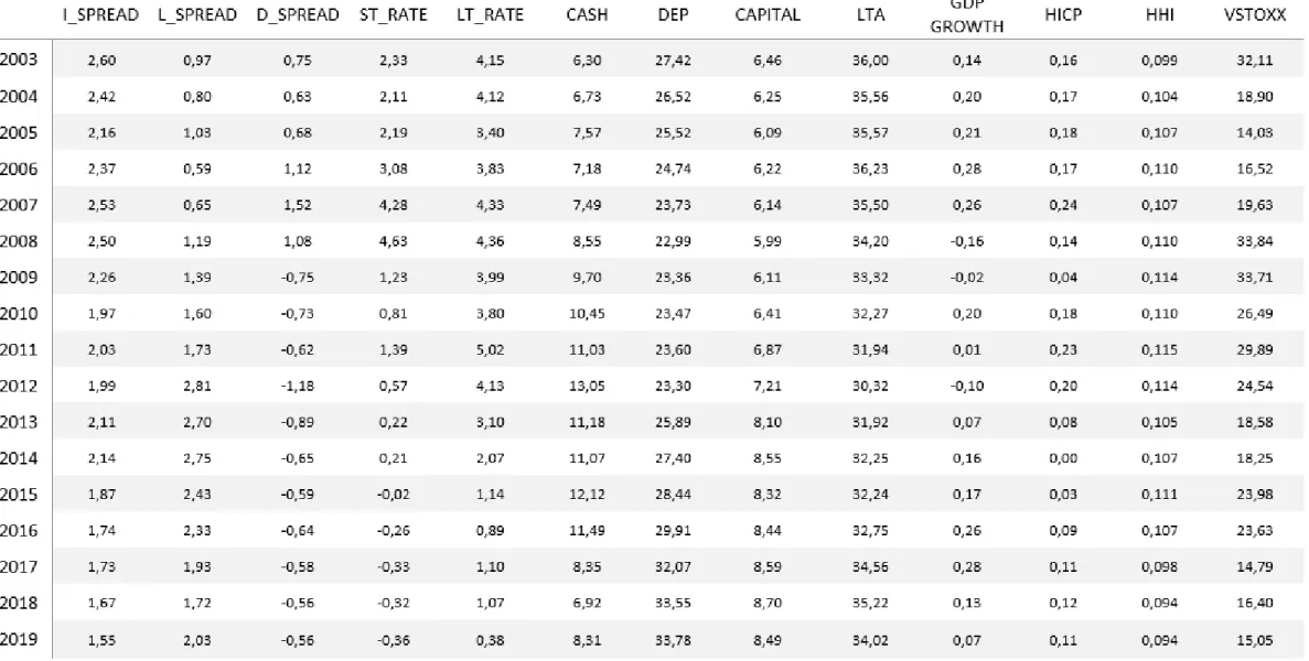
The data used in this dissertation is obtained from Eurostat, Thomson Reuters Datastream and Statistical Data Warehouse (SDW), a database maintained by the ECB. Our sample consist of 2550 bank observations and covers 17 years from 2003 to 2019. Within this time interval, we consider both the years before and after the Global Financial Crisis, which allows us to fully capture the evolution of a low interest rate environment. The 10 countries in study include: Austria, Belgium, Germany, Spain, Finland, France, Ireland, Italy, The Netherlands and Portugal. These countries represent core (6) and periphery countries (4) and are considered due to data availability. In addition, we refer to the appendix A for a list of all countries and a table describing all the variables included in the empirical analyses of this paper.

24

5.2.1.

Dependent variables

As mentioned in section 2, the objective of our study is to determine whether the components of banks NIM are affected by the changes in the interest rate structure. Therefore, we’ll consider three dependent variables.

Our first and main dependent variable is the interest rate spread, which is obtained by taking the difference between lending rates charged by banks on loans to households and deposit rates offered by banks to households. We focus specifically on households because they are the counterparty to most bank loans and deposits in the countries under consideration, except for Austria and Italy (Appendix B). Although the volume of loans to NFCs is roughly the same as that of households, we cannot include this group in our study due to a lack of bank balance sheet data on the liabilities side.

In addition to the main component of the NIM, we are also interested in the evolution of the commercial margins. By taking these into account, we gain insight into how banks’ credit and deposit policy adapts to a changing interest environment.

• On the asset side, we define the loan spread as the wedge between lending rates and the 5-year Credit Default Swap (CDS) rate. The price of a CDS provides a direct measure of the compensation required by the market for insuring credit risk (Norden, & Wagner, 2008).

• The deposit spread on the liability side is computed by subtracting the deposit rates from the 3-month Euro OverNight Index Average (EONIA).

5.2.2.

Explanatory variables

Considering the existing literature on the association between interest rates and banks’ interest margins, we decided to use the following set of explanatory variables. In addition to the description of the variables, we also provide a hypothesis for each variable regarding its expected impact on the NIM and its components.

5.2.2.1. Financial market characteristics

So far, we know that the banks’ traditional business is particularly influenced by monetary policy measures. This implicitly means that money market interest rates are the most critical drivers of banks’ NIM (Angori et al., 2019). In accordance with the above-mentioned studies, we therefore introduce two monetary policy indicators that will reflect the financial market, in particular the interest rate environment.

On the one hand, we use the 3-month EURIBOR rate to proxy the short-term interest rate. The EURIBOR indicates the average interest rate at which Eurozone

25 banks offer to grant loans to each other. The relevant data has been retrieved from Eurostat and contains monthly based information. Following the evidence from various studies, we expect a positive sign for this variable. In other words, an increase (a decrease) in short-term interest rate is expected to move banks’ NIMs upwards (downwards).

On the other hand, the long-term interest rate is represented by the yields of government bonds with maturities of close to 10 years. This variable is, in turn, used to determine the slope of the yield curve, which is approximated by the difference between the long‐ and short‐term interest rates. Once again, monthly data are collected over the period 2003-2019 from SDW. We assume that this variable will have a positive sign as an increase in the slope of the yield curve implies a bigger difference between the interest rate on loans and that on deposits (Cruz-Garcia et al., 2019).

5.2.2.2. Bank-specific characteristics

Assuming that each bank is affected in a different way by monetary policy shocks, we include a set of bank-specific indicators, namely cash, capital and the loans-to-total-assets-ratio and the deposit-to-total-liabilities-ratio. Our first two variables shed light on banks’ liquidity and capital dimension as the financial crisis has shown that insufficient buffers had been built up in these areas. The two other variables refer to the structure of the balance sheet, which will give us some insight into the banks’ business model. Although there are many other bank-related variables, we’ll limit ourselves to these four variables to maintain an overview in this dissertation.

To begin with, cash is considered the most important liquid and safest asset for two reasons. On the one hand, banks need cash to fund their day-to-day operations and to fulfill short-term payment obligations (Borio et al., 2015). On the other hand, cash creates a buffer in times of financial emergencies as it can be used immediately to pay for the essentials and stay on top of the bills (Angbazo, 1997). However, holding excess cash is not the best strategy to follow since it involves an opportunity cost. By maintaining high levels of cash, banks may miss the opportunity to invest in potentially high-yielding assets. To make up for this situation, they tend to pass this cost on to their customers by increasing their interest rates (Garza-Garcia, 2010; López-Espinosa et al., 2011; Angori et al., 2019; Cruz-Garcia et al., 2019). In this vein, a higher amount of cash is associated with higher NIMs. We approximate this variable in the analyses by the ratio of cash to total assets.

A second bank-specific factor is bank capital (CAP) that serves as a buffer against unexpected losses (Yeh, Twaddle, & Frith, 2005). A solid capital cushion does duty as a safety net in difficult times, making it a proxy of bank solvency (Athanasoglou, Brissimis, & Delis, 2008). Alternatively, bank capital also sheds light on banks’