A comparative study of machine learning techniques to predict speed through water and speed loss due to fouling of seagoing vessels

(1)

A COMPARATIVE STUDY OF MACHINE

LEARNING TECHNIQUES TO PREDICT

THE SPEED THROUGH WATER AND

SPEED LOSS DUE TO FOULING OF

SEAGOING VESSELS

Word count: 31.592

Casimir Morobé

Student number: 01508208

Supervisor: Prof. Dr. Dirk Van den Poel

Master’s Dissertation submitted to obtain the degree of:

Master in Business Engineering: Data Analytics

(2)

The content of this master’s dissertation may be consulted and/or reproduced, provided that the source is referenced.

Casimir Morob´e

(3)

(4)

Abstract

In the shipping industry fuel costs can make up to 75% of operational costs. This in combination with environmental considerations makes fuel efficiency a top priority for the shipping industry and its regulators. The main reason for subpar fuel efficiency is the accumulation of marine organisms on the hull and propeller of the ship, referred to as marine fouling. Fouling can lead to an 80% increase in drag resistance and up to 40% increase in fuel consumption. To counter this, vessel operators periodically remove this fouling using hull cleaning, propeller cleaning or dry-docking. Considering the high environmental and financial costs of either continuing operations with decreased fuel efficiency or too frequently performing maintenance operations, it is crucial to have a Decision Support System (DSS) in place to determine when to perform what kind of maintenance. Creating such a maintenance DSS requires the ability to accurately measure the impact of fouling on fuel efficiency. Currently, most vessel operators are not aware of the true impact of fouling on vessel performance, even though the IMO has mandated the monitoring of such factors in the Ship Energy Efficiency Management Plan (SEEMP). Lots of research has been done in this area, indicating that fouling is too complex to be accurately modeled using theoretical, physical models and requires data-driven methods such as Machine Learning. This research compares the effectiveness of multiple ML techniques to solve this specific problem using historical sensor data from a 2550 TEU container ship. In a first step of the Digital Twin approach the speed through water of the vessel is predicted and in a second step these results are leveraged to find the speed loss due to fouling. A comparison of numerous Frequentist and Bayesian ML techniques is made and concludes that although Feedforward Deep Neural Networks provide slightly better results, the Bayesian approach of Gaussian Process Regression (GPR) is preferred

(5)

since next to high accuracy, it is also able to provide confidence intervals for its predictions. Uncertainty estimation is crucial for a maintenance DSS. Finally, an optimization method is proposed to minimize fouling-related costs over time. The research concludes with an economic interpretation of the model and states that if accurate fouling estimation were available during the period before dry-docking, different maintenance decisions would have been taken, leading to a 6.2% decrease in total fuel consumption. After taking maintenance costs into account, this results in a net cost reduction of 2.1%. In conclusion, a data-driven maintenance decision system supported by accurate fouling estimation is presented. It is concluded that such a system enables vessel operators to make fact-based maintenance decisions resulting in considerable economic and environmental value.

Keywords

Machine Learning, Fouling Detection, Ship performance monitoring, Bayesian Machine Learning, Gaussian Processes, Predictive Maintenance, Maintenance Decision Support System

(6)

Preface

This thesis represents the final milestone of my studies Business Engineering at Ghent University. Covering topics such as physics, data science and cost-optimization this research built further on the broad range of knowledge acquired over the past 5 years. This thesis would not have been possible without the data and expertise extended to me by the partnering shipping company. Due to data privacy concerns, I am unable to thank them by name, but I would like them to know that I am extremely grateful for their time and support.

(7)

(8)

List of Abbreviations

ANN Artificial Neural Network BBM Black Box Model

CDP Controlled Depletion Polymers CFD Computational Fluid Dynamics CV Cross-Validation

DFFNN Deep Feedforward Neural Network DNN Deep Neural Network

DS Decision Stump

DSS Decision Support System DT Decision Tree

EDA Exploratory Data Analysis EE Engine Efficiency

EP Engine Power

FOC Fuel Oil Consumption FRC Foul Release Coatings GBM Grey Box Model GP Gaussian Process

GPR Gaussian Process Regression

IMO International Maritime Organization

ISO International Organization for Standardization KNN K-Nearest Neighbor

KRR Kernel Ridge Regression LR Linear Regression MAE Mean Absolute Error

(13)

Contents

MBE Mean Bias Error

MAPE Mean Absolute Percentage Error ML Machine Learning

MLP Multi-Layer Perceptron MSE Mean Squared Error NN Neural Network

OLS Ordinary Least Squares RBF Radial Basis Function RF Random Forest SE Squared Exponential

SEEMP Ship Energy Efficiency Management Plan SP Shaft Power

SPC Self-Polishing Copolymer SRPM Shaft Rotations Per Minute STW Speed Through Water SVR Support Vector Regression TBT Tributyl-Tin

TEU Twenty-Foot Equivalent unit WBM White Box Model

(14)

List of Figures

2.1 Ship Powertrain (Pedersen, 2014) . . . 7

2.2 Worldwide salinity map (Kostis, 2009) . . . 12

2.3 Draft and Trim of a ship (Biran & Pulido, 2013) . . . 13

2.4 Visualization of the complexity of the interaction effects between propeller and rudder (Mofidi & Carrica, 2014) . . . 14

2.5 A ship in fouled condition (Mfame, 2016) . . . 15

2.6 Effects of fouling removal (Munk et al., 2009) . . . 19

3.1 Overview of different modeling techniques (Haranen et al., 2016) . . . 24

3.2 Accuracy of different modeling techniques (Haranen et al., 2016) -WBM (dash-dot), GBM (solid), BBM (dot) . . . 25

4.1 Draft and Trim of a ship (James et al., 2013) . . . 34

4.2 Draft and Trim of a ship (Gillis, 2017) . . . 35

4.3 Visualization of OLS by Lee (2019) . . . 37

4.4 Visualization of SVR . . . 40

4.5 Influence of Kernel on SVR (sklearn, 2007b) . . . 41

4.6 SVR compared to KRR (sklearn, 2007a) . . . 43

4.7 Example of a decision tree (J. Friedman et al., 2001) . . . 44

4.8 Visualization of a random forest (Dambre & Dhaene, 2019) . . . 46

4.9 The AdaBoost algorithm (Freund & Schapire, 1996) . . . 47

4.10 Gradient Boosting algorithm (J. Friedman et al., 2001) . . . 48

4.11 A perceptron (Nielsen, 2015) . . . 51

(15)

List of Figures

4.13 Difference between parameter space and distribution space (Duan et

al., 2019b) . . . 58

4.14 The natural gradient (Duan et al., 2019b) . . . 58

4.15 NGBoost algorithm (Duan et al., 2019a) . . . 59

5.1 Primary features . . . 68

5.2 Secondary features . . . 69

5.3 Correlation Matrix . . . 70

5.4 5-fold Cross-Validation (sklearn, 2020b) . . . 73

5.5 Feature Importance Random Forest . . . 76

5.6 First 5 rows of pre-processed data . . . 76

6.1 KRR Traing Curve . . . 81

6.2 Keras Neural Network . . . 85

6.3 Keras Training Curve . . . 86

6.4 GPR Training Curve . . . 88

6.5 GPR Validation Curve for lengthscale . . . 88

6.6 GPR Predictions with 95% confidence intervals . . . 89

6.7 NGBoost predictions with 95% confidence intervals . . . 90

7.1 MBE error over time intervals . . . 97

7.2 Fouling detection using speed loss . . . 98

7.3 Fouling detection using speed loss . . . 99

7.4 Speed loss for the complete period . . . 100

8.1 Maintenance Decision Support System (Vanden Hautte, 2020) . . . . 105

9.1 The effect of dry-docking on the STW . . . 111

(16)

List of Tables

2.1 Effect of water depth (Patel & Premchand, 2015) . . . 10

5.1 Available data . . . 63

5.2 Standard Features used for modeling . . . 75

6.1 Performance of the different ML models, sorted by MAE . . . 92

9.1 Performance of the different ML models, sorted by MAE (repeated from 6.1) . . . 110

(17)

Chapter 1

Introduction

1.1 Research context

With over 80% of the world trade volume being moved through shipping (on Trade & Development, 2017), maritime transport forms the backbone of the global economy. For the period 2007-2012 shipping emissions represented 3.1% of annual global CO2 emissions and these shipping emissions are expected to rise between 50% and 250% by 2050 (Smith et al., 2015). Even though shipping emissions were relatively overlooked during the 1997 Kyoto Protocol (Loeff et al., 2018), in recent years regulating bodies like the IMO have introduced mandatory measures in an attempt to reduce shipping emissions (Joung et al., 2020). Furthermore, fuel costs can make up to 50%-75% of the total operating costs of large vessels (Rehmatulla & Smith, 2015; Ronen, 2011; X. Wang & Teo, 2013). Considering its environmental and financial importance, fuel efficiency is a top priority for vessel operators and regulating organizations. The main factor influencing fuel efficiency is the attachment of bio-organisms to the hull and propeller of the ship, leading to an increased drag resistance of the ship. This process is referred to as marine fouling. When not maintained adequately, fouling can lead to an 80% increase in drag resistance (Munk et al., 2009) and a 30%-40% increase in fuel consumption (Carlton, 2012). To remove these inefficiencies, maintenance events such as propeller cleaning, hull cleaning and dry-docking can be performed. However, these maintenance events bear considerable costs and might require the ship to remain idle for a certain period. To find the optimal balance between efficiency gains and

(18)

Chapter 1. Introduction

maintenance costs, the vessel operators require accurate information regarding the speed loss due to fouling (Coraddu et al., 2019; Munk et al., 2009; M. Schultz et al., 2011; Townsin, 2003). Currently, most vessel operators are not aware of the true impact of fouling on vessel performance (Munk et al., 2009), even though the IMO has mandated the monitoring of such factors in the Ship Energy Efficiency Management Plan (SEEMP), which is mandatory for all vessel operators (VI, 2012). Speed loss due to fouling can be estimated using the digital twin approach (Glaessgen & Stargel, 2012), as attempted by Coraddu et al. (2019), Gillis (2017) and Pedersen (2014) for this specific task. This approach requires the ability to accurately predict the speed through water of a ship in unfouled condition. Predicting the speed of a ship is a complex topic and has already been covered by many researchers. However, due to its complexity, no single approach has achieved the desired accuracy yet. Historically, mostly theoretical formulas based on physical insights and empirical tests were used (Holtrop & Mennen, 1982; ISO 19030-1:2016, 2016; Seo et al., 2016; Kwon, 2008; Lu et al., 2015; M. Schultz et al., 2011). Recently, due to increases in computational power, Computational Fluid Dynamics (CFD) have begun to play an important role in this area (Owen et al., 2018; Shivachev et al., 2017; Song et al., 2020; Tezdogan et al., 2015). Still, it remains a challenge to find a model that is generalizable to different types of ships, due to the numerous operational and environmental factors influencing the Speed Through Water of a ship. Due to the inherent complexity and variability of this task, data-driven methods in the field of Machine Learning (ML) have gained momentum (Be¸sik¸ci et al., 2016; Coraddu et al., 2019; Gillis, 2017; Gkerekos et al., 2019; Haranen et al., 2016; Pedersen, 2014; Petersen et al., 2012; S. Wang et al., 2018). In recent years more vessel operators started implementing sensors on their ships, allowing for large pools of data for the Machine Learning models to learn from. ML models are able to learn the complex interaction effects between the influencing variables for a specific ship, resulting in an accurate estimation of the Speed Through Water (STW). Research shows that the most important influencing factors are wind, waves, swell, water depth, water temperature, water density, draft, trim, rudder angle, rudder variability and of course the power delivered by the engine (ISO 19030-1:2016, 2016). This research attempts to use this extensive list of influencing factors and implement multiple ML models in order to assess which technique is most fitting for

(19)

the task at hand. This is done using sensor data of a 2550 TEU ship. Once accurate predictions for STW are achieved, these will be used to estimate the speed loss due to fouling by comparing the period before and after dry-docking, as suggested by the digital twin approach. Finally, once the effects of fouling can be quantified, a maintenance decision system is proposed to minimize the costs related to fouling. The environmental and financial impact of such a system are discussed as well.

1.2 Research scope

This research adds to the existing literature in the following ways:

To the best of our knowledge, we present a model able to predict the speed through water of a ship with an accuracy that is unparalleled by other methods. Secondly, while Coraddu et al. (2019) and Pedersen (2014) estimate speed loss in an attempt to identify fluctuations due to maintenance operations, this research is the first to accurately quantify the actual speed loss due to fouling over a certain period. Third, while not being the first to explore ML techniques to solve this problem, this research is the first to explore such a wide variety of techniques. Further, we enforce best-practices in ML, something not always done by other studies when performing train-test splits or during hyperparameter tuning. Fourth, to the best of our knowledge, this research is the first using a large data set with so many relevant operational and environmental variables available. Finally, this research is the first to propose an actual maintenance decision system and quantify its potential environmental and economic impact.

1.3 Research structure

This research consists of 9 Chapters.

Chapter 2 discusses the factors influencing the STW of a vessel. Chapter 3 reviews

the results achieved by other research to model the operational performance of a large vessel. In Chapter 4 an overview of relevant machine learning techniques is given, together with their strengths and weaknesses for this specific task. Chapter 5 explores the datasets available to this research, performs exploratory data analysis and eventually decides on rules for pre-processing. In Chapter 6 the different ML

(20)

models are built and tuned, concluding with accuracy metrics for the models. Chapter

7 builds further on the predictions for STW by using the digital twin approach to

estimate the speed loss due to fouling. In Chapter 8 a maintenance decision system is proposed based on the speed loss estimations due to fouling. Estimations for the environmental and financial impact of such a system are also discussed. In Chapter

9 the results of this research are briefly summarized. Finally, Chapter 10 concludes

with a discussion of the limitations of this research and list possible interesting topics for future research.

(21)

Chapter 2

Factors influencing Speed

Through Water (STW)

This section explores the different factors that influence the efficiency of a ship in open waters and how these factors take effect according to the most respected theoretical models. Even though the approach followed in this research is not strictly theoretical, it is crucial to know which factors to take into account and what effects we expect these factors to have. This allows for substantiated feature selection and a realistic interpretation of the ML models. We will base ourselves on the well-respected model by Holtrop & Mennen (1982), as this is the most widely accepted model and is often used as a starting point for ML research in this topic (Gillis, 2017; Lu et al., 2015; Pedersen, 2014). This model aims to describe the relationship between the delivered power of the engine and the speed of the ship and can be written as follows (ISO 19030-1:2016, 2016):

Pd=

RT × V

ηQ (2.1)

where

Pd = the delivered power

RT = the total in-service resistance

V = the ship speed through water ηQ = the quasi-propulsive efficiency

(22)

Chapter 2. Factors influencing Speed Through Water (STW)

The total resistance Rt consist of several resistance parts and is written as:

RT = RSW + RAA+ RAW + RAH (2.2)

where

RSW = still-water resistance

RAA = added resistance due to wind

RAW = added resistance due to waves

RAH= added resistance due to changes in hull condition (fouling, mechanical damages,

bulging, paint film blistering, paint detachment, etc.)

Likewise, the quasi-propulsive efficiency consists of different efficiency components expressed as:

ηQ= η0+ ηH + ηR (2.3)

where

η0 = the open-water efficiency

ηH = the hull efficiency

ηR = the relative rotative efficiency

The added resistance due to changes in hull condition can be expressed as:

RAH =

PD × ηQ

V −(RSW + RAA+ RAW) (2.4)

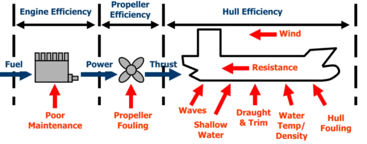
From these formulas and extra notes from the ISO 19030-1:2016 (2016), we can deduce the most important factors for our model. The primary factors are the Speed Through Water (STW) and the delivered power, which we will call Shaft Power (SP). Secondary, environmental factors include wind speed and direction, wave height and direction, swell height and direction, water depth, water temperature and density. Spectrum characteristics of the wave and swell are out of the scope of this research and will not be discussed. Relevant secondary, operational factors include draft, trim, rudder angle and the frequency of rudder movements. Secondary factors addressing the quasi-propulsive efficiency such as propeller efficiency and hull efficiency will be

(23)

Figure 2.1: Ship Powertrain (Pedersen, 2014)

seen under the term fouling. As visualized in Fig. 2.1, in order to predict the Fuel Oil Consumption (FOC), one needs information concerning the Engine Efficiency (EE). We will discuss the expected effects of these secondary factors in further detail in the following subsections.

2.1 Wind

To estimate the added wind resistance Rwi we will base ourselves on the model of

Fujiwara et al. (2006) in its simplified form as used by Gillis (2017):

Rwi= Cx(θwind,rel)qaAF (2.5)

where

Cx = the added wind resistance coefficient

θwind,rel = the relative wind direction

qa = 1₂ρairV_wind2

Vwind = the relative wind velocity

AF = the frontal ship area

For our model, this means that only the wind direction, the wind speed and the air density are needed to estimate the added wind resistance since all other factors remain constant per ship. This was also concluded by Gillis (2017) and validation for this can be found in ‘Estimating the Wind Resistance of Cargo Ships and Tankers’

(24)

by Wilson & Roddy (1970). Further, it is worth noting that much more complex models exist to estimate the added wind resistance (Ueno et al., 2012). Since wind resistance is only a secondary factor and in order to avoid making it too complex for the ML model, the authors believe that the factors Wind Direction and Wind Speed should suffice to model the effects of added wind resistance.

2.2 Waves

As mentioned by Lu et al. (2015) multiple methods exist to predict the Added Wave Resistance Rwa, with the most prominent ones being: Salvesen Method, Fuji-Takahashi

method, Kuroda-Tsujimoto-Fujiwara-Ohmatsu-Takagi method and Gerritsma and Beukelman’s method. In Gerritsma and Beukelman’s method (Gerritsma & Beukelman, 1972) the Rwa is expressed as follows:

Raw= −kcos β2 2ωe Z L 0 bs|VZb| 2_x b (2.6) where

Raw = the added wave resistance

k= the wave number β = the heading angle

ωe = the frequency of encounter

L= the ship’s water line length

|V_Z_b|= the amplitude of the velocity of water relative to the ship

bs = the sectional damping coefficient

xb = is the x coordinate on the ship

It is also found that a simplified version of Gerritsma and Beukelman’s method by Alexandersson (2009) yields a comparable accuracy, without using the complicated strip theory (Lu et al., 2015).

Another formula to calculate the average resistance of waves to the total resistance has been used by ISO 15016:2015 (2015); Luo et al. (2016) and formulates Raw as

(25)

Chapter 2. Factors influencing Speed Through Water (STW) follows: Raw = 2 Z ∞ 0 Z 2π 0 ( Raw(ω, θwave,rel) ζ2 )Sζ(θwave,rel, ωr)dθwave,reldω (2.7) where

Raw = average added wave resistance

Raw(ω, θ) = ship response

ζ = wave height

Sζ(θwave,rel) = directional wave spectrum

θr = relative direction

ω = wave frequency

In conclusion, the most important factors to estimate the added resistance due to waves are the wave number, the relative direction, the frequency and the height of the waves. Other factors are ship specific or related to the spectrum characteristics.

2.3 Swell

We make a distinction between wind-waves, which was covered in 2.2, and swell. Swell is also a type of wave but is not originated by local wind, but by distant weather systems (Wikipedia contributors, 2020). Swell generally has a longer wavelength than wind waves. This leads to the possibility of wind-waves and swell being present at the same time but in different directions and magnitudes. Therefore they are measured and treated separately. The formulas mentioned in 2.2 for wind-waves also apply to swell, thus the most important factors to take into account are relative swell direction, swell height and swell frequency.

2.4 Water Depth

An explicit representation of water depth as a part of the total ship resistance can be found in (K. Wang et al., 2018). The authors present a varying formulation of total ship resistance based on the same underlying theories (Holtrop & Mennen,

(26)

1982; Kwon, 2008; Townsin, 2003). Total ship resistance can then be written as follows:

Rship= RT + Rwave+ Rwind+ Rshallow (2.8)

where

Rship = total ship resistance

RT = total hydrostatic resistance

Rwave = wave adding resistance

Rshallow = shallow water resistance

More specific research by Patel & Premchand (2015) shows the ranges for which the water depth affects the ship and its efficiency (Table 2.1).

Classification Range Effect on Ship

Deep Water h/T >3.0 No effect

Medium deep 1.5 < h/T < 3.0 Noticeable Shallow water 1.h/T < 1.50 Very significant Very shallow water h/T <1.2 Dominates motion

Table 2.1: Effect of water depth (Patel & Premchand, 2015) where

h = the depth of water T = the draft of the ship

In conclusion, the effect of water depth or shallowness is not present when sailing in open waters.

2.5 Water Temperature Salinity

The water temperature and salinity have a profound impact on the water density and viscosity, which in turn have an impact on the total water resistance (Gillis, 2017; Pedersen, 2014). The kinematic viscosity of seawater can be written in function of

(27)

water temperature and salinity (Bertram, 2011):

v= 10−6(0.0014s + (0.000645t − 0.0503)t + 1.75) (2.9)

and for seawater density ρ:

ρ= 1027 + [−0.15(t − 10) + 0.78(s − 35)] (2.10)

where

s= salinity expressed in parts per thousand (default value = 35‰) t = seawater temperature in °C (default value = 15°C)

v = kinematic viscosity ρ = seawater density

It can be deduced that an increase in salinity leads to an increase in kinematic viscosity and thus to a slight increase in total water resistance. For temperature, the opposite is found to be true. The higher the temperature, the lower the resulting frictional resistance. To support this Pedersen (2014) found that the difference in frictional resistance between sailing in 0°C and 30°C amounts to 7%. Confirmation of this can be found ‘Effect of Fluid Density On Ship Hull Resistance and Powering’ by Festus & Samson (2015). The authors find that increased water density results in increased hull resistance. Since water density increases with a lower temperature and a higher salinity according to the general gas law (P V = nRT ), this is in line with our expectations. In conclusion, we can say that water temperature and salinity have opposite effects on the total resistance of a ship, but it is expected that the effect of temperature will be more noticeable than salinity (Gillis, 2017).

(28)

Figure 2.2: Worldwide salinity map (Kostis, 2009)

2.6 Draft & Trim

Draft and trim are measurements related to how the ship is positioned in the water. They vary depending on many factors. As can be seen in fig 2.3, the draft of a ship

TM is how deep the hull of the ship lies below the waterline at the center of flotation

F. The trim is defined as the difference between the draft forward TF and the draft

aft TA. If the waterline would be represented by W0− L0, the trim would be zero

since TF = TA. If however the waterline would be represented by Wθ− Lθ, the trim

would be a positive value equal to TF − TA. In layman terms, the trim of a ship

can be described as how tilted the ship lies in the water, as seen by its length-axis. The trim and draft of a ship can change depending on loading conditions, seawater density, speed, etc.

There has been plenty of research regarding the effect of trim and draft on operational efficiency using tow tank testing or Computational Fluid Dynamics (CFD) (Shivachev et al., 2017; Sherbaz & Duan, 2014; Islam & Soares, 2019). The optimal trim angle for a ship depends on the draft and the speed of the ship (Islam & Soares, 2019) and suboptimal trim angles can result in resistance increases of several percentage points

(29)

Figure 2.3: Draft and Trim of a ship (Biran & Pulido, 2013)

(Shivachev et al., 2017). These optimal conditions vary per ship, but since our model is ship-specific there is no need to provide ship-specific characteristics. Providing the parameters draft and trim should allow our ML model to interpret the effect of different loading conditions since other influencing factors like ship speed and water density will also be taken into account.

2.7 Rudder Angle & Variability

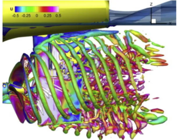
The powering requirements of a ship are influenced by the interaction effects between a ship’s rudder and propeller (Badoe et al., 2012). Much high-computational research has been done to model these complex interaction effects (Mofidi & Carrica, 2014; Felli et al., 2009). Some even state that the end-to-end process of simulating these effects for a certain geometry “can take 4 months of a highly trained engineer” (Mofidi & Carrica, 2014). Since this kind of complexity falls out of the scope of this research, we believe a simpler approach is appropriate.

Bertram (2011) states that rudders have minimal impact on resistance in the neutral position and can even improve propulsion, while moderate rudder angles may already increase resistance by a considerable 2-6%. In conclusion, we believe that simply providing the ML model with rudder angles and rudder variability over time should

(30)

Figure 2.4: Visualization of the complexity of the interaction effects between propeller and rudder (Mofidi & Carrica, 2014)

allow the model to partly capture this complex relationship between rudder angles and resistance.

2.8 Engine Efficiency (EE)

As visualized in Fig 2.1 we can write Fuel Oil Consumption (FOC) as follows:

F OC = ShaftP ower × EngineEfficiency (2.11)

Engine Efficiency (EE) however is a very hard parameter to model and/or measure (M. Schultz et al., 2011). Other research assumes EE to be a constant since the state of a diesel engine is expected to change very slowly over time and if sudden changes occur, these are expected to be handled immediately (Adland et al., 2018; Gillis, 2017). Adding further to this uncertainty is the fact that this formula assumes that the same type of fuel is used over time, which is usually not the case. In order to correct for this variability detailed information regarding the type of fuel used is necessary which is often not available. In conclusion, this research will also consider EE to be a constant. However, it is crucial to bear in my mind the possible variability that is discarded by making this assumption.

(31)

Figure 2.5: A ship in fouled condition (Mfame, 2016)

2.9 Fouling

2.9.1 Definition

Marine growth or marine fouling can be described as organisms accumulating on surfaces beneath the waterline, such as the hull or the propeller of a ship (Bressy & Lejars, 2014). According to Bressy & Lejars (2014) “bacteria, diatoms, and algae spores are the main micro-organisms which settle on ship hulls, while barnacles, tubeworms, bryozoans, mussels, and algae are the most common macro-organisms”. Globally more than 4000 different types of marine biofouling have been identified (Simberloff & Rejm´anek, 2011). The primary consequence of fouling is the substantial increase in drag resistance of the ship (Adland et al., 2018; Lu et al., 2015; Munk et al., 2009; Owen et al., 2018; Townsin, 2003). This, in turn, requires the ship to use more power to achieve the same speeds, which leads to increased fuel consumption (Munk et al., 2009; M. Schultz et al., 2011). Another negative consequence of fouling is the possibility of transferring invasive aquatic species and thus disrupting ecosystems (Uzun & Yigit Kemal Demirel, 2019). Marine biofouling has been identified as a primary economic and ecological concern by the International Maritime Organization (IMO). An example of Marine Fouling on the hull and propeller of a ship can be seen in Fig. 2.5.

(32)

2.9.2 Influencing Factors

The settlement of fouling evidently increases in time (Adland et al., 2018; Cao et al., 2011), but other factors also play an important role in determining its growth rate. A non-exhaustive list given by Uzun & Yigit Kemal Demirel (2019) includes water temperature, salinity, pH, nutrient abundance, the velocity of water flow, water depth and solar radiation as environmental factors. A list of physical factors derived from the surface properties of the ship includes micro-texture, surface charge, wettability, roughness, colors and contours (Uzun & Yigit Kemal Demirel, 2019; Bressy & Lejars, 2014). All these physical factors are closely related to the coating of a ship, which will be discussed in 2.9.3. Operational characteristics such as the average speed and the duration of idle times play a crucial role, since fouling organisms can normally not attach to ships traveling above 4-5 knots (Anoman et al., 2017). Therefore, ships that are often idle for longer periods are much more prone to fouling. In conclusion, we can say that there is an abundance of factors that influence the characteristics of marine fouling for a particular ship, making it a very complex topic.

2.9.3 Antifouling Coatings

Antifouling coatings play a central role when it comes to marine fouling. These special paints are applied to the hull of the ship in an attempt to prevent the growth of fouling. Next to fouling prevention they also limit surface deterioration (Adland et al., 2018). There are multiple types of coatings, yet the most important distinction is between biocidal and non-biocidal coatings (Uzun & Yigit Kemal Demirel, 2019). Biocidal coatings include Self-Polishing Copolymers (SPC) and Controlled Depletion Polymers (CDP). These coatings function by releasing chemically active elements that prevent the attachment of organisms. In the past SPC’s used a tributyl tin (TBT)-based biocide and were the preferred antifouling coating (Munk et al., 2009). However, TBT-based compounds were officially banned in 2001 by the IMO due to their ‘adverse effects on non-target maritime organisms’ (Bressy & Lejars, 2014). With increasing regulatory measures for biocidal coatings, more attention is being drawn to non-biocidal coatings such as Foul Release Coatings (FRC) (Bressy & Lejars, 2014). FRC’s are better for the environment since they do not contain toxic components (Uzun & Yigit Kemal Demirel, 2019). FRC’s possess a unique

(33)

structure that minimizes the attachment strength between the hull and the fouling organisms. These organisms are then automatically removed by the hydrodynamical stress experienced during navigation at high speeds (> 15 knots) (Bressy & Lejars, 2014; Uzun & Yigit Kemal Demirel, 2019). This can result in a sudden decrease in frictional drag once these high speeds have been achieved. In conclusion, it is crucial to know what type of antifouling coating is used before we compare models, since the evolution of fouling is drastically different depending on it.

2.9.4 Measuring Fouling

Measuring fouling is a very difficult topic and lacks standardization. Since there are numerous types of fouling species and these can all occur in varying degrees, it is almost impossible to use a standardized metric to express this. This is a known issue in the academic community (Pedersen, 2014; Townsin, 2003). Furthermore, measuring fouling is not per se useful since it has been observed that the relationship between the fouling rate and drag resistance is highly nonlinear and extremely complex (Kempf, 1937; M. Schultz et al., 2011). Adding to this complexity is the fact that the relationship between fouling rate and drag resistance not only depends on the type of fouling, but also on the design of the ship. In conclusion, a standardized measurement for fouling is practically impossible and even if it were possible it would not yield the desired results.

2.9.5 Quantifying the effect of Fouling

As mentioned before, the primary consequence of marine fouling is the resulting increase in drag resistance. This requires an increase in engine power to achieve the same speeds and thus an increase in fuel consumption. Several studies have attempted to model or measure this effect with varying results (Kempf, 1937; Seo et al., 2016; Lu et al., 2015; Munk et al., 2009; Owen et al., 2018; M. Schultz et al., 2011; M. P. Schultz, 2007; Townsin, 2003). Cross-study comparability is challenging due to multiple reasons (Owen et al., 2018). Different metrics are used to express the fouling rate. Periods of different lengths were used for research. Some studies research fouling in general, while others look specifically at hull fouling or propeller fouling. Some studies monitor the change in fuel consumption, while others monitor the change in

(34)

delivered engine power, Speed Through Water or drag resistance. Furthermore, every ship reacts differently to fouling depending on their ship design. Finally, reflecting on all the possible factors that influence fouling mentioned in 2.9.2, it is evident that all these studies were performed under varying conditions and therefore are not comparable. We can however use the results of these studies to better understand the possible magnitude that fouling might have on a ship’s efficiency. In a well-respected study by M. P. Schultz (2007) it is stated that the drag resistance is increased by 2%-80%, depending on the type of fouling for a certain ship. Another study of 32 vessels over 48 dry-docking intervals by Krapp & Vranakis (2013) found that the average efficiency loss due to hull and propeller performance was between 11-18%. The same study found that 5 years after the last dry-docking the ship would require 36% more power for the same activities. It can be concluded that fouling has a considerable effect on the resistance of a ship and thus also on the power requirements and fuel consumption. However, a standard formula to calculate this factor is not available due to its complexity and lack of comparability between different ships.

2.9.6 Fouling Removal

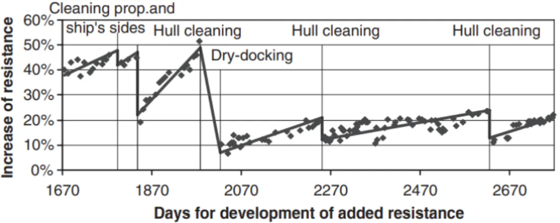
To remove fouling and its negative effects, ship operators have multiple actions they can perform. The most significant action is dry-docking, where the ship is taken out of the water to perform thorough maintenance. This is performed on average every 2.5-5 years and can cost up to millions of dollars for large vessels (Munk et al., 2009). Hull cleanings and propeller polishing are performed in between dry-docking. These smaller actions can be performed while the vessel remains in the water and aim to recoup some of the efficiency losses. Hull cleaning and propeller polishing cost between $10000-$30000 and $2000-$5000 USD respectively (Munk et al., 2009). A case study of how these actions can affect efficiency can be observed in Fig. 2.6. As displayed by Munk et al. (2009), the left side of Fig. 2.6 shows a ship with a depleted antifouling layer. As a consequence, the efficiencies gained by hull cleaning quickly evaporate, as indicated by the steep slope. After dry-docking a substantial decrease of 40% in resistance was achieved. Because of the new layer of anti-fouling applied during dry-docking, the efficiency gains created by further hull cleanings last much longer, as indicated by the moderate slope. The removal of the antifouling layer

(35)

Figure 2.6: Effects of fouling removal (Munk et al., 2009)

is accelerated by hull cleanings using hard brushes, which are necessary to remove larger fouling organisms. This will lead to an increase in resistance growth after the hull cleaning with hard brushes. To counter this Munk suggests performing hull cleanings before the slimy layer of bacteria has turned into a layer of larger organisms that requires hard brushes. This stage corresponds with 12% added resistance after dry-docking. In this preliminary fouling stage, it is possible to perform the hull cleaning with soft brushes that leave the antifouling layer undamaged. This strategy results in a longer life cycle of the expensive antifouling layer but requires an accurate method to estimate the level of fouling.

2.9.7 Followed approach to model Fouling

Considering the economic importance and the inherent complexity of fouling, it is believed that ML is an ideal technique to solve this issue (Coraddu et al., 2019; Leifsson et al., 2008; Pedersen, 2014). Theoretical models are not able to capture the complexity and variability of fouling effects due to a multitude of reasons mentioned in 2.9.5. One of the main issues is the variability between ships. Even if an appropriate theoretical model were found for a certain ship, it would only work for that particular ship design and coating. By using ML, a new model can be created for every unique ship without consuming too many resources and time while maintaining acceptable accuracy. In our approach we will not aim to model fouling explicitly as there are no standardized measurements for fouling. Rather we will model the efficiency loss of a ship due to fouling. This can be done by modelling the efficiency loss in operational

(36)

metrics such as Speed Through Water, Engine Power or Fuel Oil Consumption. To model this efficiency loss our approach first aims to model the expected Speed Through Water (STW) for a ship that is unfouled, based on input variables such as shaft rotations per minute (SRPM), trim, draft, weather conditions, etc. It can be guaranteed that a ship is unfouled by using data just after the ship left dry-docking. Once a model is available that can accurately predict the STW given the necessary input variables, we can compare the predicted value for STW to the actual, measured value of STW. In the first months, we expect the predictions of the ML model to fall in line with the actual values of STW. After several months or years, we expect a certain level of fouling to occur. Since the level of fouling is not an input variable in our model, it will not be able to correct for this fouling factor. As a result, it is expected that our model will consistently predict higher STW values than the actual measured STW, since the fouling is slowing the ship down compared to unfouled conditions. Assuming that all other relevant factors are given as input variables and having a high enough accuracy, we can conclude that the difference between the predicted STW and the actual STW is the consequence of fouling. The same method can be applied to Engine Power (EP) or Fuel Oil Consumption (FOC). This approach by Glaessgen & Stargel (2012) is called ‘Digital Twin’ as it compares the actual values of the ship to the expected digital values of the ship according to the model. This technique has been used by (Coraddu et al., 2019; Gillis, 2017; Pedersen, 2014).

FV =

Vobserved− Vmodel

Vobserved (2.12)

where

FV = fouling rate based on speed loss due to fouling

Vobserved = measured speed through water

Vmodel = modeled speed through water in clean state

As a result, this process consists out of two parts. The first aims to accurately predict the STW based on an extensive set of input variables using ML, given data from an unfouled ship (Chapter 3, 4, 5, 6). The second part explores how this ML model

(37)

can be used over time to predict the efficiency loss due to fouling of this same ship (Chapter 7).

(38)

(39)

Chapter 3

Literature Study on Modeling

the STW of a ship

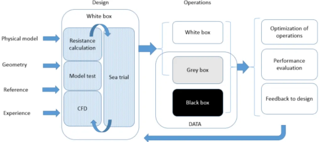
In this section, the techniques and results of former studies trying to model STW/EP/FOC and possibly fouling are summarized. A distinction is made between white box, grey box and black box approaches. White Box Models (WBM) are based on physical knowledge of the process and are theoretical, while Black Box Models (BBM) are based on empirical, historical data using statistical inference techniques such as ML (Coraddu et al., 2019; Gillis, 2017; Haranen et al., 2016; Pedersen, 2014). A Grey Box Model (GBM) is a hybrid between a WBM and a BBM and aims to combine the strengths of both approaches in order to achieve an even better accuracy (Haranen et al., 2016; Leifsson et al., 2008). The approach followed in this research is a BBM. An overview by Haranen et al. (2016) of how these methods are related is given in fig 3.1.

(40)

Chapter 3. Literature Study on Modeling the STW of a ship

Figure 3.1: Overview of different modeling techniques (Haranen et al., 2016)

3.1 White Box Models (WBM)

An abundance of purely theoretical models is available to model the operational efficiency of a ship (Holtrop & Mennen, 1982; ISO 19030-1:2016, 2016; Kwon, 2008; M. P. Schultz, 2007). Apart from these classical theoretical models, another type of WBM called Computational Fluid Dynamics (CFD) has emerged (Seo et al., 2016; Owen et al., 2018; Song et al., 2020). CFD is also based on theoretical formulas but uses supercomputers to simulate the behavior of the fluids. This allows it to overcome some of the theoretical limitations in the other models (Song et al., 2020). The advantage of a WBM is the insight it gives into the problem being modeled (Haranen et al., 2016). It allows the user to understand what factors have what effect on the predicted variable. An extensive list of reasons why a WBM is not ideal for fouling estimation can be found in Haranen et al. (2016). Additional reasons why these models are not considered the end-solution for fouling estimation can be any of the following: the model only works for one type of ship, the models require a vast number of ship-specific parameters and large computational resources (CFD), the model is too general to achieve the required accuracy (Lu et al., 2015), the model mistakenly assumes fouling to be only dependent of the time factor, the model does not consider fouling at all or does not include other relevant factors.

(41)

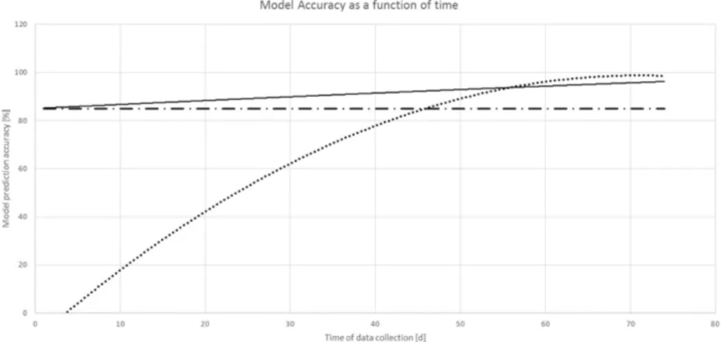
Figure 3.2: Accuracy of different modeling techniques (Haranen et al., 2016) -WBM (dash-dot), GBM (solid), BBM (dot)

3.2 Grey Box Models (GBM)

GBM’s offer the advantage of WBM’s of being able to make predictions based on theoretical insights from day one. As more operational data becomes available, black box techniques can be used to continually improve the accuracy of the GBM (Haranen et al., 2016). According to Haranen et al. (2016) GBM’s produce more reliable predictions for uncommon conditions like storms, than BBM’s, since BBM’s might have no prior knowledge to fall back on. This is the case when only a limited amount of data is available and not all possible conditions have been experienced before. Previous studies using GBM’s to predict the effect of fouling on operational efficiency include Coraddu et al. (2017); Haranen et al. (2016); Leifsson et al. (2008); Uzun & Yigit Kemal Demirel (2019). These studies achieved accurate results, but as Fig 3.2 by Haranen et al. (2016) shows, it has been proven that given several months of training data, BBM’s outperform GBM’s. Given this limited time frame where GBM’s outperform BBM’s, the authors of this research believe that BBM’s are the best approach to obtain an accurate model for fouling.

3.3 Black Box Models (BBM)

As Fig 3.2 illustrates, given enough training data, BBM’s outperform WBM’s and GBM’s. As a result, the remainder of this research focuses solely on BBM’s, often

(42)

called Machine Learning (ML) models. However, it is important to stress the most prominent disadvantages of using ML once more. The first is the black box-nature of these models that limits the user from explicitly modeling the relationships between the input variables and the dependent variable. Further, the quality of an ML model is highly dependent on the quality of the given data. This is often referred to as Garbage In, Garbage Out (GIGO). Next to the quality of the data, the amount and variability of the data also play a crucial role. ML models require large amounts of data with sufficient variability in order to generate accurate predictions, since it learns from past situations. Nevertheless, when used for the right problems and taking the mentioned limitations into account, ML can prove extremely valuable. Since the problem at hand is an extremely complicated phenomenon, almost impossible to model using theoretical formulas, and considering the vast amounts of high-quality data that ships generate, the authors believe ML to be a fitting technique.

Due to the numerous amounts of statistical techniques available, there are endless modeling possibilities. Attempts to model the operational efficiency of a ship and the effect fouling using ML include Be¸sik¸ci et al. (2016); Coraddu et al. (2019); Gillis (2017); Gkerekos et al. (2019); Haranen et al. (2016); Pedersen (2014); Petersen et al. (2012); S. Wang et al. (2018). Gillis (2017) used Random Forest Regression and did not arrive at conclusive results due to a lack of qualitative data. Pedersen (2014) applied Neural Networks and Gaussian Process Regression to predict energy consumption. The model is then used to detect maintenance events such as hull cleaning. Petersen et al. (2012) use a tapped-delay neural network. In their research lagged dependent variables are given as input variables. Even though this should drastically decrease the difficulty of achieving high accuracy, their results are only similar or even worse compared to those of other studies. Their model is then deployed for a trim optimization problem. Be¸sik¸ci et al. (2016) apply neural networks to predict the Fuel Oil Consumption of a ship. They use shaft RPM as an input variable, next to other factors such as speed, draft, trim and weather conditions. It should be noted that this is a questionable approach since there is a direct relationship between the shaft RPM of an engine and the fuel consumption of that same engine. As a result, it does not make sense to take additional factors such as trim, draft

(43)

and weather conditions into account, since the relationship between shaft RPM and FOC remains unchanged, independent of those conditions. The authors use their model to develop a decision support system. Coraddu et al. (2019) employ a Deep Extreme Learning Machine (DELM), which is also a neural network, to predict the speed loss due to fouling using the Digital Twin approach. They then compare its accuracy to a WBM proposed by ISO 19030. Since they do not explicitly mention any accuracy metrics for their DELM model and do not mention that they made a train-test split, it is impossible to interpret the results of their model. Haranen et al. (2016) use Multivariate Adaptive Regression Splines (MARS) in combination with bagging to model speed loss and power loss. Accuracy measures for their models are not provided. A first comparative study of machine learning techniques to predict fuel oil consumption has been performed by Gkerekos et al. (2019). They deployed Linear Regression, K-Nearest Neighbours, Decision Tree Regressors, Support Vector Machines, Random Forest Regressors, Extra Tree Regressors, Neural Networks and ensemble methods and compared the results. It should be noted that for the ships V1 and V2 that they apply the model to, only 745 and 768 data points were available after pre-processing. A valid train-test split, model tuning and K-fold cross-validation were performed. They conclude that the best results were obtained from ETR’s, ANN’s and RF, followed by SVR. They obtained an impressive R2 _{of 90% or more}

for some models. It is also concluded that using data obtained from automated data logging using on-board sensors increased the R2 _{by 5-7%, compared to models}

using noon data. A comparative study by S. Wang et al. (2018) shows the potential of LASSO-regression compared to Neural Networks, Support Vector Regression and Gaussian Processes. It should be noted that no explicit mention of model tuning is made for the NN, SVR GP, which might suggest that this step is omitted in the research. This would explain the surprising outperformance of LASSO-regression compared to the other methods. Summarizing, we can say that the research by Pedersen (2014) and Gkerekos et al. (2019) is the most relevant since it respects basic ML-modeling truths while not omitting crucial details concerning accuracy metrics or tuning approaches. Different studies have modeled different dependent variables. As Adland et al. (2018) mentioned, this leads to the inability of comparing results over studies and techniques. Pedersen (2014) attempts to model the energy

(44)

consumption of a ship, Gkerekos et al. (2019) the fuel Oil Consumption of a ship and other studies have modeled the expected speed through water of a ship or the engine power requirements. The aim of the first part of this study is to find the ML-technique that performs best for this specific problem. To do so, the most important techniques by Pedersen, Gkerekos and Wang will be researched while also researching other, newer ML-techniques that the authors deem appropriate.

(45)

Chapter 4

Overview of relevant Machine

Learning Techniques

Machine Learning (ML) is an umbrella term to describe the collection of statistical inference techniques that are able to extract insights from data without being explicitly programmed how to do so. An official definition of Machine Learning is hard to define and there has been criticism that the term ML has been used too much as a buzzword for basic statistical techniques. ML is seen as a subset of Artificial Intelligence (AI). Within ML a clear distinction is made between Supervised and Unsupervised ML. For an unsupervised problem, the training data is given and the model is assumed to extract some insight out of the training data, without explicitly being told what to look for. An example of this could be customer segmentation using clustering. Supervised ML, on the other hand, not only requires training input (independent) variables, but also training dependent variables. The aim of supervised ML is thus to create a model that uses the independent variables as input and is able to return as output predictions for the dependent variable, that are as close as possible to the actual measured values of the dependent variable. Since we have described this research as an attempt to model the STW, we can define the problem at hand as a Supervised ML problem. For Supervised ML, a further distinction is made between Classification and Regression problems. In Classification problems, the dependent variable is part of a finite number of discrete outputs. A textbook example would be classifying emails as either ‘spam’ or ‘not spam’, 1 or 0. The

(46)

Chapter 4. Overview of relevant Machine Learning Techniques

solution space of Regression problems, on the other hand, is continuous and contains endless possibilities. As STW is a continuous variable, the problem is a Supervised Regression Problem. The following subsection will give a brief explanation of crucial statistical concepts such as the quality of fit of a model and bias and variance. In the remaining subsections, an overview of possible ML techniques for Supervised Regression will be given. A short explanation of their workings will be given, as well as their strengths and weaknesses. Every subsection will be concluded with how we expect the specific ML technique to perform for our particular problem, based on its inherent strengths and weaknesses. The ML models are also divided in Frequentist and Bayesian approaches.

4.1 Modelling Fundamentals

To facilitate the comparison of ML techniques, we will briefly discuss some standard ways to represent a model. For now, we will disregard the validation set and only consider the train and test set. Every data set for Supervised ML consists of independent variables Xi and a dependent variable Y . As a consequence we can write a pair of

independent variables and their dependent variable as (Xi, ninputs, Yi). Furthermore,

the complete data set D, consisting out of all the pairs E(Xi, ninputs, Yi), is split up

into two parts. Often 70% of the pairs are grouped together and called the ‘training set’, while the remaining 30% is also kept together and called the ‘test set’. These percentages can vary but usually are in these ranges. Depending on the type of data, this split can happen arbitrarily or has to follow certain rules to prevent ‘leakage’ between the train and test data. Then using a chosen ML technique, a model is trained using the train set. Using the XN of the train set as input variables and

given the Yi of the train set as desired output, the model trains itself to find a

general relationship between the Xn and Y , so that for every (Xi, ninputs, Yi) the

value predicted by the model ˆYi is as close as possible to the actual value Yi. How

‘close’ these values are to each other can be expressed in multiple ways. The metrics used for this purpose are called metrics for goodness of fit and measure how well the model performs. We will discuss these metrics in 4.1.1. After the model is trained using the train set, it is applied to the test set. The model receives Xi as input from

(47)

set. The model must rely on the relationships it learned in the training set, to make predictions for these new, unseen input variables Xi of the test set. These predictions

ˆ

Yi made by the model are then compared to the actual values for Yi of the test set

using metrics for goodness of fit. The reason why a separate train and test are used is to prevent overfitting, a topic that will be further discussed in 4.1.3.

4.1.1 Goodness of Fit

4.1.1.1 Determination Coefficient R2

R2 is the best-known metric for goodness of fit and can be written as:

R2 = 1 − Pn i=1(Yi− ˆYi)2 Pn i=1(Yi− Yi)2 (4.1) where Yi = actual value ˆ Yi = predicted value Yi = average value of Yi

This metric can be interpreted as the proportion of the variation of Y which is explained by the model (Li & Wang, 2019). The advantage of this metric is that it is easily interpreted and ensures cross-study comparability since it is standardized. The biggest disadvantage, however, is that it is only valid for linear models. For non-linear models, the decomposition that R2 _{is based on, is no longer valid (Li &}

Wang, 2019). As discussed later on, the problem in this research is of a non-linear nature, so R2 _{is not a valid metric. However, in reality, we often see the misuse of R}2

for non-linear models. This is the case in the research by Gkerekos et al. where R2 _is

the main metric used. Although, R2 _{is theoretically not valid for non-linear models,}

it still gives an indication of goodness of it and since we want to ensure comparability over studies, we will also be reporting the R2 _{of our models. However, it is important}

to know that this metric is fundamentally flawed for non-linear models and that is why this research will focus mainly on the metrics MAE and MAPE.

(48)

4.1.1.2 Mean Absolute Error (MAE)

The Mean Absolute Error is calculated as follows:

M AE(Y, ˆY) = 1 n n X i=1 |Yi− ˆYi| (4.2)

MAE has the advantage of being easily interpretable since it is expressed in the same unit as the dependent variable and according to the same scale, unlike the Mean Squared Error (MSE). It is also more robust to outliers than the MSE. There also no theoretical flaws in this interpretation, unlike R2_s_{. The only disadvantage is that}

MAE is not a standardised metric and can not be compared over studies or different data sets.

4.1.1.3 Mean Absolute Percentage Error (MAPE)

MAPE is a variant of MAE and is computed as follows:

M AP E(Y, ˆY) = 1 n n X i=1 |Yi− ˆYi Yi |.100% (4.3)

Compared to MAE, MAPE has the advantage of being standardized. It still maintains the advantage of being easily interpretable. The disadvantages of MAPE, however, are that it is dysfunctional when some values of Yi are zero and that it has an inherent

bias of promoting undervalued estimations (Gkerekos et al., 2019). 4.1.1.4 Mean Bias Error (MBE)

The mean bias error is written as follows:

M BE(Y, ˆY) = 1 n n X i=1 (Yi− ˆYi) (4.4)

It is a simplified version of the MAE where overestimations and underestimations cancel each other out. This metric is used to identify if a model, on average, underestimates or overestimates compared to the true values. It is thus a way to capture the direction and quantification of the bias of a model. Unbiased, accurate

(49)

models are expected to have an MBE equal to zero. This metric will become crucial in the Digital Twin approach followed in this research.

4.1.1.5 ”Chi-by-eye” Visualization

All numerical assessments of goodness of fit are eventually flawed one way or another. An alternative approach is to visualize your results and interpret those visually. This considerably less scientific approach can not be expressed numerically, but often allows the researchers to understand the model and its flaws much better than numerical metrics. It is sometimes referred to as “Chi-by-Eye”.

4.1.1.6 Conclusion Goodness of Fit

After comparing the strengths and weaknesses of the different metrics, it is concluded that for this research MAE will be used as the primary metric for Goodness of Fit. MAE has no inherent bias and is easily interpretable. Further, it is robust to outliers which is favourable since the sensor data we are using is known to contain measurement errors. To ensure comparability over different studies and data sets, standardized metrics such as R2 _{and MAPE will also be reported. It is however}

important to remember the inherent flaws of these two metrics, as mentioned above. Finally, the MBE will also be reported due to its significance for fouling detection.

4.1.2 Bias and Variance

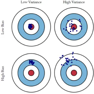
Next to metrics for goodness of fit, bias and variance are two more crucial concepts in order to understand the quality of a model. Bias is defined as the error as a result of wrong assumptions by the model, while variance can be described as the error due to oversensitivity to fluctuations in the training data. These concepts are best explained through examples and visualizations. The difference between variance and bias is intuitively explained in fig 4.1. The ideal model thus has a low variance and a low bias. However, while optimizing the model, it is often experienced that decreasing one increases the other. This trade-off is known as the bias-variance trade-off and is a key challenge for every ML problem.

In a situation where the bias is relatively high, the model, on average, fails to give predictions that are in line with reality. The model is unable to find the right

(50)

Figure 4.1: Draft and Trim of a ship (James et al., 2013)

relationship between the independent variables and the dependent variable. This phenomenon of high bias is called underfitting. In a situation where the variance is high, the errors of the predictions vary widely. This is a result of the model being oversensitive to small details in the training data. As a result, the model assumes strong relationships based on the training data, that do not always hold true in reality. This phenomenon of high variance is called overfitting. It is important to note that one does necessarily exclude the other.

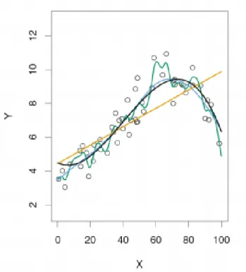
An example of the trade-off between overfitting and underfitting is visualized in fig 4.2 by Gillis (2017). We see the visualization of multiple models using X as independent variable to predict the dependent variable Y. Considering the yellow model, the straight line, we can see that is too simplistic and that it does not capture the non-linear relationship that is clearly present. This is an example of underfitting. Considering the green model, the highly non-linear model, we can see that it tracks the data points very well. However, we might note that the line is very sensitive to certain data points, in this case resulting in a graph that appears more complex than the relationship between X and Y actually is. This is called overfitting. The dark blue model is able to accurately model the relationship between X and Y, while not being overly sensitive to certain training points. This is an example of the trade-off

(51)

Figure 4.2: Draft and Trim of a ship (Gillis, 2017)

between bias and variance. The reason why overfitting is not preferable, even though it will yield better goodness of fit results for the training data, is that this model will not perform well on unseen data. This is the issue of generalization and will be explained in 4.1.3.

4.1.3 Generalization

Generalization is a term to express how well an ML model performs on unseen data, compared to its performance on the training data. Generalization can be seen as the main goal of every Machine Learning project (J. Friedman et al., 2001). An ML model is only useful if it can achieve accurate results for unseen data sets as well. To artificially test if an ML model would perform well on unseen data, the split between the training and the test set is made. As mentioned before, roughly 70% of data is used to train the model, while the remaining 30%, called the test set, is kept separate. After training the model the on training set, the model is used to make predictions using the independent variables in the test set. Since the data points in the test set were not used for creating the model, these points can be considered as unseen data. To investigate the generalization properties of a model, the goodness of fit of