National Institute for Public Health and the Environment
P.O. Box 1 | 3720 BA Bilthoven www.rivm.com
A comparison of jet fire models
for horizontal two-phase and liquid releases
Colophon
© RIVM 2012
Parts of this publication may be reproduced, provided acknowledgement is given to the 'National Institute for Public Health and the Environment', along with the title and year of publication.
E.S. Kooi
P.A.M. Uijt de Haag
Contact:Eelke Kooi
eelke.kooi@rivm.nl
This investigation has been performed by order and for the account of the Ministry of Infrastructure and the Environment, within the framework of Development of QRA Guidelines (M/620550/10/RI)
Abstract
A comparison of jet fire models for two-phase and liquid releases If a leak occurs in a pressurised pipeline with flammable liquids or gas, ignition will give rise to a jet fire. In the Netherlands, industries working with large quantities of hazardous substances are obliged to specify the minimum distance between these companies and surrounding buildings. How these distances should be calculated and which model to use, is laid down in legislation. The use of an alternative model requires approval from the Minister of Infrastructure and the Environment. The reliability, public nature and availability of the alternative model are important aspects in this assessment.
Shell model as an alternative
As commissioned by the Ministry of Infrastructure and the Environment, the National Institute for Public Health and the Environment (RIVM) has
investigated whether or not the Shell jet fire model is more reliable than the prescribed model for a specific location in The Netherlands. This turned out to be true. As a result, an important condition for using the model for permit application has been met. Other requirements, such as the public nature and availability of the model, were not part of this investigation.
The reason for comparing models was the suspicion that the use of the prescribed jet fire model might have induced unfounded salvaging
requirements. Therefore, the permit holder brought the outcomes of the legal model and the associated consequences up for discussion. With the Shell model, the distances would be 10 to 20 percent smaller. The use of the Shell model could also lead to smaller distances around other sites where two-phase and liquid jet fires determine the overall risk.
Method used
For this investigation we compared the complexity of the models and the quality of the validation. It turned out that the Shell model is derived from a larger set of data from experiments. In five selected cases the outcomes of the Shell model corresponded better to the measured values than the legal model.
Keywords:
Rapport in het kort
Vergelijking van fakkelbrandmodellen voor vloeistoffen en tot vloeistof verdichte gassen
Als een leiding met brandbare vloeistof of gas onder druk beschadigd raakt, ontstaat bij ontsteking een fakkelbrand. In Nederland zijn industrieën die met grote hoeveelheden gevaarlijke stoffen werken verplicht om aan te geven wat de minimale afstand is tussen deze bedrijven en de omliggende bebouwing. In wetgeving is vastgelegd hoe deze afstand berekend moet worden en met welk rekenmodel. Voor het gebruik van een alternatief model is toestemming van de Minister van Infrastructuur en Milieu nodig. Belangrijke afwegingen hierbij zijn de betrouwbaarheid, openbaarheid en beschikbaarheid van het alternatief.
Shell-model als alternatief
Op verzoek van het ministerie van Infrastructuur en Milieu (IenM) heeft RIVM onderzocht of het fakkelbrandmodel van Shell voor een locatie in Noord-Holland betrouwbaarder is dan het voorgeschreven model. Dit blijkt inderdaad het geval. Daarmee is voldaan aan een belangrijke voorwaarde voor een eventueel gebruik van het model bij de vergunningaanvraag. Overige aspecten, zoals de openbaarheid en beschikbaarheid van het model, vallen buiten het bestek van dit onderzoek.
Aanleiding voor de vergelijking was het vermoeden dat er door het gebruik van het wettelijke fakkelbrandmodel bij de genoemde locatie mogelijk onnodig zou moeten worden gesaneerd. De vergunninghouder stelde daarop de
uitkomsten van het wettelijke model en de daaraan verbonden consequenties ter discussie. Met het Shell-model zouden de afstanden 10 tot 20 procent kleiner zijn. Ook bij andere locaties waar het risico bepaald wordt door fakkelbranden van vloeistoffen en tot vloeistof verdichte gassen, kan het gebruik van het Shell-model leiden tot kleinere afstanden.
Werkwijze onderzoek
Voor het onderzoek zijn de complexiteit van de rekenmodellen en de kwaliteit van de validatie vergeleken. Het model van Shell blijkt te zijn gestoeld op een grotere hoeveelheid data uit experimenten. Voor vijf geselecteerde cases kwamen de uitkomsten van het Shell-model beter overeen met de gemeten waarden dan de uitkomsten van het wettelijke model.
Trefwoorden:
Contents
List of tables and figures—9
Summary—11
1
Introduction—13
2
Description of the models and their validation—15
2.1
Introduction—15
2.2
Description of the JFSH-Cook model as implemented in SAFETI-NL—15
2.2.1
Qualitative description of the model—16
2.2.2
Validation of the model—18
2.3
Description of the Barker LPG jet fire model as implemented in FRED—19
2.3.1
Qualitative description of the model—19
2.3.2
Validation of the model—20
2.4
Description of the Cracknell generic two-phase and liquid jet fire model as implemented in FRED—21
2.4.1
Qualitative description of the model—21
2.4.2
Validation of the model—22
2.5
Quantitative behaviour of the models—23
2.5.1
Definition of input variables—23
2.5.2
Results—23
2.6
Summary—27
3
Comparison of model outcomes to selected set of experimental data—
29
3.1
Introduction—29
3.2
Overview of the selected set of experimental data—29
3.3
Model outcomes for the selected release scenarios—31
3.3.1
Model outcomes for the selected LPG releases from Project AA—31
3.3.2
Model outcomes for the selected crude oil releases from BFETS (phase 2)—34
3.3.3
Model outcomes for the selected butane release from JIVE—37
3.4
Discussion of outcomes—38
3.4.1
Flame size, flame shape and flame orientation—39
3.4.2
Fraction and amount of heat radiated—40
3.5
Summary and conclusions—43
4
Extrapolation of the models—45
4.1
Introduction—45
4.2
Extrapolation to the NAM Den Helder QRA scenarios—45
4.3
Discussion of the applicability of the models for the Den Helder QRA scenarios—48
4.3.1
Flame length—48
4.3.2
Flame height and lift-off—51
4.3.3
Fraction of heat radiated and surface emissive power—52
4.4
Summary and conclusions—56
5
Conclusions—59
References—61
Annex 1
Validation of the models—65
A1.1
Data used for the validation of the DNV generic two-phase and liquid jet fire model (JFSH-Cook)—65
A1.2
Data used for the validation of the Barker LPG jet fire model—68
A1.3
Data used for the validation of the Cracknell generic two-phase and liquid jet fire model—70
Annex 2
Extrapolation of the models—75
Annex 3
Assumptions and parameter choices used for the illustration of the model behaviour—79
List of figures and tables
FiguresFigure 1 Geometry of the JFSH-Cook model in SAFETI-NL. 17 Figure 2 Flame shape for the Barker LPG jet fire model. 20 Figure 3 Flame shape for the Cracknell generic jet fire model. 21 Figure 4 Flame length as a function of the release rate. 24 Figure 5 Flame length as a function of the expanded jet velocity (release
rate 50 kg/s). 24
Figure 6 Width of the frustum tip as a function of the release rate. 25 Figure 7 Width of the frustum tip as a function of the expanded jet velocity. 25 Figure 8 Fraction of heat radiated as a function of the release rate. 26 Figure 9 Fraction of heat radiated as a function of the expanded jet velocity. 26 Figure 10 Measured flame shape (50% flame occurrence) for Project AA test
3026 compared to model outcomes. 32
Figure 11 Measured flame shape (50% flame occurrence) for Project AA test
3029 compared to model outcomes. 32
Figure 12 Measured flame shape for BFETS-2 test 1 compared to model outcomes (the zone between blue and red refers to 50% flame
occurrence). 35 Figure 13 Measured flame shape for BFETS-2 test 2 compared to model
outcomes (the orange/yellow zone between blue and red refers to
50% flame occurrence). 35
Figure 14 Measured flame shape for JIVE test 8051 compared to model outcomes (the red line marks 40% flame occurrence, light blue
60% flame occurrence). 37
Figure 15 Comparison of visible flame (upper graph) with radiant flame (lower
graph) for BFETS-2 test 1. 39
Figure 16 Fraction of heat radiated as a function of expanded jet velocity. 41 Figure 17 Comparison of calculated flame shapes for the selected NAM Den
Helder QRA scenario. 48
Figure 18 Predicted flame length for discharge rates outside the validation
range. 49
Figure 19 Lowesmith data for flame length. 50 Figure 20 Predictions for butane in comparison with observational data from
[20]. 50
Figure 21 Predicted F-values in combination with Lowesmith et al. data. 53 Figure 22 Validation of the flame length (JFSH-Cook model). 65 Figure 23 Validation of the surface emissive power (JFSH-Cook model). 66 Figure 24 Validation of the incident heat radiation (JFSH-Cook model). 67 Figure 25 Flame length in the Barker model: goodness of fit 68 Figure 26 Width of the frustum tip in the Barker model: goodness of fit. 69 Figure 27 Lift-off angle in the Barker model: goodness of fit. 69 Figure 28 Surface emissive power in the Barker model: goodness of fit. 70 Figure 29 Flame length in the Cracknell model: goodness of fit. 71 Figure 30 Width of the flame tip in the Cracknell model: goodness of fit. 72 Figure 31 Lift-off angle in the Cracknell model: goodness of fit. 72 Figure 32 Length of the jet flame as a function of release rate. 75 Figure 33 Width of the frustum tip as a function of release rate. 76 Figure 34 Fraction of heat radiated as a function of discharge rate. 77 Figure 35 Spot surface emissive power versus liquid fraction (results from
Tables
Table 1 Data used for validating the flame shape (1) in the JFSH-Cook jet
fire model. 19
Table 2 Data used for developing the Barker LPG jet fire model. 21 Table 3 Data used for developing the Cracknell jet fire model. 22 Table 4 Relevant data for selected set of experimental releases. 30 Table 5 Model outcomes for Project AA test 3026 and 3029. 33 Table 6 Model outcomes for BFETS-2 test 1 and test 2. 36 Table 7 Model outcomes for JIVE test 8051. 38 Table 8 Qualitative assessment of the goodness of fit of the selected models
with respect to flame shape, size and orientation. 40 Table 9 Summary data for the fraction of heat radiated. 42 Table 10 Description of the full bore rupture QRA scenarios for NAM Den
Helder. 46
Table 11 Input data for the selected NAM Den Helder QRA scenario. 46 Table 12 Model outcomes for the selected NAM Den Helder QRA scenario. 47 Table 13 Ratio of calculated and observed heat radiation. 67 Table 14 Composition of the gas in the JIVE project. 81 Table 15 Composition of the liquid in the JIVE project. 81 Table 16 Summary of outcomes of the JIVE project. 82
Summary
In this report three jet fire models were compared. The motivation for this investigation was a claim by the Nederlandse Aardolie Maatschappij (NAM) that the jet fire model that is prescribed by the Dutch legislation, produces outcomes that are inaccurate and overconservative for specific cases. As a result, the use of this model would have undesirable consequences for permit application and land-use planning, in particular for the NAM site in Den Helder.
The scope of this study was limited to jet fires related to mixed gaseous and liquid releases. These jet fires are most relevant for the permit application for the NAM site in Den Helder and for the land-use planning around this site. For the assessment of the consequences of such jet fires, the legislative
authorities currently prefer to use the JFSH-Cook model that is implemented in SAFETI-NL. NAM claimed however that the Cracknell model from Shell would give a more reliable prediction of the consequences of these jet fires. A third model, the Barker model from Shell, was investigated for reasons of
completeness.
The investigation which model produces the best results comprised of three parts. Firstly, the physical assumptions behind the models, the amount of validation data and the quality of the validation data were assessed. Subsequently, the outcomes of the models were compared against five relevant jet fire experiments. Lastly, the quality of the model outcomes outside the validation range was investigated by comparing the outcomes with general knowledge from literature.
The outcome of the investigation was that the Shell models produce more reliable results and that the outcomes of the JFSH-Cook model are expected to be overconservative for the considered releases. The Shell models are more sophisticated and are derived from a larger set of experimental data. When compared to realistic cases, the Shell models produced better outcomes than the JFSH-Cook model. Lastly, the model predictions of the Shell models in the extrapolated range were deemed more reliable.
Overall, the Cracknell model is expected to produce the best results for the jet fire scenarios that are deemed most relevant for the NAM site in Den Helder. When using the Cracknell model, the expected consequences of these
scenarios are more limited than when using the JFSH-Cook model. The use of JFSH-Cook model could therefore lead to restrictions for the permit application and land-use planning that are undesirable and also unnecessary from a scientific point of view.
However, legislative authorities may have other requirements for the use of jet fire models in the permit application and land-use planning, such as the availability of these models for third parties and a description of these models in the open literature. These aspects were not investigated in this study.
1
Introduction
The aim of this project is to verify a claim, made by the Nederlandse Aardolie Maatschappij (NAM), that the jet fire models in FRED™ give a better prediction of effect zones for heat radiation than the jet fire models in SAFETI-NL™. In order to verify this claim, model outcomes from FRED and SAFETI-NL are compared to experimental data. In addition to available experimental data, information on jet fire properties and effect zones in the open literature are also addressed. If NAM is right, the FRED models will give a better fit to the experimental data than the models in SAFETI-NL.
Specific attention will be paid to the release scenarios that are prescribed for the Quantitative Risk Assessment (QRA) for the Den Helder site of NAM. These scenarios involve horizontal releases of mixtures containing various
hydrocarbons varying from C1 to C9 at high pressure (40 to 80 bar) from large diameter pipes (36 to 48″). In order to verify to which extent the jet fire models can be applied to these release scenarios, a detailed description of the model assumptions and model validation is needed. If the calculated effect zones using the models mentioned above differ significantly, it must be decided which of the models can best be used for the prediction of effect zones at the Den Helder site.
This report consists of the following parts:
In chapter 2 the various jet fire models will be described. The description includes the flame geometry, the surface emissive power of the flame and the total fraction of heat radiated. The description also includes an overview of the amount of data used to design or validate the model, the validation range and the quality of the fit of the key parameters in the model.
In chapter 3 the LPG jet fire model in FRED, the generic two-phase and liquid release model in FRED and the two-phase and liquid release model from SAFETI-NL will be compared to a limited set of experimental jet fire releases for which sufficiently detailed data were available. This comparison includes two jet releases performed by Shell and three releases performed by British Gas.
In chapter 4 it will be analysed to which extent the jet fire models can be used for the QRA scenarios for the NAM Den Helder site. These release scenarios differ significantly from the experimental data used in chapter 3. More specifically, the NAM Den Helder release scenarios involve mixtures of
hydrocarbons ranging from C1 to C9 and release rates which are two orders of magnitude higher than the release rates for which experimental data are available. One Den Helder release scenario is selected for further comparison and the corresponding outcomes of the jet fire models in FRED and SAFETI-NL are presented. Subsequently, the model outcomes are compared to the reported behaviour of two-phase and liquid hydrocarbon releases in the literature. This comparison with literature will provide further insight in the applicability of the FRED and SAFETI-NL models for the NAM Den Helder QRA scenarios.
In chapter 5 general conclusions will be drawn on the applicability of the FRED and SAFETI-NL models for the NAM Den Helder QRA scenarios discussed in this report. If the calculated effect zones using these models differ
significantly, we will substantiate which model is expected to give the best prediction of the size of effect zones.
The current study only comprises an assessment of the quality of the models and the expected accuracy of the model outcomes. This does not imply that the model that is expected to give the best predictions will automatically be selected as the model that should be used for third party risk calculations for the NAM Den Helder site or for Dutch establishments with flammable
substances in general. Such a decision depends on several other factors as well, including transparency, which are not addressed in this report. Furthermore, it was decided earlier that a full bore rupture of one of the fingers of the slugcatcher had to be included as one of the QRA scenarios. The possibility of this event is currently taken as a premise and its likelihood is not further discussed in this report.
All outcomes for FRED and model descriptions for FRED apply to version 5.0.0. All outcomes for SAFETI-NL and model descriptions for SAFETI-NL apply to version 6.5.3. PHAST 6.5.3 was used for the JFSH-Cook consequence analyses in chapter 3.
This comparison was carried out by the Centrum Externe Veiligheid (Centre for External Safety) of RIVM and was commissioned by the Dutch Ministry of Infrastructure and Environment. The description of the models in FRED and the validation behind these models (see chapter 2) is largely provided by Shell Global Solutions (SGS). The description of the models in SAFETI-NL and the validation behind these models (also chapter 2) was done by RIVM together with DNV. Additional data reports were provided by GL Noble Denton (formerly Advantica) and the Steel Construction Institute. Stakeholders (notably NAM, SGS and DNV) have been invited to comment the comparison.
2
Description of the models and their validation
2.1 Introduction
The model comparison is carried out for the Barker LPG jet fire model, the Cracknell generic two-phase and liquid jet fire model and the JSFH Cook model for two-phase and liquid jet fires. The first two models are implemented in Shell FRED, the latter is implemented in SAFETI-NL.
This chapter provides a qualitative description for each of the selected models. This includes:
a description of the flame shape and orientation;
a list of parameters that determine the flame shape, orientation and fraction of heat radiated;
a qualitative description of the influence of each of these parameters; insight in the amount of data used for validation, the validation range and
the quality of the fit of the key parameters.
The use of SAFETI-NL is prescribed for establishments that are within the scope of the BEVI legislation ([1]). Therefore, the JFSH-Cook model in SAFETI-NL is regarded as the point of departure and will be discussed first. The FRED models will be discussed in section 2.3 and 2.4. A first comparison of the quantitative behaviour of the models will be presented in section 2.5 followed by a summary of the first findings in section 2.6.
2.2 Description of the JFSH-Cook model as implemented in SAFETI-NL
The two-phase and liquid jet fire model that is implemented in SAFETI-NL is described in detail in the ‘JFSH Theory Document’ on the SAFETI-NL
installation CD ([2]). The model is derived from a model published by Chamberlain ([3]) in 1987, for which modifications were proposed by Cook, Bahrami and Whitehouse ([4]) in order to account for two-phase and liquid jets. The corresponding outcomes have been validated against publicly available experimental data from Bennett, Cowley, Davenport and Rowson ([5]) and Selby and Burgan ([6]).
The model may be used for flammable substances that are two-phase or liquid after depressurisation to ambient pressure, though the user is advised to verify if the modelled release conditions are in the validation range (see section 2.2.2). For the input data, such as discharge rate and final velocity, the model depends on discharge variables that are calculated elsewhere in the software.
The two-phase and liquid model that is currently implemented in SAFETI-NL deviates from the initial proposal by Cook, Bahrami and Whitehouse ([4]). In agreement with the terminology of DNV it will nevertheless be referred to as the JFSH-Cook model.
For reasons of completeness it is noted that the implementation of the JFSH-Cook model in SAFETI-NL has restrictions that do not pertain to the
2.2.1 Qualitative description of the model
2.2.1.1 Flame shape and orientation
The flame geometry is depicted in Figure 1. The flame shape is approximated with a tilted frustum of a cone. The modelled flame shape has the following features:
The flame starts at a distance B from the orifice (along the release direction). This ‘lift off distance’ is used for vertical and also non-vertical releases.
The flame length, LB, is equal to the distance between the orifice and the
flame end (tip of the frustum at the flame axis).
The length of the frustum, RL, represents the length of the burning flame
(along the flame axis).
The width of the frustum base, W1, represents the width of the burning
flame near the orifice.
The width of the frustum tip, W2, represents the width of the burning
flame at the flame end.
θj is the angle between the release direction and the horizontal (jet angle).
α is the angle by which the flame is deflected from the release direction due to wind impact.
For non-horizontal releases, the angle between the flame and the horizontal may increase or decrease due to wind effects. For horizontal releases, the flame direction is always horizontal. In particular the JFSH-Cook model does not take into account flame lift off due to buoyancy effects. Furthermore, there is no interaction between the modelled flame and the ground. Part of the modelled frustum may have a negative z-coordinate, in which case a warning and/or error is issued.
According to the Dutch guidelines for third party risk calculation ([1]) releases from aboveground pipelines should always be modelled as (along wind) horizontal releases, for which case both θj and α are equal to 0. In the related
software tool PHAST (also owned and developed by DNV) it is possible to take into account crosswind effects on jet fires.
The flame length in the JSFH-Cook model is determined by the wind speed, the effective source diameter of the release and the Richardson number. The Richardson number represents the ratio of buoyancy and momentum forces and is proportional to the third root of the ratio g/(m•vj), in which g is
gravitational acceleration, and m•vj the momentum of the jet (derived from
Figure 1 Geometry of the JFSH-Cook model in SAFETI-NL.
The features above were already present in the Chamberlain model for gaseous releases ([3]). For two-phase and liquid releases, the following rules are defined in the JSFH-Cook model:
Following a recommendation of PHAST users in 1998, the amount of mass involved in the jet is set at three times the vapour mass after rainout (with the total release rate as an upper limit). This assumption is expected to give a better prediction of flame lengths for liquid releases but has not been verified with experiments. Note: this assumption does not apply to
the ‘stand-alone model’ which is available in PHAST. However, as the current study focuses on SAFETI-NL, the stand-alone models will not be discussed.
The effective diameter of the release is linear with (
ρ
j/ρ
sv)0.5, in whichρ
j isthe density of the jet after expansion to atmospheric pressure and
ρ
sv isthe saturated vapour density at the orifice. For pure gas releases the corresponding factor was (
ρ
j/ρ
air)0.5, ρair being the density of ambient air.According to the JFSH theory document ([2]) this gives an effective diameter that - in conjunction with the release rate - produces an expanded jet velocity that is equal to the expanded jet velocity had it been a pure gas release.
The lift off distance is equal to 1.5% of the flame length for all horizontal two-phase and liquid releases. As the release direction is equal to the flame direction (in accordance with the Dutch guidelines), the frustum length amounts to 98.5% of the flame length.
The width of the flame at the base (W1) is very similar to the width of the
frustum in the Chamberlain model ([3]). It depends on the ratio of wind speed and expanded jet velocity, the effective release diameter and the Richardson number (buoyancy versus momentum). The width of the flame at the top (W2)
is taken entirely from the Chamberlain paper, and depends on the flame length and the ratio of wind speed and expanded jet velocity.
2.2.1.2 Surface emissive power and fraction of heat radiated
The surface emissive power is derived from the total amount of heat radiated and the total surface area of the flame. For fuels with a molecular weight (MW)
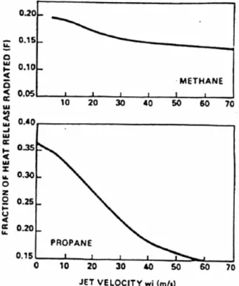
lower than 21 kg/kmol, the fraction of heat radiated is taken from the Chamberlain paper ([3]) and depends only on the expanded jet velocity. The fraction of heat radiated diminishes from 0.32 for low velocity releases, to 0.11 for high velocity releases. For heavier fuels, the fraction of heat radiated calculated with the Chamberlain correlation is increased by a factor (Mw/21)0.5,
using an upper limit of 1.69 for this factor. Overall the fraction of heat radiated may thus vary from 0.54 for heavy hydrocarbons released with low pressure, to 0.11 for methane at (very) high pressure.
The surface emissive power itself also has an upper limit, which is set at 400 kW/m2 in SAFETI-NL. If the surface emissive power is capped, the fraction
of heat radiated is decreased correspondingly.
2.2.2 Validation of the model
The JFSH-Cook model is a theoretical extension to the Chamberlain vapour jet model ([3]). In other words, the model is not based on experimental data directly. However, the model has been validated afterwards, against field data from ‘Project AA’ ([5]) and from ‘phase 2 of BFETS’ ([6]). The Project AA data involve horizontal free jets and horizontal impinging jets of natural gas and LPG. The free LPG releases are used for the validation of the JFSH-Cook model. The BFETS-2 data involve horizontal free jets and horizontal impinging jets of stabilised light crude oil and mixtures of stabilised light crude oil and natural gas. The releases of crude oil with no added natural gas were used by DNV for validation of the JFSH-Cook model.
A complete description of the validation is given in the JFSH theory document ([2]). Some difficulties were met by DNV because the jet fire model needs expanded jet velocity and temperature as input while the data reports only specify stagnant temperature and pressure. Another problem was that the composition of the crude oil could not be derived accurately from [6].
Moreover, at the time of the validation, the software (PHAST, PHAST Risk and SAFETI-NL) did not have a multi-component release model. Therefore, n-octane was used by DNV as a substitute for crude oil. Whether releases of mixtures can be accurately modelled with pure components will be further discussed in the text box ‘Accuracy of the models for releases of mixtures’ on page 27(1).
An overview of the number of releases used for the validation of the JFSH-Cook model is given in Table 1. The table also lists which stagnant pressures,
1 Based on a temperature-recovery table reported by Selby and Burgan in [6], it was estimated by RIVM
that about 10 wgt% of the crude oil consisted of C6-C8 hydrocarbons, and about 90% C9-C20. The temperature of 50% (vapour) recovery was 317°C and the temperature of 100% (vapour) recovery 345°C indicating that about half of the crude was C18-C20).
orifice diameters and release rates were used in the experiments. The table applies both to the validation of the flame shape (size and geometry) and the validation of the surface emissive power.
Table 1 Data used for validating the flame shape (1) in the JFSH-Cook jet
fire model. Released substance Number of releases used for validation Range of stagnant pressures Range of orifice diameters Range of release rates LPG (97% propane) 5 6.3 - 9.7 bar(g) drive pressure 10 - 52 mm 1.5 - 18.0 kg/s Stabilised crude oil 2 7 - 20 bar(g) stagnant pressure 14 - 18 mm 5.0 kg/s
(1) The flame shape includes the frustum length, width of the frustum base and the width of the frustum tip.
More information on the validation of the model is presented in Annex 1.
2.3 Description of the Barker LPG jet fire model as implemented in FRED
(The larger part of the text in this section was provided by Shell Global Solutions)
The Barker LPG jet fire model is implemented in FRED for two-phase releases of propane, butane and LPG. A full description of the model is provided in ([7]). The model can be applied to all releases of (mixtures) of propane and butane with a significant amount of liquid at the orifice. A warning is issued if the discharge rate or the exit velocity is outside the validation range.
2.3.1 Qualitative description of the model
Typical flame shapes observed during experimental pressurized releases of liquid LPG (propane and butane) have a flame region dominated by initial horizontal momentum followed by a flame region dominated by buoyancy. A flame shape model was developed to represent this observed behaviour consisting of a horizontal cone frustum to model the momentum dominated region attached to a tilted cylinder to model the buoyancy dominated part of the flame.
The intended application of the model is for liquid releases of LPG through an orifice or open pipe system driven either at saturated LPG pressure or a modest drive overpressure. The experimental test programme covered LPG mass flow rates up to 22 kg/s through maximum hole sizes of 52 mm.
2.3.1.1 Flame shape and orientation
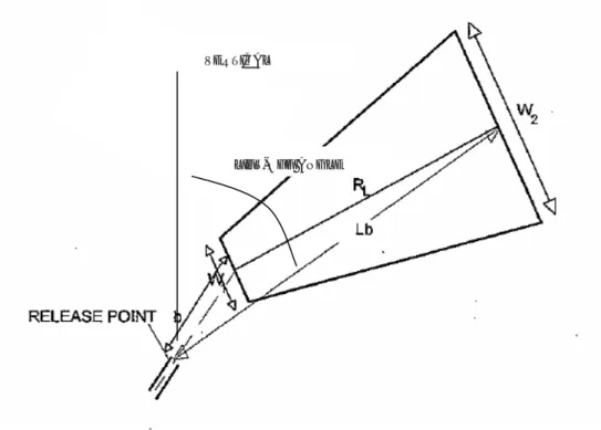
The flame of the Barker LPG jet fire model has a horizontal part shaped like a frustum of a cone, and a tilted part shaped as a cylinder. The general flame shape including orientation is displayed in Figure 2. This (two-component) flame shape represents the 50% occurrence of the flame.
Wind
cylinder
lift-off angle
Flame
width
Flame
length
Release
Figure 2 Flame shape for the Barker LPG jet fire model.
Diagram obtained from Shell Global Solutions
The flame shape is characterised by the following parameters: horizontal cone length;
width of the frustum base;
width of the frustum tip (flame width); flame length;
lift-off angle.
The horizontal cone length is determined by the exit velocity and release diameter. The width of the frustum tip is determined by mass flow rate, wind speed, release diameter and density. Increases in mass flow rate and release diameter both give wider flames. An increase in wind speed results in
narrower (and thus lower) flames. The (total) flame length is determined primarily by mass flow rate of the release. The lift-off angle is determined by the wind speed, flame width and density. In the absence of wind, the lift-off angle is roughly 60°.
2.3.1.2 Surface emissive power and fraction of heat radiated
The surface emissive power is determined by the temperature and amount of soot loading in the flame. For propane the surface emissive power is
restrained by a maximum of 230 kW/m2. For butane the surface emissive
power is restrained by a maximum of 255 kW/m2. The fraction of heat
radiated is calculated from the SEP, the surface area of the flame and the overall combustion power.
2.3.2 Validation of the model
An overview of the number of releases used for developing the Barker LPG jet fire model is given in Table 2. The table also lists which orifice pressures, orifice diameters and release rates were used in the experiments. The table applies to flame shape (geometry and size) as well as surface emissive power.
If experiments leave room for interpretation, Shell Global Solution prefers to calculate flame lengths slightly conservative, in order not to underestimate distances to heat radiation levels along the flame direction. Because flame
shape and surface emissive power are highly interdependent, this approach may sometimes result in a small underestimation of the surface emissive power.
Table 2 Data used for developing the Barker LPG jet fire model. Released
substance
Number of releases used for validation
Range of stagnant pressures Range of orifice diameters Range of release rates propane 22 small, 89 large 6.3 to 9.7 bar(g) 3 to 52 mm 0.11 to 22 kg/s butane 11 small, 15 large 4 to 20 bar(g) 3 to 52 mm 0.16 to 21 kg/s
More information on the validation of the model is presented in Annex 1.
2.4 Description of the Cracknell generic two-phase and liquid jet fire
model as implemented in FRED
The Cracknell jet fire model is implemented in FRED for general two-phase and liquid releases of hydrocarbons. A full description of the model is given in [8]. The model is applicable to all releases of hydrocarbons, including mixtures of gaseous, two-phase and liquid hydrocarbons. A warning is issued if the discharge rate or the exit velocity is outside the validation range.
2.4.1 Qualitative description of the model
2.4.1.1 Flame shape and orientation
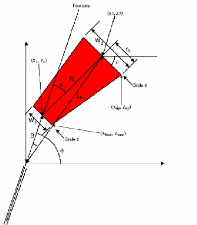
The flame of the Cracknell generic two-phase and liquid jet fire model consists of a tilted frustum of a cone and is displayed in Figure 3.
Figure 3 Flame shape for the Cracknell generic jet fire model.
Diagram obtained from Shell Global Solutions
VERTICAL
The flame shape is characterised by the following parameters: flame length (LB);
width of the frustum base (W1);
width of the frustum tip (W2);
lift-off angle.
The flame length depends on the release rate, the heat of combustion and the velocity of the wind along the release axis. The width of the frustum base is derived from the flame length and the width of the frustum tip (with a minimum value equal to the orifice diameter). The width of the frustum tip is linear with the expanded jet diameter. A further correction is applied when the released mass contains a high fraction of non-combustible products. The lift-off angle depends on release direction and expanded jet velocity, wind direction and wind speed and buoyancy. Buoyancy is determined by flame length, expanded jet diameter and gravity.
2.4.1.2 Surface emissive power and fraction of heat radiated
In the Cracknell model, the fraction of heat radiated is derived from the release rate and the expanded jet velocity. A physical argument was used to derive a correlation between the fraction of heat radiated, mass flow and exit velocity (in particular the values of the exponents in this correlation). The missing proportionality constant was subsequently deduced from experiments. An analysis described in [8] showed that the variance in the proportionality constant was limited. A conservative value was then used for the model. The correlation does not take into consideration smoke obscuration for high release rates. Therefore, the calculated fraction of heat radiated will be more conservative for high release rates.
The surface emissive power is deduced from the total flame surface area, the total combustion power of the release and the fraction of heat radiated.
2.4.2 Validation of the model
An overview of the number of releases used for developing the Cracknell jet fire model is given in Table 3. The table also lists which orifice pressures, orifice diameters and release rates were used in the experiments. The table applies to flame shape (geometry and size) as well as surface emissive power.
Table 3 Data used for developing the Cracknell jet fire model. Released
substance
Number of releases used for validation Range of stagnant pressures Range of orifice diameters Range of release rates Butane / Natural gas 27 0.6 to 4.8 barg 40 to 80 mm 2.3 to 2.7 kg/s Propylene 40 3.9 to 5.7 barg 3 to 6.8 mm 0.05 to 0.36 kg/s Kerosene /natural gas 7 0.8 to 1.4 barg 80 mm 2.4 to 2.7 kg/s Two-phase propane 22 small, 89 large 6.3 to 9.7 barg 3 to 52 mm 0.11 to 22 kg/s Two-phase butane 11 small, 15 large 4 to 20 barg 3 to 52 mm 0.16 to 21 kg/s
If experiments leave room for interpretation, Shell Global Solution prefers to calculate flame lengths slightly conservative, in order not to underestimate
distances to heat radiation levels along the flame direction. Because flame shape and surface emissive power are highly interdependent, this attitude may sometimes result in a small underestimation of the surface emissive power.
More information on the validation of the model is presented in Annex 1.
2.5 Quantitative behaviour of the models
2.5.1 Definition of input variables
It is desirable to obtain more insight in the behaviour of the three selected models. It is not feasible however, to study every detail. Therefore, specific attention is paid to those parameters that are most relevant for the size of the consequence area of the jet fire. The following parameters were used for the model comparison:
flame length;
width of the frustum tip; fraction of heat radiated.
The consequence area depends mostly on the substance released, the pressure at the orifice (or alternatively the expanded jet velocity) and the release rate (or alternatively the orifice diameter). In this section, only
releases of n-butane are discussed. Release rate and expanded jet velocity are varied.
Orifice conditions are specified as input (instead of stagnant conditions) in order to have a comparison of the jet fire models that is independent of the discharge models used. A complete overview of the assumptions and parameter choices (to be) used for the generation of the plots is given in Annex 3.
2.5.2 Results
In this subsection the quantitative behaviour of the selected jet fire models is plotted in graphs and discussed. An upper boundary of 100 kg/s is used for the discharge rate. All models are expected to be applicable in this range. In Annex 2, graphs are shown for discharge rates up to 10,000 kg/s. It is noted that the presented outcomes correspond to the inputs laid down by RIVM. The models may behave differently if other assumptions were used.
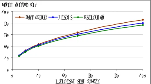
The flame length(2) as a function of the release rate is shown in Figure 4. Over the whole range (from 5 to 100 kg/s), the Cracknell model gives the lowest values and the JFSH-Cook model the highest. The gap between the two increases from 4%(3) for 5 kg/s to 11% for 100 kg/s. The predicted values by the Barker model are 4% higher than the predictions of the Cracknell model for all cases.
Figure 5 shows the flame length as a function of the expanded jet velocity for a fixed release rate of 50 kg/s. For the Barker and Cracknell models, the influence of the expanded jet velocity on the flame length is very limited. According to the JFSH-Cook model, the flame length decreases slightly with
2 In these graphs, the flame length is defined as the distance between the origin and the centre of the
flame tip.
increasing jet velocity, yielding to a total decrease of 22% over the whole range (30 to 200 m/s). Flame length (m) 0 20 40 60 80 100 0 20 40 60 80 100 Discharge rate (kg/s) JFSH-Cook Barker Cracknell
Figure 4 Flame length as a function of the release rate.
Flame length (m) 0 10 20 30 40 50 60 70 80 0 50 100 150 200
Expanded jet velocity (m/s)
JFSH-Cook Barker Cracknell
Figure 5 Flame length as a function of the expanded jet velocity (release rate 50 kg/s).
The dependence of the width of the frustum tip on the release rate is depicted in Figure 6. The Cracknell and JFSH-Cook models both show a substantial increase in tip width with increasing release rate. The Barker model shows a limited increase and has lowest predicted tip widths over the entire range (5 to 100 kg/s). For a release rate of 100 kg/s, the predictions of the Cracknell and JFSH-Cook models are roughly 100% higher than the prediction of the Barker model.
The width of the frustum tip as a function of expanded jet velocity is shown in Figure 7. According to the Barker model, the width of the frustum tip increases with increasing jet velocity. According to the Cracknell and JFSH-Cook models the tip width decreases with increasing jet velocity. The predicted values differ significantly in the lower range (Cracknell giving a four times higher value
than Barker) but tend to converge in the higher range. For 200 m/s
(corresponding to a backing pressure of about 100 bar) the predicted values by both Shell models are roughly equal, and the predicted value of the DNV model is 15 to 20% higher.
It was initially expected that the flame width would be an important parameter for the flame height and therefore for the view factor near the tail of the flame. However, in the Barker and Cracknell models, the flame height depends on the flame length, the flame lift-off angle and the flame width. Therefore, a comparison of flame width alone is not very useful.
Frustum tip width (m)
0 10 20 30 40 50 60 0 20 40 60 80 100 Discharge rate (kg/s)
JFSH-Cook Barker Cracknell
Figure 6 Width of the frustum tip as a function of the release rate.
Frustum tip width (m)
0 10 20 30 40 50 0 50 100 150 200
Expanded jet velocity (m/s)
JFSH-Cook Barker Cracknell
Figure 7 Width of the frustum tip as a function of the expanded jet velocity.
Figure 8 depicts the fraction of heat radiated (also known as ‘emissivity’) as a function of the release rate. The Barker and Cracknell models both show a decreasing emissivity with discharge rate (Barker showing the strongest decrease). The JFSH-Cook model on the other hand, predicts a constant fraction of heat radiated over the entire range (5 to 100 kg/s). For low discharge rates, JFSH-Cook predicts a fraction of heat radiated that is 26%
higher than the prediction of the Shell models. For a discharge rate of 100 kg/s, the emissivity according to the Barker model is 0.14. The emissivity according to the Cracknell model is almost 100% higher (0.27) and the emissivity according to the JFSH-Cook model 240% higher (0.47).
The fraction of heat radiated as a function of expanded jet velocity is shown in Figure 9. Again, the selected models show significantly different behaviour. The Barker model gives a constant emissivity over the entire range (30 to 200 m/s). The Cracknell model predicts a rapid decrease with increasing jet velocity and the JFSH-Cook model shows a slow decrease. The DNV model gives the highest values, being 100 to 200% higher than the values predicted by the Shell models from 50 m/s onwards.
Fraction of heat radiated
0.0 0.1 0.2 0.3 0.4 0.5 0.6 0 20 40 60 80 100 Discharge rate (kg/s)
JFSH-Cook Barker Cracknell
Figure 8 Fraction of heat radiated as a function of the release rate.
Fraction of heat radiated
0.0 0.1 0.2 0.3 0.4 0.5 0.6 0 50 100 150 200
Expanded jet velocity (m/s)
JFSH-Cook Barker Cracknell
2.6 Summary
The Barker model consists of a horizontal frustum of a cone and a tilted cylinder. It is therefore well suited for high pressure releases (giving a
horizontal jet) with high volatility (resulting in buoyancy towards the tail). The JFSH-Cook model does not include flame lift-off and will therefore not be appropriate for highly buoyant jet fires. The Cracknell model is designed to be a generic model for two-phase and liquid hydrocarbon jet fires (both buoyant and non-buoyant). This subject will be discussed in more detail in the next two chapters.
The Barker and Cracknell models are derived from experimental outcomes for two-phase releases. The JFSH-Cook model is derived from a gaseous jet fire model. Additional assumptions are used to apply the model to two-phase and liquid releases. The amount of data used to construct the Barker and Cracknell models is significantly larger than the amount of data used to validate the JFSH-Cook model. The variance in the experimental data (such as fuels used and release conditions) is also larger for the Barker and Cracknell models in comparison with the JFSH-Cook model.
Accuracy of the models for mixtures of substances with different volatilities
The jet fire outcomes depend on discharge parameters such as discharge rate and expanded jet velocity. The jet fire model in SAFETI-NL also uses the amount of rainout. In the current text box, it is described how the discharge models in FRED and SAFETI-NL deal with multicomponent discharges.
In FRED, mixtures are treated as ideal mixtures obeying Raoult’s law. In particular, mixtures are characterised by a dew point and a bubble point and the compositions of vapour and liquid are temperature dependent. It is expected that the FRED discharge models will predict the vapour and liquid fractions at the orifice well (for mixtures largely obeying Raoult’s law). As a result, they will also produce reliable inputs for the jet fire models.
In SAFETI-NL, a ‘pseudo-component’ is used to characterise the mixture. The ‘material properties’ of this pseudo-component depend on the composition of the mixture. This approach is a simplification of the true behaviour of the mixture. Model outcomes may not be reliable for mixtures of substances of substantially different volatility and release conditions between the bubble point and the dew point of the mixture.
The condensates in the NAM slugcatchers have a bubble point near -160 °C and a dew point above 200 °C. These condensates contain substantial amounts of both gaseous and liquid components. As a result, the SAFETI-NL pseudo-component model is not expected to produce reliable results for these condensates. It is noted that RIVM prefers the use of pure components instead of mixtures if the composition of the mixture varies. It is further noted that a multicomponent discharge model is available in PHAST. This model is however not available for the users of SAFETI-NL.
3
Comparison of model outcomes to selected set of
experimental data
3.1 Introduction
In this chapter, the Barker LPG jet fire model, the Cracknell generic two-phase and liquid jet fire model and the DNV generic two-phase and liquid jet fire model (hereafter the JFSH-Cook model) are compared to five experimental releases. Specific attention is paid to the flame shape and the surface emissive power.
3.2 Overview of the selected set of experimental data
A selection is made of five experimental horizontal two-phase or liquid releases for which sufficiently detailed information was available.
i. a release of 16.1 kg/s LPG (97% propane) with a driving pressure of 6.5 bar(g) from a 52 mm orifice, attached to a 2 m3 vessel by a 67 m long
pipeline with an internal diameter of 152 mm, as described in Davenport, Bennett, Cowley and Rowson [10] (hereafter Project AA test 3026).
ii. a release of 18.0 kg/s LPG (97% propane) with a driving pressure of 6.3 bar(g) from a 52 mm orifice, attached to a 2 m3 vessel by a 67 m long
pipeline with an internal diameter of 152 mm, as described in Davenport, Bennett, Cowley and Rowson [11] (hereafter Project AA test 3029).
iii. a release of 5.0 kg/s stabilised light crude oil with a driving pressure of 20 bar(a) from a 14 mm orifice, attached to a stationary vessel by 149 mm and 55 mm internal diameter pipework, as described in Acton, Evans and Sekulin [12] (hereafter BFETS-2 test 1).
iv. a release of 5.0 kg/s stabilised light crude oil with a driving pressure of 7.1 bar(a) from a 18 mm orifice, attached to a stationary vessel by 149 mm and 55 mm internal diameter piping, as described in Acton, Evans and Sekulin [13] (hereafter BFETS-2 test 2).
v. a release of 6.86 kg/s butane with a driving pressure of 18.85 bar(g) from a 40 mm orifice, attached to a 2 m3 vessel by 79 m long 2 and 6 inch
diameter pipework, as described in Sekulin and Acton [15] (hereafter JIVE test 8051).
Comments:
The experiments i and ii were carried out by Shell Research in 1991, as part of the EU project ‘Two-phase releases for toxic and flammable
substances: thermal initiation, source term and fire effects’ (also known as Project AA). It is noted that these two experiments were also included in the datasets that were used to develop the Barker and Cracknell models. The experiments iii and iv were performed by British Gas Research and
Technology (currently GL Noble Denton) in 1996, as part of phase 2 of the project ‘Blast and fire engineering for topside structures’ (also known as BFETS), which was commissioned by The Steel Construction Institute. It is noted that these releases did not produce a stable flame and that a pilot flame was needed to keep the jet flame burning (as reported in [6]). Experiment v was carried out by British Gas in 1994, as part of the EU
project ‘Hazard consequences of jet-fire interactions with vessels containing pressurised liquids’ (also known as JIVE).
As each of the selected jet fire models requires different inputs to remodel the selected experimental releases, only a summary of the experimental
conditions is supplied (Table 4). Further information was obtained from the references. Though there is some degree of freedom in how the release conditions can be reproduced, it is vital that the release rate is in accordance with the actual release rates.
All selected releases have an angle between the release direction and the wind direction. In SAFETI-NL jet fire consequences are always calculated along the wind direction (in accordance with the Dutch QRA requirements). As the aim of this chapter is to reproduce the experimental release conditions as good as possible, the outcomes for the JFSH-Cook model are calculated with the DNV software tool PHAST because PHAST has the advantage that it offers the possibility to take into account crosswind effects. All other input data in PHAST are kept as close to SAFETI-NL as possible.
Table 4 Relevant data for selected set of experimental releases.
Project AA test 3026 Project AA test 3029 BFETS-2 test 1 BFETS-2 test 2 JIVE test 8051 Discharge conditions
Substance released LPG (1) LPG (1) crude oil (2) crude oil (2) butane (3)
Tank pressure (bara) 7.53 7.34 20.0 7.1 19.85 Tank temperature (°C) 5.5 3.2 21.3 (4) 22.2 (4) 1.9
Orifice diameter (mm) 52 52 14.0 18.0 40
Discharge height (m) 3 1.5 3 3 3
Angle between release
and wind direction (°) (5) 16 9 5 4 75
Release rate (kg/s) 16.1 18.0 5.0 5.0 6.86 Weather conditions Wind speed (m/s) 3.7 2.0 3.1 2.5 0.5 Temperature of ambient air (°C) 13.7 8.0 21.3 22.2 8.7 Relative humidity (%) 70 (6) 82 55 49 35 Atmospheric pressure (mbar) 1000 1000 992 992 995
(1) According to [5] the LPG contained 0.2 mol% ethane, 97.4 mol% propane,
1.6 mol% iso-butane, 0.8 mol% n-butane and less than 0.1 mol% propylene.
(2) The composition of the crude oil is not given in [6]. A rough estimate, based on
Table 3.3 in [6] is that 2% is C6, 3% C7, 5% C8, 5% C9, 10% C11-C12, 15% C12-C15, 20% C16-C19 and 40% C20.
(3) The amount of n-butane in the commercial grade butane mix is 95.6% ([14]). For
further convenience it is assumed that all butane is n-butane.
(4) The stagnant temperature is not reported. The listed value is the ambient
temperature, which serves as a best estimate.
(5) Angle between the direction where the wind and release are heading. An angle of
0° implies that wind and release are heading in the same direction (enlarging the flame). An angle of 180° implies that flame and wind are opposing (causing shorter flames).
(6) RIVM erroneously prescribed 70%. The real humidity during the experiments was
59% ([10]). The error does not affect the calculated flame properties but leads to a minor underestimation of calculated distances to heat radiation levels.
3.3 Model outcomes for the selected release scenarios
The data reports for the selected releases ([10], [11], [12], [13], [15]) provide images of average flame shapes (region where flames are visible during a certain fraction of the time). In this section, these images are compared with the computed flame shapes and parameters (Barker model, Cracknell model and JFSH-Cook model).
3.3.1 Model outcomes for the selected LPG releases from Project AA
Figure 10 and Figure 11 show the results for the two LPG releases (97% propane) of project AA ([5]). Table 5 gives the corresponding numerical data. The expanded jet velocity is included in the table in order to see whether differences in outcomes are caused by true differences in the jet fire models or by differences in assumptions preceding the jet fire calculations.
As was mentioned in section 3.2, these two experiments were also used to develop the Barker and Cracknell models. As a result, the correspondence between the modelled outcomes and the measured outcomes could be higher than for a random flame. We however expect that the ‘bias’ is limited because the datasets that were used to construct the Barker and Cracknell models contained more than a hundred experiments and no particular weight had been given to test 3026 and test 3029.
Buoyant behaviour is visible for both jet flames (see Figure 10 and Figure 11). This buoyant behaviour is well captured by the Barker model (i.e. the Shell LPG model). The Cracknell model (i.e. the Shell generic hydrocarbon model) underestimates the buoyancy, while the JFSH-Cook model in SAFETI-NL does not take into account the buoyancy at all.
The flame length is well predicted by the Barker and Cracknell models, while JFSH-Cook overpredicts the flame length of the Project AA test 3029 release. The total flame surface area appears to be overestimated by all three models (mostly by JFSH-Cook).
The fraction of heat radiated is 0.35 according to the JFSH-Cook model (average for both releases), 0.26 according to the Barker model and 0.31 according to the Cracknell model. Unfortunately, the total amount of heat radiated is not reported in the data reports. All calculated mean surface emissive powers are substantially lower than the measured surface emissive powers. A possible explanation is that the selected models try to predict the total amount of heat radiated correctly. If the total flame surface area is overpredicted, the mean surface emissive power will be lower than experimentally observed.
Figure 10 Measured flame shape (50% flame occurrence) for Project AA test 3026 compared to model outcomes.
Flame occurrence diagram taken from [10].
Figure 11 Measured flame shape (50% flame occurrence) for Project AA test 3029 compared to model outcomes.
Table 5 Model outcomes for Project AA test 3026 and 3029. Measured outcome JFSH-Cook model Barker model Cracknell model Project AA test 3026
Substance used in calculations not applicable propane LPG (2) LPG (3)
Mass involved in jet (kg/s) 16.1 16.1 16.1 Expanded jet velocity (m/s) not reported 153 79 76 Flame length (m) (1) 31.1 (4) 38.3 37.7 34.3
Flame width at tip (m) not reported 13.8 10.6 15.8 Flame lift off angle (°) not reported 0 36 12
Surface emiss. power (kW/m2) 331 (5) 253 231 178
Fraction of heat radiated not reported 0.35 0.27 0.30 Distance to 35 kW/m2 (m) not reported 54 (6) 37 (6) 44 (6)
Distance to 9.8 kW/m2 (m) not reported 69 (6) 56 (6) 60 (6)
Project AA test 3029
Substance used in calculations not applicable propane LPG (2) LPG (3)
Mass involved in jet (kg/s) 18.0 18.0 18.0 Expanded jet velocity (m/s) not reported 146 69 76
Flame length (m) (1) 30.7 (7) 49.4 39.4 34.9
Flame width at tip (m) not reported 16.0 11.2 17.8 Flame lift off angle (°) not reported 0 46 15
Surface emiss. power (kW/m2) 294 (5) 197 231 182
Fraction of heat radiated not reported 0.35 0.26 0.32 Distance to 35 kW/m2 (m) not reported 65 36 46
Distance to 9.8 kW/m2 (m) not reported 80 57 65
(1) The reported lengths are measured along the flame direction. The flame direction
may deviate from the release and wind directions.
(2) The LPG mix used contains 97.4% propane and 2.6% butane.
(3) A mix of common LPG components is defined, containing 97.3 mol% propane. (4) The reported experimental flame length is derived from the best fit of a frustum
of a cone and a cylinder with the 50% occurrence flame diagram (sum of cone top boundary length and cylinder length, see Figure 2 for further explanation).
(5) Mean flame surface emissive power (averaged over a time period of 10 to
15 seconds).
(6) By mistake, a value of 70% was prescribed for the humidity (it should have been
59%). As the absorption of radiation in air increases with humidity, the distances to 35 and 9.8 kW/m2 are slightly underestimated.
(7) A value of 25.9 m was reported in [11], but this value is expected to be
erroneous. The value of 30.7 m is taken from an internal document from Shell Global Solutions and is well in line with the flame occurrence diagram (see Figure 11).
3.3.2 Model outcomes for the selected crude oil releases from BFETS (phase 2)
Figure 12 and Figure 13 show the results for two crude oil releases of phase 2 of the BFETS project ([6]). Table 6 gives the corresponding numerical data. As noted at the start of this section, the crude oil only releases in BFETS phase 2 did not produce stable flames and needed pilot flames to keep the jet flame burning. It should further be noted that the Barker model is designed for LPG jet fires (and not for crude oil). The outcomes of the Barker model are only included in this subsection for reasons of comparison.
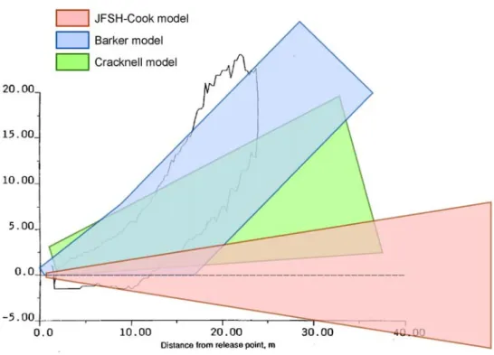
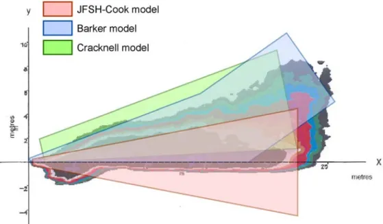
Figure 12 and Figure 13 show that the selected crude oil jet are less buoyant than the LPG jets presented in the previous subsection. In test 1 (Figure 12) the flame has lifted roughly 4 meters at a downwind distance of 25 m. In test 2 (Figure 13), the jet flame remained horizontal. A possible explanation is that a large part of the crude oil remains liquid, thereby increasing the density of the jet and reducing the buoyancy. The evaporation of droplets also reduces the temperature of the jet and thereby buoyancy.
Considering flame length, the selected models seem to underpredict for test 1 and overpredict for test 2. On the average, the JFSH-Cook model and the Cracknell model are in the right order of magnitude, while the flame length from the Barker model is slightly higher than the measured value. The total flame surface area is overestimated by both Shell models for test 2.
Considering flame lift-off, no pronounced conclusions can be drawn from test 1. The flames from the Barker and Cracknell models seem to cover the measured flame better, but the JFSH-Cook model is more aligned with the core of the flame (high occurrence percentage). For test 2, the two Shell models calculated substantial lift-off whereas the real flame remains
horizontal. The JFSH-Cook model produces a good resemblance of the flame for this test.
The fraction of heat radiated (average for test 1 and test 2) is 0.48 according to the JFSH-Cook model, 0.37 according to the Barker model and 0.39
according to the Cracknell model. The average fraction of heat radiated for the pure crude oil releases in BFETS - phase 2 was 0.40 (personal correspondence with GL Noble Denton).
Figure 12 Measured flame shape for BFETS-2 test 1 compared to model outcomes (the zone between blue and red refers to 50% flame occurrence).
Flame occurrence diagram taken from [12].
Figure 13 Measured flame shape for BFETS-2 test 2 compared to model outcomes (the orange/yellow zone between blue and red refers to 50% flame occurrence).
Table 6 Model outcomes for BFETS-2 test 1 and test 2. Measured outcome JFSH-Cook model Barker model (2) Cracknell model BFETS-2 test 1
Substance used in calculations not applicable n-nonane butane crude mix (3)
Mass involved in jet (kg/s) 5.00 5.00 5.00 Expanded jet velocity (m/s) not reported 75 81 82 Flame length (m) (1) 26 (4) 22.5 24.1 20.9
Flame width at tip (m) not reported 9.0 7.0 8.4 Flame lift off angle (°) not reported 0 35 12 Surface emiss. power (kW/m2) 287 (5) 258 255 178
Fraction of heat radiated not reported 0.46 0.37 0.33 Distance to 35 kW/m2 (m) not reported 33 28 25
Distance to 9.8 kW/m2 (m) not reported 42 39 35
BFETS-2 test 2
Substance used in calculations not applicable n-nonane butane crude mix (3)
Mass involved in jet (kg/s) 3.3 (6) 5.00 5.00
Expanded jet velocity (m/s) not reported 46 46 46 Flame length (m) (1) 23 (4) 21,2 24.1 21.1
Flame width at tip (m) not reported 8.9 7.0 11.1 Flame lift off angle (°) not reported 0 39 12 Surface emiss. power (kW/m2) 203 (5) 187 255 176
Fraction of heat radiated not reported 0.49 0.37 0.44 Distance to 35 kW/m2 (m) not reported 29 23 27
Distance to 9.8 kW/m2 (m) not reported 38 36 39
(1) The reported lengths are measured along the flame direction. The flame direction
may deviate from the release and wind directions.
(2) As discussed in the plain text, the Barker model is not designed for modelling
crude oil jet fires. It is added solely for reasons of comparison.
(3) The mix of paraffins used contained 2 mol% n-hexane, 3% n-heptane, 5%
n-octane, 5% n-nonane and 85% n-decane.
(4) According to [12] and [13], the reported flame length corresponds to the
time-averaged horizontal length of the visible flame. The reported flame lengths are a little larger than the furthest distances from the orifice to the 20% occurrence contours in Figure 12 and Figure 13. According to personal correspondence with Advantica (formerly British Gas Research), the discrepancy is caused by parts of the burning flame near the tail that are obscured by soot most of the time, and therefore are not visible in the 20% occurrence diagram.
(5) The maximum surface emissive power at any location within the visible flame as
reported in [12] and [13]. This value is fundamentally different from the average surface emissive power calculated by the jet fire models.
(6) The mass involved in the jet fire (3.3 kg/s) is smaller than the release rate
(5.0 kg/s) because SAFETI-NL predicts a considerable rainout for this scenario (78.2%). See also section 2.2.1.
3.3.3 Model outcomes for the selected butane release from JIVE
Figure 14 shows the results for the butane releases of the JIVE project ([14]). Table 7 gives the corresponding numerical data.
The butane jet fire clearly shows buoyant behaviour. The centre of the tail is about 6 m higher than the orifice position. The Cracknell model shows a very good match for the flame lift-off. The Barker model overestimates the buoyancy, while the JFSH-Cook model does not include buoyancy.
Flame length and total flame surface area are overpredicted by all three models. JFSH-Cook performs worst, with an estimated flame length of 36 m (twice as much as the real flame length). The Barker model overestimates the flame length by nearly 50%, the Cracknell model 30%.
The fraction of heat radiated is 0.50 according to the JFSH-Cook model, 0.36 according to the Barker model and 0.54 according to the Cracknell model. Unfortunately, the total amount of heat radiated is not reported in the data report.
Figure 14 Measured flame shape for JIVE test 8051 compared to model outcomes (the red line marks 40% flame occurrence, light blue 60% flame occurrence).
Table 7 Model outcomes for JIVE test 8051. Measured outcome JFSH-Cook model Barker model Cracknell model JIVE test 8051
Substance used in calculations not applicable n-butane butane butane Mass involved in jet (kg/s) 6.86 6.86 6.86 Expanded jet velocity (m/s) not reported 9.3 15 28 Flame length (m) (1) 18.3 m (2) 32.8 27.4 23.4
Flame width at tip (m) not reported 10.27 4.8 16.8 Flame lift off angle (°) not reported 0 57 23 Surface emiss. power (kW/m2) (3) 240 255 175
Fraction of heat radiated not reported 0.48 0.36 0.54 Distance to 35 kW/m2 (m) not reported 44 16.7 30.2
Distance to 9.8 kW/m2 (m) not reported 56 36.1 48.5
(1) The reported lengths are measured along the flame direction. The flame direction
may deviate from the release and wind directions.
(2) Distance from the orifice to the 20% flame occurrence tail at 6 m height, derived
from Figure 20 in [15]. The maximum horizontal distance to 50% flame occurrence is roughly 16.6 m.
(3) Only the spot surface emissive power for two locations is reported in [15]. It was
not deemed appropriate to compare spot surface emissive powers with average surface emissive powers.
3.4 Discussion of outcomes
In the previous section, outcomes of five experimental releases were
compared to predictions from the JFSH-Cook model, the Barker model and the Cracknell model. In the current section the main findings are summarised and compared to additional information found in the literature. Flame size, flame shape and flame orientation (direction) are discussed first and subsequently the amount of heat radiated by the flame will be analysed.
It is noted that the jet fire models are designed to be ‘cautiously realistic’. In order not to underestimate consequence distances along the flame direction, the flame length is calculated slightly conservative. The total amount of heat radiated is predicted as accurate as possible. As a result, the flame surface emissive power may sometimes be underestimated. A good reason to apply some conservatism in the calculation of flame length is that the radiant flame is usually bigger than the visible flame (see Figure 15). A large amount of black smoke is often seen towards the tail of the flame, which obscures the burning flame and is sufficiently warm to emit heat radiation.
![Figure 14 shows the results for the butane releases of the JIVE project ([14]).](https://thumb-eu.123doks.com/thumbv2/5doknet/3096010.9913/38.892.173.705.580.914/figure-shows-results-butane-releases-jive-project.webp)