Relative price increase for nature and ecosystem services

(1)

RELATIVE PRICE INCREASE

FOR NATURE AND

ECOSYSTEM SERVICES

IN COST-BENEFIT ANALYSIS

Background study

(2)

Relative price increase for nature and ecosystem services in cost-benefit analysis©

PBL Netherlands Environmental Assessment Agency The Hague, 2018

PBL publication number: 3214

Corresponding author

gusta.renes@pbl.nl

Author(s)

Mark J. Koetse1,2_{, Gusta Renes}1_{, Arjan Ruijs}1_{, Aart J. de Zeeuw}3

1_{PBL Netherlands Environmental Assessment Agency;}2_{Institute for Environmental Studies, Vrije}

Universiteit Amsterdam; 3_{Tilburg School of Economics and Management, Tilburg University} Acknowledgements

We are grateful to Corjan Brink, Peter van Puijenbroek, Petra van Egmond, Arjen van Hinsberg, Ron Franken, Gert Jan van den Born, Mark van Oorschot, Winand Smeets (PBL Netherlands Environmental Assessment Agency) and Bart de Knegt (Wageningen University) for their participation in, and contributions to two workshops on the relationship between ecosystems and ecosystem services. Thanks also go out to Casper van Ewijk (Tilburg University), Carl Koopmans (seo amsterdam economics, Vrije Universiteit Amsterdam), George Gelauff (Ministry of Infrastructure and the Environment), Rob Aalbers (CPB Netherlands Bureau for Economic Policy Analysis), Joop van Bodegraven and Marcel Klok (Ministry of Economic Affairs), and André Wooning (RWS – infrastructure facilities) for their advice on a draft version of the report.

Graphics

PBL Beeldredactie

Production coordination

PBL Publishers

This publication can be downloaded from: www.pbl.nl/en. Parts of this publication may be reproduced, providing the source is stated, in the form: Koets MJ, Renes G, Ruijs A and De Zeeuw AJ. (2017). Relative price increase for nature and ecosystem services in cost-benefit analysis. PBL Netherlands Environmental Assessment Agency, The Hague.

PBL Netherlands Environmental Assessment Agency is the national institute for strategic policy analysis in the fields of the environment, nature and spatial planning. We contribute to

(3)

Abstract

In 2015, the Dutch working group on discount rates (Werkgroep Actualisatie Discontovoet) recommended using the standard discount rate in cost-benefit analyses (CBAs) of nature, while taking into account annual relative price increases of 1% for the effects on ecosystem services. The increase is not to be applied if the particular ecosystem service is substitutable. In this report, we examine for which ecosystem services CBA researchers need to apply the 1% increase. At issue is the change in the ecosystem services that directly affect people’s welfare, known as final ecosystem services, such as food supply, drinking water, flood protection, quality of the environment, green recreation and natural heritage. Changes in intermediate services, such as pollination and carbon sequestration, have an indirect impact on welfare, through their effects on final services and conventional consumption.

Two matters play an important role in determining the relative price increase: the relative growth rate of nature compared to the growth rate of consumption, and the degree to which nature is substitutable. If nature grows more slowly than consumption and is not or only partly substitutable, it will become scarcer in the future. This justifies the application of a relative price increase. The data show that, over the past few decades, ecosystem services have become comparatively scarcer in the Netherlands: the annual growth rate of GDP was between 0 and 3% higher than that of ecosystem services. However, data published in international studies reveal that the elasticity of substitution between ecosystem services and conventional consumption is generally greater than 1. Therefore, substitution of

ecosystem services with other goods or services is, to a certain extent, possible. Combining both insights, it appears that on the basis of historical data a relative price increase of 1% is defensible for a large share of ecosystem services, even though they are all substitutable to some degree. A look at the latest WLO scenarios (CPB/PBL, 2015a) about future growth rates of nature and consumption provides comparable results.

When highly location-dependent ecosystem services become comparatively scarce in or near urban areas, their marginal utility increases, which means that a relative price increase of more than 1% can be justified. Several provisioning services, such as those related to food, wood and energy, should not be subject to relative price increases, because technology-based substitutions or imported goods ensure that the growth in their supply keeps pace with the growth in consumption. In contrast, a worldwide decline in provisioning services could give rise to the application of a relative price increase.

(5)

1.Introduction

1.1 Background and definition of the problem

A CBA appraises an intervention’s positive and negative effects on welfare, that is to say, the measure’s costs and benefits for society. The benefits and the costs are often spread out over time. Ideally, future developments in prices and values are used to calculate future costs and benefits, so that differences in the relative scarcity of goods and services are taken into account in a CBA and in policy decisions based on the analysis. In a CBA, relative prices are often assumed to remain stable over time (i.e. the discount rates for several goods and services are assumed to be equal to each other), and as a result, future

variations in relative scarcity are not reflected. The assumption is made because estimating future prices is a complicated task. This applies not only to conventional consumption, but especially to estimates of prices or values of goods and services for which no market exists. Particularly with regard to public goods and services which are becoming comparatively scarce, such as nature and the ecosystem services it provides, the assumption that relative prices remain stable, proves to be problematic because these prices may not be assigned enough weight in the CBA (the CBA balance) nor, consequently, in the decision-making process.

For this reason, the following recommendation was included in the report by the working group on discount rates (Werkgroep Actualisatie Discontovoet, 2015: p. 6), and adopted by the Dutch Government (see Ministerie van Financiën, 2015):

For the discounting of nature (operationalised, for example, as ecosystem services, biodiversity and landscape), the working group recommends using the standard discount rate, while allowing for an annual 1% price increase for nature. This results in an effective discount rate of 2%. Nevertheless, nature should be discounted at the standard rate and without applying price rises, if it can be demonstrated that the features of nature in question are substitutable.

As of yet, there is hardly any scientific literature that supports the application of relative price increases for nature in CBAs. On the basis of their recent empirical study, Baumgärtner et al. (2015) promote the idea that there are good reasons for applying a relative price increase for nature and ecosystem services. The recommendation of the 1% price increase put forward by the Dutch working group on discount rates is partly based on this article. There are two factors underlying this result. First, the growth rate of ecosystem services is lower than that of conventional consumption (which in that study is measured by means of GDP). Second, ecosystem services and conventional consumption are not (perfect)

substitutes. Both observations are derived from global data and scientific literature on ecosystem services.

For researchers who are drawing up CBAs that involve nature effects or are aimed at supporting nature policies, this report provides a preliminary recommendation, stating how to determine whether they need to apply a relative price increase of 1%, and if so, which changes in nature or ecosystem services are subject to the increase. To support this advice, it is particularly important to verify if the empirical evidence collected by Baumgärtner et al. also applies to the Netherlands. To do this, we look at two aspects. First, we check whether in the Netherlands too, the growth rate of ecosystem services is lower than the growth rate of conventional consumption. Second, we research and argue the extent to which ecosystem services and conventional consumption are substitutable, and how this varies for each

(6)

ecosystem service. In the next section we discuss the applied conceptual framework, and describe the structure of the rest of this report.

1.2 Conceptual framework

A CBA produces an estimate of the welfare effects of an intervention. Before discussing which theoretical considerations are to form the basis for determining whether a relative price increase or a lower discount rate should be applied to nature in CBAs, this section first present a conceptual framework that describes how nature affects welfare. In this

framework, we make a distinction between the biophysical system and the economic system (see Figure 1).

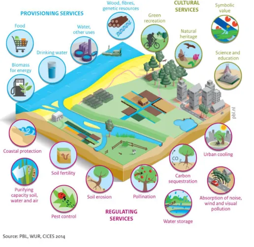
The biophysical system describes nature as a collection of different ecosystems, such as forests, heathlands, grasslands and lakes. Interventions assessed by a CBA can affect both the spatial extent and the quality of ecosystems. These ecosystems provide humans with all kinds of goods and services, often referred to in short as ecosystem services. The CICES-system distinguishes the following groups (see also Figure 2 and De Knegt et al., 2014): • provisioning services, such as food, fish, biomass, drinking water and genetic resources; • regulating services, such as soil fertility, water regulation, pollination, natural pest

suppression and carbon sequestration;

• cultural services, such as green recreation, natural heritage and the symbolic value of nature.

The quality, or health, of an ecosystem is also measured by means of the biodiversity within it. A high degree, or a certain degree, of biodiversity is particularly important for the

provision of ecosystem services in the future.

Figure 1. Conceptual framework, distinguishing between intermediate ecosystem services and final ecosystem services, and between substitution in welfare functions and substitution in production functions1

For CBAs, it is important to gain insight into the changes in ecosystem services that lead directly to a change in their utility for humans, that is, a change in human welfare. To do so,

(7)

we make a distinction between intermediate ecosystem services and final ecosystem services. Human welfare is directly affected by changes in final services, such as the provision of food, drinking water, flood protection, environmental quality (e.g. air quality and protection against hot weather), green recreation, nature’s symbolic value and natural heritage.2_{Changes in intermediate services, such as soil fertility, pollination and carbon} sequestration, indirectly lead to changes in welfare as they affect the supply of both conventional consumption and final services.3_{Conventional consumption and final services} are provided through production functions, which also use capital, labour and technology as input factors, in addition to intermediate ecosystem services (see Figure 1).4_Substitution between these input factors is, to a certain extent, possible. This concerns substitution

between factors in the production function of final services. Examples include the

substitution of natural pest control with the application of pesticides or the substitution of the soil’s water purifying capacity by water treatment plants.

Figure 2. Overview of the various types of ecosystem services in the CICES system

2 _{The CICES classification of ecosystem services categorises the symbolic value of nature and natural heritage} as cultural ecosystem services. This is a case of non-material ecosystem output that affects people’s physical and mental condition (de Knegt et al., 2014). In the Netherlands, symbolic value is mainly related to the importance that people attach to the preservation of emblematic plant and animal species, such as the white-tailed eagle, the stork, the grouse, the goose, the seal, the fox, the wolf, the viper and the large copper. The value of natural heritage has to do with the willingness to pay for nature to be preserved as a legacy for future generations. Examples of this are the preservation of rare species on the Red List (list of endangered species) and of target nature types as defined in the Birds and Habitats Directives.

3_{The distinction between intermediate and final services is meant to avoid double counting in the CBA. For} example, double counting occurs when both the decline in soil fertility and the decline in agricultural production are measured, or when the increase in carbon sequestration is measured along with the decrease in the impact of climate change.

4_{In the report by the working group on discount rates, technology is identified as a factor that can affect the} demand for certain goods and services, in reference to both conventional consumption and consumption of ecosystem services. The report also states that technological development in particular is difficult to predict. This is very much comparable to the role played by technology as input in production functions, as illustrated in Figure 1.

(8)

In our framework, welfare in the economic system is determined by conventional

consumption and consumption of final ecosystem services. They both are input factors in the welfare function, and combined, they ultimately produce welfare. This also means that they may be substitutes for each other. That is to say that, theoretically, a decline in welfare due to a decrease in the provision of final ecosystem services can be partly offset by an increase in conventional consumption. Examples of this are substituting a walk in a forest for a visit to an amusement park and replacing tap water with imported bottled water. The point at issue is substitution among the components of the welfare function. This form of substitution is also the central feature in the underlying scientific literature on discount rate

differentiation. The report by the working group on discount rates (Werkgroup Actualisatie

Discontovoet, 2015) uses substitution in a broader sense, and assigns an important role to

substitution in the production functions. Substitution between intermediate ecosystem services and technological input factors in the production functions is also important for the question of whether a different discount rate may be used for changes in nature, and is relevant for measuring the effects on final services when carrying out a CBA. In this report we make a clear-cut distinction between the two forms of substitution. Firstly, because they affect the discount rate in two different ways, and secondly, because the distinction is important to avoid misunderstandings arising between ecologists and economists.

1.3 Report structure

The rest of this report is structured as follows. In Chapter 2, we start with a discussion of the theoretical framework. Conform the better part of the international literature on discount rates, we use the Ramsey growth model (1928) and the pertinent Ramsey rule. This rule states that two aspects determine whether a relative price increase for ecosystem services is justifiable.

Firstly, we need to compare the historical growth rate of ecosystem services to that of conventional consumption. The intuitive understanding is that, if ecosystem services become relatively scarcer, they will also become relatively more valuable. The analysis of the growth rates of ecosystem services and consumption is carried out in Chapter 3. It reveals, among other things, that there is only a limited amount of historical data on final ecosystem services, which means we have to resort to historical data on nature and intermediate services as indicators.

Secondly, we need to assess the degree to which final ecosystem services and conventional consumption can substitute each other in the welfare function. After all, if a decrease in utility caused by the relative scarcity of ecosystem services can be fully offset by a rise in conventional consumption (i.e. perfect substitution), then that relative scarcity will not produce an increase in the relative price, and therefore CBAs of ecosystem services have no basis for the application of a relative price increase. This leads to the examination in

Chapter 4 of the extent to which ecosystem services and conventional consumption are

substitutable.

In Chapter 5 we investigate the range for the relative price increase, using the Ramsey rule described in Chapter 2, the relative growth rates from Chapter 3 and the information on options for substitution from Chapter 4. A key assumption in this step is that the

relationship between intermediate ecosystem services and final ecosystem services is linear. The assumption is necessary because we only have growth rates for intermediate services at

(9)

In Chapter 6 we expand our framework and discuss the role of production functions of final ecosystem services and the role of substitution between, on the one hand, nature and intermediate ecosystem services, and on the other hand, technology. This chapter serves two purposes. First of all, we look into the potential consequences of deviations from the assumption made in the previous chapter, i.e. an examination of the effects that non-linear production functions have on the discount rate. Secondly, we investigate the degree to which the existence of tipping points in production functions can be a reason for using data on the ecological system itself and for applying precautionary principles in the CBA.

The key findings from our analyses in Chapters 2 to 6 are presented in Chapter 7, which also puts forward our recommendations on the use of relative price increases for ecosystem services. Chapter 8 rounds off the report with conclusions and a discussion, and a

deliberation on the lines of follow-up research on ecosystems and ecosystem services that are critical for gaining broader and deeper insights into the relative price of nature and ecosystem services.

(10)

2.Theoretical

framework and the

Ramsey rule

Ideally, a CBA contains costs and benefits for the present and the future, expressed in monetary terms. This means that, among other things, both the current and future monetary value of ecosystem services needs to be measured. Considerable progress has been made in the area of valuing goods and services that are not traded on markets (known as non-market valuation; for an overview of valuation practices, see Koetse et al., 2015, and several other publications). However, at present, it is difficult to establish the monetary value for many ecosystem services, let alone to make meaningful statements about future

preferences and prices on the basis of present-day valuation studies.

This report uses a theoretical framework to gain insight into future relative prices, without the need for measuring them explicitly. The model is based on the fundamental economic idea that the price of a good increases when it becomes scarcer, and by extension, that in the case of imperfect substitution, the relative price of a good increases when it becomes

relatively scarcer. This model is also used in Baumgärtner et al. (2015), and takes the form

of an extended version of the Ramsey growth model (1928), which uses a utility function5 applicable to a representative consumer and makes a distinction between conventional consumption (C) and consumption of ecosystem services (E), where both C and E are exogenous. The model only considers those ecosystem services that can be categorised as

final ecosystem services, i.e. those services which benefit humans in a direct manner. This is

in line with CBA practice in the Netherlands, where only final services may be factored in to avoid double counting of welfare effects. The welfare function used by Baumgärtner et al. (2015) is as follows:





0

,

t t t t

W

U C E e

dt

  





. (1)

Here, ρ represents the growth rate of pure time preference. The standard Ramsey rule for the welfare function in (1) does not consider ecosystem services separately and is given by:

 

'

t t

d

U C

dt

r

U C



  

. (2)

The marginal productivity of capital, interest rate r, must be equal to time preference rate ρ minus the growth rate of marginal utility U’(C). Conversely, therefore, the interest rate is the same as the discount rate. As consumption increases, the marginal value falls and the discount rate rises. For a standard CRRA (constant relative risk aversion) utility function

U(C) = C1-γ_{/(1-γ) the Ramsey rule acquires its well-known form:}

 

''

'

t t t t t

C U

C

r

g

U C

C



  

   

, (3)

(11)

does increase, it is necessary to apply a lower discount rate for ecosystem services. The

Ramsey rule (2 and 3) can easily be extended to separate the discount rates for

conventional consumption and the consumption of ecosystem services, based on the welfare function (1). This gives the formulas (see Weikard and Zhu, 2005):

,

C CC C CE E E EC C EE E

r

g

r

g

   

 

   

 

, (4)

where rC and rE are the discount rates for consumption and ecosystem services,

respectively, gC and gE are the corresponding growth rates, and the four elasticity values are

CC = -CUCC/UC, CE = -EUCE/UC, EC = -CUEC/UE and EE = -EUEE/UE.

The difference between discount rates rC and rE can be expressed in the growth rate of the

relative price of ecosystem services compared to consumption, P, which is given by:



/



/

E C P E C

d

U

P

_dt

g

P

U



. (5)

Using (4) to work out (5) gives the simple equation rC – rE = gP (see Weikard and Zhu,

2005, and other publications). This means that the difference between discount rates rC and

rE is, in simple terms, equal to the growth rate of the relative price of ecosystem services

compared to consumption. In actual practice, it is then possible to use a fixed discount rate

rC, while making adjustments to the discount rate for ecosystem services rE by conducting

research into developments in relative prices.

It is also important to include the possibilities for substitution of ecosystem services in the derivations. A further specification of the utility function U(C,E) as a CES utility function with a constant elasticity of substitution σ (Hoel and Sterner, 2007) implies that the growth rate of the relative price, and therefore the difference between the discount rates, can be expressed as:





1

C E P C E

r



r



g



g



g



. (6)

This means that the difference between the discount rates of (in the case at hand) ecosystem services and consumption is related to the difference in growth rates and the

degree of substitution between the two variables. The underlying idea here is that future

relative scarcity of a good or service (lower growth rate) will lead to an increase in the relative price ─ that is, a lower discount rate. It is important to note that setting a difference between discount rates in a CBA is equivalent to applying a relative price increase which equals the difference between the two discount rates. In other words, a 1% decrease in the discount rate for ecosystem services is the same as a 1% increase in their relative price. The formula also shows that the two discount rates are the same if there is perfect

substitution (σ → +∞), or if the growth rates are equal (gC = gE).6 This also shows that two

essential elements are involved in determining relative price: the difference between the growth rates of final ecosystem services and of consumption (relative scarcity), and the potential for substitution.

When an ecosystem service, or the potential for delivery of the service, grows more slowly than consumption or is on a downward trend, then that may be reason to apply a relative price increase. As shown in Baumgärtner et al. (2015), there is quite a bit of variation in these growth rates, both within countries and for the world as a whole. However, the average growth rate of ecosystem services was significantly lower than that of consumption

6_{The use of a CES utility function means that the applicable discount rate itself is not constant over time. Since} this report deals mainly with the relative discount rate, we are not taking this complicating factor into account at this stage.

(12)

in the period covered by their study. The fact that something becomes relatively scarcer does not automatically imply that a relative price increase must be applied. For if the ecosystem service in question is to a large degree substitutable with conventional consumption, the relative growth rate is less important. Therefore, to approve the

application of a relative price increase, it must be demonstrated that the ecosystem service is not substitutable with conventional consumption. However, the degree of substitutability between goods and services lies on a continuum from zero (goods are perfect complements) to infinite (goods are perfect substitutes). It is therefore, as will become apparent later, almost impossible to prove that an ecosystem service is not substitutable with conventional consumption, because a certain degree of substitution is always conceivable. Therefore, when deciding whether to establish a relative price increase for ecosystem services, it is far more important to consider the relative growth rate of ecosystem services compared to consumption and the degree to which ecosystem services can be substituted with consumption.

Finally, we need to restate that a CBA should, in principle, measure changes in final ecosystem services, but that intermediate services, regulating services in particular, are needed for the production of final services. A drop in the provision of intermediate services may lead to a decrease in the capacity to provide final services in the short or long term. As long as a decrease in intermediate services can be translated into a decrease in final

services, this is not an issue, since the reduction in final services can be included in a CBA. However, as the next chapter shows, there are only very limited data on final ecosystem services and their evolution. For this study, data on nature itself or data on intermediate services can be used as indicators for trends in final services, whereby an assumption must be made about the relationships between nature and intermediate services on the one hand, and final services on the other. This is discussed in more detail in the following chapters.

(13)

3.Growth rates of

ecosystem services

and conventional

consumption in the

Netherlands

Data on the historical development of final ecosystem services in the Netherlands are very limited. An exception to this is the data collected on, mainly, provisioning services.7_Some final services, such as green recreation, quality of the environment, symbolic value of nature and natural heritage, have not been unambiguously defined yet. Consequently, not much is known about final services, not to mention the fact that the long data series needed to calculate growth rates are unavailable. However, we do know that the provision of final services depends on a number of indicators for ecosystem quality and ecosystem quantity. These elements are necessary for the provision of final services and therefore they can be used as indicators for changes there. For these indicators, longer data series do exist.

Accordingly, the analysis presented in this chapter does not provide a hard estimate of the growth rate of final ecosystem services. Our aim is to make a plausible argument that the growth rates of conventional consumption and final services diverge, but not to indicate exactly by how much. Later, we will make assumptions about the relationship between our indicators and final ecosystem services (i.e. the production function), but at this point we limit ourselves to measuring the growth rates of the indicators for ecosystem quality and ecosystem quantity.

For the distinction between quality and quantity of ecosystems, we differentiate between data on biodiversity, as an indicator for quality, and data on land-use surface areas, as an indicator for quantity. Both offer clues about changes in green recreation, quality of the environment, symbolic value of nature and natural heritage. The growth rates are compared to the growth rate of real conventional consumption in the Netherlands, and all figures are converted to per-capita values, using the Dutch population trends from Statistics

Netherlands (CBS StatLine). The data on conventional consumption have been retrieved from the Central Economic Plan drawn up by CPB Netherlands Bureau for Economic Policy Analysis (CPB, 2017). The real household consumption and care consumption indices for the 1970–2015 period are taken from the annex to the Central Economic Plan, and a weighted average is calculated from these two series using the respective nominal volumes of household consumption and care consumption as weights. The resulting series is our indicator for real conventional consumption. The reason for refraining from using GDP, as in Baumgärtner et al. (2015), is that consumption is part of the Ramsey rule rather than GDP.

7_{Note that the historical data on agricultural production provide little insight into the provision of intermediate} ecosystem services or the quality of the ecosystem because a large part of the increase in agricultural efficiency is the result of technological input factors.

(14)

The growth rates of consumption and GDP are not equal. This is shown in Figure 3, which contains the indices of real GDP and three real consumption series, for the 1970–2015 period. It shows that household consumption grew less than GDP and that the increase in the consumption of care services was substantial. As a result, total consumption grew slightly less than GDP. The growth rate for GDP per capita over the whole period was 1.66%, while the growth rate for total consumption was 1.40%, a difference of about a quarter of a percentage point.

3.1 Indicators for ecosystem quality: biodiversity in the

Netherlands

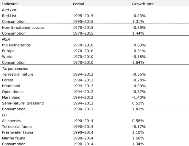
To gain insight into changes in the quality of our ecosystem, we need historical data on the indicators that are used in environmental impact assessments. However, since these data are not available, we use data on developments in biodiversity. These are obtained from the website of CLO (Environmental Data Compendium) and measure plant and animal species that are, and those that are not on the Red List, mean species abundance (MSA), target species, and the living planet index (LPI). Combined, they tell us something about trends in biodiversity in the Netherlands and they also give an indication of changes, particularly those affecting the symbolic value of nature. Figure 4 shows the indices of these data sets, which are the basis for the calculation of yearly growth rates. In contrast to the growth rate of conventional consumption, these series and growth rates are not calculated per capita, as they are non-rival ecosystem services. The growth rates of ecosystem quality are presented in Table 1, along with the growth rate of per-capita conventional consumption for the same periods. Virtually all indices are found to have a flat or a slightly declining trend, while consumption over the studied periods has grown steadily. The result is that biodiversity (as an indicator for ecosystem quality) is becoming relatively scarcer in relation to conventional consumption.

(15)

Note: Top left: threatened and non-threatened species; top right: mean species abundance (MSA) in the

Netherlands, Europe and worldwide; bottom left: target species for several ecosystems; bottom right: living planet index (LPI) for several ecosystems)

(16)

Table 1. Growth rates of indicators for biodiversity (not per capita) in relation to growth rate of conventional consumption per capita

Indicator Period Growth rate

Red List Red List 1995–2015 -0.03% Consumption 1995–2015 1.31% Non-threatened species 1970–2015 -0.65% Consumption 1970–2015 1.44% MSA the Netherlands 1970–2010 -0.89% Europe 1970–2010 -0.31% World 1970–2010 -0.18% Consumption 1970–2010 1.64% Target species Terrestrial nature 1994–2012 -0.56% Forest 1994–2012 -0.28% Heathland 1994–2012 -0.90% Open dunes 1994–2012 -0.37% Marshland 1994–2012 -1.40% Semi-natural grassland 1994–2012 0.53% Consumption 1994–2012 1.42% LPI All species 1990–2014 0.58% Terrestrial fauna 1990–2014 -0.17% Freshwater fauna 1990–2014 1.10% Marine fauna 1990–2014 1.60% Consumption 1990–2014 1.34%

3.2 Indicators for ecosystem quantity: surface area of nature

in the Netherlands

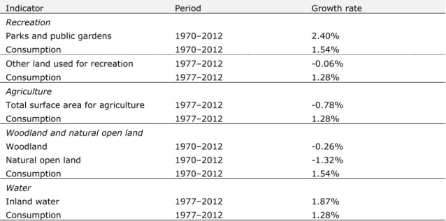
The provision of ecosystem services is directly related to the surface areas of the different kinds of ecosystems from which they originate. Data on areas for various types of land use are obtained from the StatLine database from Statistics Netherlands. We have retrieved data on the surface areas of recreation sites, agriculture, forests and open natural land, and surface waters. The per-capita indices of these data series, presented below in Figure 5, show slightly upward or stable trends in the case of recreation sites and surface water, but for forests, open natural land and agriculture the surface areas are steadily decreasing. Table 2 shows the per-capita growth rates of these surface areas compared to per-capita conventional consumption in the same time periods. From this it is clear that the growth rate of the surface area dedicated to parks and public gardens is higher than that of consumption. The same applies to the growth rate of the total area of surface waters. The growth rates of other surface areas — other kinds of recreation sites, agriculture and forests and open natural land — are considerably lower than the growth rate of consumption.

(17)

(18)

Table 2. Per-capita growth rates of land-use surface areas compared to growth rate of conventional consumption per capita

Indicator Period Growth rate

Recreation

Parks and public gardens 1970–2012 2.40%

Consumption 1970–2012 1.54%

Other land used for recreation 1977–2012 -0.06%

Agriculture

Total surface area for agriculture 1977–2012 -0.78%

Woodland and natural open land

Woodland 1970–2012 -0.26%

Natural open land 1970–2012 -1.32%

Water

Inland water 1977–2012 1.87%

3.3 Regional developments

In addition to studying developments for the Netherlands as a whole, it is also interesting to consider developments in several regions within the country, in order to draw conclusions about regional differences in the relative scarcity of ecosystem services. This may be

relevant to those ecosystem services that are provided locally. Examples are cultural services (including green recreation and the aesthetic value of the living environment) and regulating services (including air quality and water quality). For the twelve provinces, data compiled by Statistics Netherlands (CBS) are available on the surface areas of land use for the period 1987–2011. Unfortunately, no realistic figures are available for conventional consumption at the provincial level, and therefore we use GDP as an indicator for consumption. The resulting regional differences will only be distorted if the difference in growth between consumption and GDP varies (greatly) among provinces; for example, if in North Holland consumption grows less rapidly than GDP, while both grow at the same pace in Gelderland. The figures for province-level nominal GDP for the period 1988–2015 have been obtained from Statistics Netherlands. They have been converted to real GDP in 1988 prices and adjusted for GDP price changes for the Netherlands using figures from the Central Economic Plan drawn up by CPB (CPB, 2017). Since population trends also vary among provinces, the figures for GDP and surface areas of land use are expressed per capita. To achieve this, the study uses data from Statistics Netherlands on population trends in each province for the period 1988–2015. Table 3 presents the growth rates of real GDP per capita and of surface area of forms of land use per capita for the 12 provinces over the period 1988–2012.

Considerable differences exist among provinces in terms of both income and trends in surface areas of land uses and these could in theory also lead to differences in the relative prices for consumption (expressed by means of GDP in this part of the study) and ecosystem services. It is interesting to look at differences between the provinces in Randstad (a

conurbation in the western part of the country, covering large parts of North Holland, South Holland and Utrecht) and the other provinces. Table 4 presents the average growth rates for different types of land use and real GDP for the Randstad provinces and for the other provinces. The difference between the GDP growth rates is very small, and the same applies

(19)

not becoming relatively scarcer. One conclusion that could be reached from this is that a CBA needs to give more weight to changes in those two types of land use (inland water, and parks and public gardens) in the Randstad conurbation than in other regions. In other words, changes in inland water, and parks and public gardens in the Randstad conurbation could be given a relative price increase of 1%, while in other regions they would not qualify for this kind of adjustment. It should be noted that, when measuring geographical differences in cultural services, the province is in all likelihood not the most suitable scale and it is probably more appropriate to use an additional distinction based on level of urban development. A distinction of this kind would undoubtedly also reveal significant regional and local differences.

Table 3. Per-capita growth rates of real GDP and surface area of forms of land use by province for 1988–2012

Real GDP Inland water Woodland Natural open land Parks and public gardens Agricultural land Groningen 3.04% 0.94% 2.87% 0.93% 1.80% -0.38% Friesland 1.71% 4.57% 0.49% -0.08% 2.60% -0.48% Drenthe 1.52% 1.71% 0.27% -0.11% 4.17% -0.71% Overijssel 2.09% -0.19% -0.32% -0.85% 1.97% -0.83% Flevoland 2.11% 3.63% -2.08% -3.17% 0.78% -2.80% Gelderland 2.23% 0.22% -0.19% -0.92% 1.88% -0.70% Utrecht 2.50% -1.48% -0.90% -1.31% 1.87% -1.21% N. Holland 2.45% 4.09% 0.55% -0.74% 1.86% -0.88% S. Holland 2.07% -0.18% 2.14% -0.18% 1.43% -0.96% Zeeland 1.02% 0.08% 1.76% 0.29% 2.63% -0.49% N. Brabant 2.67% 0.35% -0.19% -0.69% 2.36% -0.82% Limburg 2.03% 1.61% 0.37% -0.77% 3.78% -0.35% Table 4. Per-capita growth rates of real GDP and land use for Randstad provinces and rest of provinces in the period 1988–2012

Real GDP Inland water Woodland Natural open land Parks and public gardens Agricultural land Randstad 2.30% 1.65% 0.28% -0.58% 1.63% -0.95% Other 2.26% 3.04% -0.01% -0.47% 2.43% -0.71%

3.4 Data on ecosystem services

As mentioned above, data and information on the provision of ecosystem services in the Netherlands are limited, and important insights into the functional relationship between ecosystems and ecosystem services are still lacking. An exception to this is a report by De Knegt (2014), which, among other things, maps the provision of a range of both

intermediate ecosystem services and final services. While the list is not exhaustive, it does contain a large number of important services and draws a good picture of the diversity among them. Figure 6, taken from the report, shows that the provision of many ecosystem services in 2013 had decreased or remained stable compared to 1990.

This means that the growth rate of those services is considerably lower than that of

conventional consumption, and can be even negative. It does appear that the rates for food and energy production, water retention capacity and the symbolic value of nature increased in that period. However, it is not likely that these growth rates are equal to or higher than that for consumption, which grew by 1.92% per year on average in the period 1990–2013, but there are no data available to verify this. The Natural Capital Accounts, which are currently being developed by Statistics Netherlands within the environmental accounts system, may be able to provide additional insights into this in the future.

(20)

It is important to realise that the list in Figure 6 contains both final services and intermediate services. Although final services do, in principle, play a role in the CBA and intermediate services do not, in actual practice it is often difficult to assess measures for their effects on final services, while their effects on intermediate services and nature are evaluated more easily. This is why assessments of the relative scarcity of intermediate services and nature continue to be of relevance.

3.5 Conclusion and discussion

Data on the evolution of supply and demand in regard to ecosystem services are scarce, but the amount available does reveal that the growth rate of most ecosystem services is falling behind that of conventional consumption. It should be noted that the information is often incomplete, of a qualitative nature or based on estimates. However, data on the underlying ecosystems and nature also show that, in the vast majority of cases, these are becoming

(21)

The data on ecosystems and nature serve, of course, as indicators for the final ecosystem services which ideally we would prefer to measure directly. After all, the question we are addressing is not whether biodiversity is becoming relatively scarcer, but rather, whether such scarcity means that the provided final ecosystem services are becoming relatively scarcer. This highlights the need to collect more data and information on the evolution of ecosystem services, and the need to acquire knowledge about their characteristics, quality and production functions, and the role of ecosystems in these functions (see also Chapter 6). At this stage, we assume that there is a linear relationship between the indicators we use and the final ecosystem services. Under this assumption, our results show that the growth rate of consumption is higher than that of ecosystem services, and that therefore ecosystem services have become relatively scarcer in recent decades. In quantitative terms, the

(22)

4.Substitution between

ecosystem services

and consumption in

the utility function

To determine the relative price increase of ecosystem services, it is important to have a clear picture of not just the relative growth rate of the services, but also the possibilities of

replacing or substituting them with conventional consumption. For our purposes, it is therefore relevant to gain insight into the possibilities for substitution between ecosystem services and consumption in the welfare function. The core concept here is elasticity of

substitution (see Equation 6). In virtually all analyses on this subject, a CES function is used,

which is characterised mainly by a constant elasticity of substitution between — in our case — consumption (C) and ecosystem services (E). Ebert (2003:452–453) shows that in a CES utility function, the elasticity of substitution σ between E and C is derived from the income elasticity of willingness to pay (WTP) for E.This is equal to 1/σ and measures the percentage change in WTP for E which results from a 1% increase in income. The literature contains many estimates of this elasticity. Baumgärtner et al. (2015) use an estimate derived from a meta-analysis of contingent valuation studies on WTP for biodiversity (Jacobsen and Hanley, 2009). This meta-analysis uses 145 different estimates of WTP for biodiversity, taken from 46 contingent valuation studies. The analyses in this study give an average income elasticity of 0.38, which means that an income increase of 1% causes WTP for biodiversity to rise by 0.38%. This corresponds to an elasticity of substitution of approximately 2.6. It appears that biodiversity and conventional consumption are to some extent substitutable.

This result is in agreement with other findings in the literature. An overview of parameters in Drupp (2016) shows that values of the elasticity of substitution reported in the scientific literature are, almost without exception, higher than 1, with many even well above 1 (see Table 5). The work also shows that this applies to a wide variety of services, including biodiversity, woodland services, wetland services, air quality, water quality, landscape amenities and recreation (for other recent publications see Brander and Koetse, 2011). Studies specific to the Netherlands are scarce. Bouma and Koetse (2017) have conducted a contingent valuation study of Dutch citizens’ willingness to pay for extensive agriculture which brings substantial biodiversity benefits. The authors have found a positive correlation between income and WTP for biodiversity, with a corresponding elasticity of substitution between 1.7 and 2, depending on the chosen model specification.

(23)

Table 5. Estimates found in the literature of elasticity of substitution between ecosystem services and conventional consumption

Study Ecosystem service Elasticity of

substitution σ Martini and Tiezzi (2014) Air quality improvement 0.86

Schläpfer and Hanley (2003) Landscape amenities 1.11

Lindhjem and Tuan (2012) Biodiversity 1.37

Hökby and Söderqvist (2003) Collective ecosystem services 1.47 Ready et al. (2002) Water quality improvement 1.69 Liu and Stern (2008) Collective marine ecosystem services 2.38

Jacobsen and Hanley (2009) Biodiversity 2.63

Broberg (2010) Contingent value of predator species 2.70 Carlsson and Johansson-Stenman (2000) Air quality improvement 3.13 Chiabai et al. (2011) Collective woodland ecosystem

services

3.23 Söderqvist and Scharin (2000) Water quality improvement 3.70 Wang and Whittington (2000) Air quality improvement 3.70 Barbier et al. (2015) Water quality improvement 3.85 Whitehead et al. (2000) Recreation services improvement 4.17 Hammitt et al. (2001) Preservation of wetlands 4.55 Wang et al. (2013) Water quality improvement 4.76 Yu and Abler (2010) Air quality improvement 5.00

Barton (2002) Water quality improvement 7.14

Source: Calculations based on Table 1 in Drupp (2016)

These estimates indicate, almost without exception, that the elasticity of substitution σ is greater than 1. This means that, generally speaking, conventional consumption and

ecosystem services are substitutable in the welfare function, but also that they are not perfect substitutes. The estimates also suggest that the possibilities of substitution in the welfare function differ somewhat from one ecosystem service to another.

Location-specific ecosystem services

Ecosystem services that are strongly tied to their location are a possible exception to these insights. Important examples of this are the provision and quality of outdoor recreation in the living environment, and the quality of the living environment itself (not only with regard to aesthetics but also to air quality). This might also apply, to a lesser degree, to the working environment. Particularly in areas with high levels of urban development, the provision of these services is under pressure.The central debate here is about the extent to which these services can be substituted with conventional consumption. For example, to what degree can a decline in utility, caused by a lack of supply or poor quality of recreation in the living environment, be substituted with utility obtained from additional consumption or indoor recreation (e.g. watching TV, gaming, visiting theatres and cinemas)? The answer to this question will vary per person, but many will strongly argue that these things are highly complementary, and that therefore outdoor recreation is only substitutable with consumption and indoor recreation to a limited extent.8_{However, empirical literature on this specific issue} is largely lacking, and therefore further research is desirable.9_{Until the moment such}

research reveals otherwise, it seems sensible to assume that possibilities for substitution are limited in those places where the provision of local ecosystem services is under pressure and

8_{Outdoor recreation may, to a limited extent, also be substitutable with holidays abroad.}

9_{In a theoretical study, Drupp (2016) examines the presence of what he calls subsistence levels, and the} consequences they have on a relative price increase of ecosystem services. The finding was that subsistence levels cause the relative price of ecosystem services to go up. Our considerations concerning scarcity of local-level ecosystem services share similarities with these subsistence local-levels. The argumentation is that if, for example, the local air quality falls below a certain level, this will have a significant effect on the welfare of the people living and working at that particular location. Further research is required into the existence of such tipping points in the utility function.

(24)

therefore becoming relatively scarce than GDP. This, logically, will apply particularly to highly developed urban areas.

Substitution with technology and imports

In addition to substitution with conventional consumption in the welfare function, there is also substitution of ecosystem services in the production function. Those (intermediate) ecosystem services that are a factor in production systems can be substituted with

technology. Examples include the use of fertiliser and pesticides in agriculture, and the use of digital technology to improve the quality of recreation. Some final ecosystem services, the provisioning services in particular, can also be substituted with imports. Strictly speaking, we are dealing with forms of substitution which ensure that the relative growth of final services keeps pace with conventional consumption (see Chapter 6 for details).

A report by De Knegt (2014) provides information on these two forms of substitution and, for several intermediate and final services, presents estimates of substitution with imports and with technological alternatives. An overview is provided in Figure 7. Substitution with imports is particularly relevant for provisioning ecosystem services, especially food, wood and

energy. In fact, any natural product that is traded on international markets is substitutable with foreign products. The underlying assumption is that, at the global level, provisioning services are not becoming scarcer. The facts also indicate that provisioning services have a global nature and that their growth rates are important at the international level.

Technological alternatives are available, particularly for water supply, water retention, soil fertility, coastal protection, water purification and pest control. Of these services, especially water supply and water retention can, to some degree, be labelled as final services which can be replaced (in part) by technological alternatives. This would be a case of substitution in the welfare function. The other categories are intermediate services, where technological alternatives are a case of substitution in the production function. Examples of this include fertilisers and pesticides, which are used as a substitute for natural soil fertility and natural pest control produced by ecosystems. In Chapter 6 we discuss this form of substitution in greater detail. It is important to note that technological substitution often brings about externalities, which play an important role in cost-benefit analyses. These may affect other ecosystem services, but also the very service for which the technology is the substitute. Soil productivity is, once again, a good example: while productivity can be improved by the use of fertilisers and pesticides, these technological tools produce negative effects in the longer term. These externalities should be identified and included in the cost-benefit analysis.

(25)

(26)

5.Relative price

increase for

ecosystem services

In this chapter we determine the range in which the relative price increase of ecosystem services may fall. This is based on data on growth rates and the potential for substitution, as presented above. For the growth rates we use, firstly, data on surface areas of ecosystems and intermediate services, because growth rate figures on final ecosystem services are largely lacking. Secondly, we rely on an assumption about the relationships between ecosystems and intermediate services, on the one hand and the final services they provide on the other. The reason for this assumption is that there is hardly any quantitative

knowledge about these relationships. If not stated otherwise, in this report we assume that the relationships are proportional.Chapter 6 provides a detailed discussion of the possible consequences of relationships which are not proportional. Working under the given assumption, this chapter describes the range of the relative price increase, based on historical data (Section 5.1) and on assumptions made in the latest WLO scenarios (Section 5.2).

5.1 Historical data on relative price increase

Under the assumption of a proportional relationship, we calculate the relative price increase for ecosystem services according to the Ramsey rule (equation 6) based on substitution elasticities found in the literature (Chapter 4) and the historical growth rates of GDP and ecosystem services (Chapter 3). For the difference between growth rates gc and ge we use

values ranging from 0 to 3%, and for σ we use values from 1 to 5. The result of this exercise is presented in Figure 8.

The figure shows that a 1% relative price increase for ecosystem services can be justified for a large range of the growth data as we found in the previous chapters: the relative price increase is more often than not greater than 0.5 for the figures used in the simulation. In addition, a relative price increase for ecosystem services greater than 1% can also be justified in cases where there are relatively limited possibilities for substitution. The figure also shows that the range of values is wide and that theoretical justification of a relative price increase depends greatly on the relative scarcity and the possibility for substitution.

(27)

5.2 Relative price increase in the WLO scenarios

In this section we investigate the degree to which the assumptions made in the most recent WLO scenarios (CPB, PBL, 2015a) affect the range of a relative price increase for ecosystem services. Real economic growth in the period 2010–2050, is assumed to be 2% per year in the High scenario and 1% per year in the Low scenario. We assume that growth rates of conventional consumption are equal to those of GDP in this period.10_{In these WLO scenarios,} between 2010 and 2050, the surface area occupied by nature is set to grow by 50,000 hectares (9%) in the Low scenario, and by 75,000 hectares (13%) in the High scenario (see CPB/PBL, 2015b, pp. 30–31). This comes down to a yearly growth rate for nature of 0.22% in the Low scenario and 0.32% in the High scenario. To work out the per-capita growth rates, we use the yearly population growth rates of the WLO: -0.05% in the Low scenario and 0.37% in the High scenario. This results in per-capita growth rates of GDP (C) of 1.05% and 1.63% in the Low and High scenarios, respectively, and per-capita growth rates of nature of 0.27% and -0.04% in the Low and High scenarios, respectively.

The difference between the two growth rates in the WLO study is therefore 0.78% in the Low scenario and 1.67% in the High scenario. Figure 9 shows the relative price increase for these differences in growth rates plotted against elasticity of substitution (for presentation reasons the graph shows the results for growth rate differences of 0.8% and 1.7%). This leads to three conclusions. First, a relative price increase of more than 1% can only be applied in the High WLO scenario in cases with relatively limited possibilities for substitution.Secondly, a relative price increase rounded to 1% is appropriate when the elasticity of substitution is between 1 and 3.5 in the High scenario, and below or equal to 1.5 in the Low scenario. In these cases, the relative price increase is at least over 0.5%. Finally, it is appropriate to refrain from applying relative price increases when the elasticity of substitution is greater than 1.5 in the Low scenario and when it is equal to or greater than 3.5 in the High scenario:

10_{Our calculations are performed with the growth rate of GDP rather than that of conventional consumption C.} Historically, growth in consumption has been lower than growth of GDP, and so, computations based on GDP produce overestimates of the relative price increase. However, in the next few decades growth of C will be slightly higher than growth of GDP. Due to the ageing population, pension dissavings will outweigh pension savings, which on balance results in extra purchasing power. The higher purchasing power causes C to increase faster than economic growth. By using GDP in this chapter, we obtain a slight underestimate of the relative price increase. See the Annex for further details.

(28)

in these cases the relative price increase is below 0.5%. It is, of course, in practice virtually impossible to specify the elasticity exactly, but these figures show that there is scope for heterogeneity in the level of the relative price increase to be applied.

(29)

6.Production functions

of final ecosystem

services

When no information on final ecosystem services is available, data on nature and intermediate ecosystem services may serve as indicators for them. This applies to the historical development of final services ─ which is important for this study ─ but also to the measuring of impacts in CBA practice. Another issue is that Chapter 2 assumes that both conventional consumption and consumption of final ecosystem services are exogenous, while they might be endogenous and depend not only on intermediate ecosystem services but also on capital, technology and labour. It is therefore crucial to gain insight into the relationships between nature and intermediate ecosystem services on the one hand, and conventional consumption and final ecosystem services on the other. Without such insights, we depend on assumptions about the scale and the nature of the relationships, which can lead to errors when estimating the growth rates of consumption and final services, and determining effects in a CBA.

Therefore, in this chapter we broaden the standard theoretical framework to a utility function in which ecosystem services are present as final services (Ef_{) but also play a role as an input}

factor (or as intermediate services, Ei_{) in the production of C and E}f_{. The main characteristic}

of this extension is that C and Ef_{are no longer exogenous but endogenous, and therefore}

depend on Ei_{, among other things. The two main reasons for this extension are to survey the}

effects on the relative price increase brought about by: (1) the inclusion of intermediate ecosystem services in the production function of C and Ef_{and (2) non-linear relationships}

(e.g. a relationship with a tipping point) between intermediate ecosystem services and final ecosystem services. With this approach, we want to demonstrate how both final ecosystem services and intermediate ecosystem services can affect the relative price increase, and also show that they can play a role of their own accord in CBAs. The restated welfare function is as follows:





0

,

f t t t t

W

U C E

e

dt

  



_

, (7) and:



,

i



t t t t

C



h K L E

, (8)



,



f i t t t t

E



h K L E

, (9)

where K stands for capital and technology, and L for labour. This welfare function also directly reveals the usefulness of a distinction between substitution in the utility function on the one hand (substitution between C and Ef_{in equation 7), and substitution in the}

production function on the other (substitution between K and L and between C and Ei_in

equations 8 and 9).

The different forms of substitution in the production functions are relevant because they have a bearing on the relative growth rates of final ecosystem services and consumption. An example of substitution in the production function in equation 8 is the negative effect of air

(30)

pollution on labour input and productivity. Examples of substitution in the production function in equation 9 are the use of fertilisers and pesticides to increase agricultural

productivity, and the construction of dykes instead of using dunes for coastal protection. Yet another example is the use of digital technology in regulating the demand for and quality of recreation: real-time, location-specific information on overcrowding at recreation sites can enable better spatial distribution of visitors and therefore lead to higher quality of recreation. The distinction between substitution in the welfare function and substitution in the production function is that the first affects the relative price increase through elasticity of substitution, while the second does so through the differences in growth rates (see equation 6).

Ultimately, however, increases in either form of substitution lead to a reduction in the relative price increase for ecosystem services.

6.1 Implications of the new welfare function for insights into

relative price increases

The central question in this section is what relative price increase should be applied to final ecosystem services (Ef_{) in cases where E}i_{also affects C and E}f_{. The problem in answering}

this question is that, for many ecosystem services, it is not known how profound the effects are of Ei_{on C and E}f_{(i.e. the form of the production functions is unknown). Nor do the WLO}

scenarios explicitly incorporate trends in Ei_{when determining C and E}f_{. It should be noted}

that historical time series of the growth rate of consumer goods C do take, by definition, the influence of Ei_{into account. Insights into the effects of E}i_{on C and E}f_{are particularly}

important to discover how the growth rate of Ei_{and substitutability interact and affect the}

relative price increase of Ef_{. Knowledge on the issue is extremely limited and in this report}

we restrict ourselves to identifying some lines along which future research could be carried out. First of all, it is important to make a theoretical deduction within the Ramsey framework about the possible implications of the effect that Ei_{has on C and E}f_{. Secondly, it is necessary}

to examine the form of the production functions on the basis of empirical data. These two lines of research should lead to greater insights into the effects that a broadening of the theoretical framework can have on the several discount rates and a relative price increase for ecosystem services in the CBA.

6.2 Implications of non-linear production functions for

insights into relative price increases

For most ecosystem services, the form of the production function in (8) is not known, at least not in quantitative terms. When determining a relative price increase in the previous chapter, we assumed the production function to be linear, that is to say that there is a proportional relationship between nature and intermediate ecosystem services, on the one hand, and final services on the other. In some cases, this will be a valid assumption, for example for the relationship between forest area and the production value of wood, but in others it will not, for example, for the relationship between biodiversity and soil productivity. Research into Ef_{production functions is therefore essential, and for our purposes it is}

particularly important to explore what the consequences may be, in qualitative terms, of non-linear production functions for insights into relative price increases. To be able to make an assessment, we will take the relationship between biodiversity and agricultural

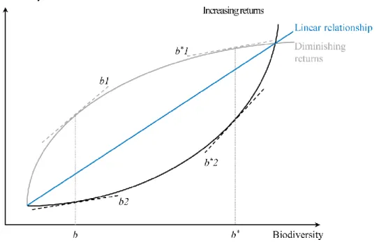
productivity as an example. Figure 10 gives a graphical depiction of a linear relationship alongside two others with increasing and diminishing returns. In a linear relationship, the influence of biodiversity on agricultural productivity is constant and equal to the slope of the line. In the non-linear relationships, this marginal influence is equal to the slope of the

(31)

marginal influence is equal to the slope of tangent line b2, and thus less than that of the linear relationship. However, for biodiversity value b*, this is exactly the other way around, that is to say, in the case of the diminishing returns relationship, the marginal influence (slope of tangent line b*1) is less than that of a linear relationship, while in the case of increasing returns it is greater (slope of tangent line b*2) than that of a linear relationship.

In conclusion, when the relationship between intermediate ecosystem services and final ecosystem services is non-linear, our assumption of a linear relationship may lead to both over- and underestimates of the growth rate of final services. To be able to say something realistic about the suitability of intermediate services as an indicator for final services, it is therefore crucial to gain insight into the functional relationship between ecosystems and the services they provide, and into the current situation, in other words, the point which the system has reached at this moment.

Figure 10. Illustration of relationships between biodiversity (Ei_{) and agricultural} productivity (Ef_{): linear, with increasing returns, with diminishing returns}

6.3 Production functions with tipping points and hysteresis

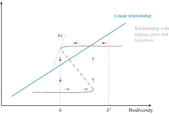
In cases where deviations from a linear relationship are minor, the assumption of a linear relationship will still lead to slight errors in the estimates of marginal effects on final ecosystem services. But deviations from linearity can be considerable, such as those in relationships characterised by tipping points and hysteresis, in other words, relationships typified by a transition between two stable states. Figure 11 gives an illustration of this kind of relationship.

(32)

Figure 11. Illustration of a relationship between biodiversity (Ei_{) and agricultural} productivity (Ef_{) characterised by a tipping point and hysteresis}

Suppose that a decline in biodiversity occurs. At value b*_{this clearly has no impact on}

agricultural productivity, nor, therefore, on welfare. At point b, a decline in biodiversity brings about a very abrupt, dramatic effect (slope of line segment b1), the system undergoes a shift and reaches a new equilibrium with significantly lower productivity (red arrows). What is problematic in this system is that it is difficult to return from this new, low-productivity equilibrium to the former equilibrium with high low-productivity (hysteresis; green arrows). In the most extreme case, not the situation depicted in Figure 11, recovering the former equilibrium is even impossible (irreversibility). The graph also reveals that, over a wide range of biodiversity values, marginal declines do not bring on changes in the relative scarcity of soil productivity and are therefore apparently not critical. This view does not make a correction for the fact that every marginal drop brings the system closer to a tipping point. If the location of such a tipping point is known, approaching it does not necessarily directly lead to problems, as long as it is possible to avoid actually reaching it in a timely manner. In practice, however, the presence and location of tipping points is very uncertain, which means that any marginal decrease (in biodiversity) increases the risk of marked negative effects on welfare. Still, from the dynamics of the ecological system, it can be deduced that we are approaching a tipping point. Increased dynamics in the system may hint at this and are therefore labelled as an early warning signal (see Scheffer et al., 2009). In cost-benefit analyses, it is extremely important to include both the direct effects on welfare and the risk of far-reaching effects in the future.11_{In these cases, it is possible to incorporate a}

precautionary principle in the cost-benefit analysis, even though it is not clear under what circumstances, and the principle itself is only vaguely defined.

6.4 Concluding remarks

Relative price increase for nature and ecosystem services