contact: H.Visser RIVM-MNP / IMP Hans.Visser@rivm.nl
RIVM report 550002007/2005
The significance of climate change in the Netherlands An analysis of historical and future trends (1901-2020)
in weather conditions, weather extremes and temperature-related impacts
H. Visser
This investigation has been performed by order and for the account of RIVM, within the framework of project S/550002/01/TO, Uncertainties, Transparency and Communication: Tools for Uncertainty Analysis.
A
BSTRACT
The significance of climate change in the Netherlands An analysis of historical and future trends (1901-2020)
in weather conditions, weather extremes and temperature-related impacts
A rigorous statistical analysis reveals changes in Dutch climate that are statistically significant over the last century. Annually averaged temperatures have increased by 1.5±0.5 ºC; the number of summer days has roughly doubled from 14±5 to 27±9 days; annual precipitation has increased by 120±100 mm; and the number of extremely wet days has increased by about 40%, from 19±3 to 26±3 days. Several other changes in Dutch climate, such as spring temperatures rising more rapidly than winter temperatures, the increase of the coldest temperature in each year by 0.9 ºC and the annual maximum day sum of precipitation, turn out to be not (yet) statistically significant.
The changes in Dutch climate have already led to several statistically significant impacts. The length of the growing season has increased by nearly a month, and the number of heating-degree days, a measure for the energy needed for the heating of houses and buildings, has decreased by 14±5%. Projections of future temperature continue to increase up to the year 2020, based both on statistical extrapolations and climate-model projections. It is found that temperatures increase from 10.4±0.4 ºC in 2003 to 11.1±0.6 ºC in 2010, and 10.8±1.0 ºC in 2020. Therefore, energy needed for heating of houses and buildings will decrease whereas energy for cooling will increase. The net climate effect in 2010 is expected to be a lowering of future Dutch greenhouse-gas emissions by 3.5 Mton CO2 equivalents, which is relevant in
the context of commitments under the Kyoto Protocol.
Finally, over the course of the 20th century the chance on an ‘Elfstedentocht’, an outdoor skating event in the Netherlands, has decreased from once every five years to once every ten years. Even though this impact change is not yet statistically significant, it resides ‘on the edge’ of significance: within a few years more evidence may become available to firmly establish the diminishing likelihood of outdoor skating in the Netherlands.
The ‘Elfsteden’ indicator is defined as the average temperature of the coldest period of 15 consecutive days in a specific winter.
-16.0 -12.0 -8.0 -4.0 0.0 4.0 'Elfsteden' indicator It (°C) 0.00 0.05 0.10 0.15 0.20
'Elfstedentocht' not organized
density
Probability density function 1901 Probability density function 2004 'Elfstedentocht' is organized
R
APPORT IN HET KORT
De significantie van klimaatverandering in Nederland Een analyse van historische en toekomstige trends (1901-2020)
in het weer, weersextremen en temperatuur-gerelateerde impact-variabelen
Statistische analyse van het Nederlandse weer laat veranderingen zien die reeds statistisch significant zijn, gezien over de afgelopen honderd jaar. Jaargemiddelde temperaturen zijn toegenomen met 1.5±0.5 °C sinds 1901. Het aantal zomerse dagen is ruwweg verdubbeld, van 14±5 naar 27±9 dagen. De jaartotale neerslag is toegenomen met 120±100 mm, en het aantal extreem natte dagen is met circa 40% toegenomen, van 19±3 naar 26±3 dagen. Andere onderzochte variabelen blijken niet significant te zijn veranderd, zoals de koudste dag per jaar en de maximum dagsom voor neerslag per jaar. Verder blijken de jaarlijkse temperatuur- en neerslagveranderingen homogeen over de maanden van het jaar verdeeld te zijn. Getalsmatig zijn er wel verschillen per maand of per seizoen, maar die blijken niet significant.
De veranderingen in het Nederlandse klimaat hebben reeds geleid tot significante veranderingen in weergerelateerde impact-variabelen. Zo is de lengte van het groeiseizoen toegenomen met bijna een maand, en het aantal graaddagen per jaar, een maat gerelateerd aan ruimteverwarming, is afgenomen met 14±5 %.
Projecties van temperatuurveranderingen voor het jaar 2020 die gebaseerd zijn op statistische extrapolatie vanuit het verleden, zijn consistent met voorspellingen op basis van klimaatmodellen. Gevonden is dat de jaargemiddelde temperatuur in Nederland zal toenemen van 10.4±0.4 °C in 2003 naar 10.7±0.6 °C in 2010 en 11.1±1.0 °C in 2020. Hierdoor zal in de toekomst minder energie nodig zijn voor ruimteverwarming maar meer voor koeling. Dit klimaateffect zal zeer waarschijnlijk de projecties van CO2-emissies tot aan het jaar 2012
doen dalen met 3.5 Mton CO2-equivalenten, een resultaat dat relevant is voor de Nederlandse
Kyoto-verplichtingen.
Tenslotte is onderzocht hoe de kans op een Elfstedentocht beïnvloed is door klimaatverandering. Het is gebleken dat de kans op een tocht aan het begin van de twintigste eeuw lag op 0.2, ofwel gemiddeld eens per vijf jaar. Deze kans is, na een toename tot 1950, afgenomen naar een kans van 0.10 in 2004, ofwel een gemiddelde terugkeertijd van eens per 10 jaar. De veranderingen liggen op de grens van statistische significantie. Binnen een klein aantal jaren zal blijken of de gevonden veranderingen inderdaad systematisch zijn.
Preface
Thanks goes to Jok Tang (TU Delft) who analysed a large number of climate indicators in the Netherlands. The analyses presented here, are a continuation of his work (Tang, 2003).
Albert Klein Tank, Adri Buishand and Theo Brandsma, all of KNMI, are thanked for their discussions on the reliability of weather data in the Netherlands, and for reviewing this report. Futhermore, Theo Brandsma kindly supplied the ice thickness data for the province of Friesland.
Arthur Petersen and Anton van der Giessen (both MNP/RIVM) are thanked for their thorough comments on earlier versions of this report.
Contents
SUMMARY...9 1. INTRODUCTION ... 11 1.1 GOALS... 11 1.2 HISTORICAL DATA... 13 1.3 FUTURE PROJECTIONS... 13 1.4 STATISTICAL APPROACH... 15 1.5 THIS REPORT... 152. DATA AND META DATA ... 17
2.1 TEMPERATURE... 17
2.1.1 Main observatory at De Bilt ... 17
2.1.2 Spatially averaged temperature record... 20
2.1.3 Global temperatures... 22
2.2 PRECIPITATION... 24
3. ESTIMATION AND DETECTION OF TRENDS ... 29
3.1 FLEXIBLE TRENDS... 32
3.2 EXAMPLE... 33
3.3 STRUCTURAL TIME-SERIES MODELS... 35
3.3.1 Model structure ... 35
3.3.2 How to choose the flexibility of the trend? ... 38
3.3.3 Predicting future data ... 38
3.4 SOFTWARE... 40
4. ANNUAL MEANS AND ANNUAL CYCLES ... 41
4.1 TEMPERATURE... 41
4.1.1 Annual means ... 41
4.1.2 Annual cycle ... 43
4.1.3 Are the results consistent with seasonal estimates? ... 45
4.2 PRECIPITATION... 47
4.2.1 Annual totals ... 47
4.2.2 Annual cycle ... 49
4.2.3 Are the results consistent with seasonal estimates? ... 51
5. EXTREME WEATHER CONDITIONS... 53
5.1 TEMPERATURE... 53
5.1.1 Absolute minimum temperatures ... 53
5.1.2 Absolute maximum temperatures... 56
5.1.3 Number of summer days ... 58
5.2 PRECIPITATION... 61
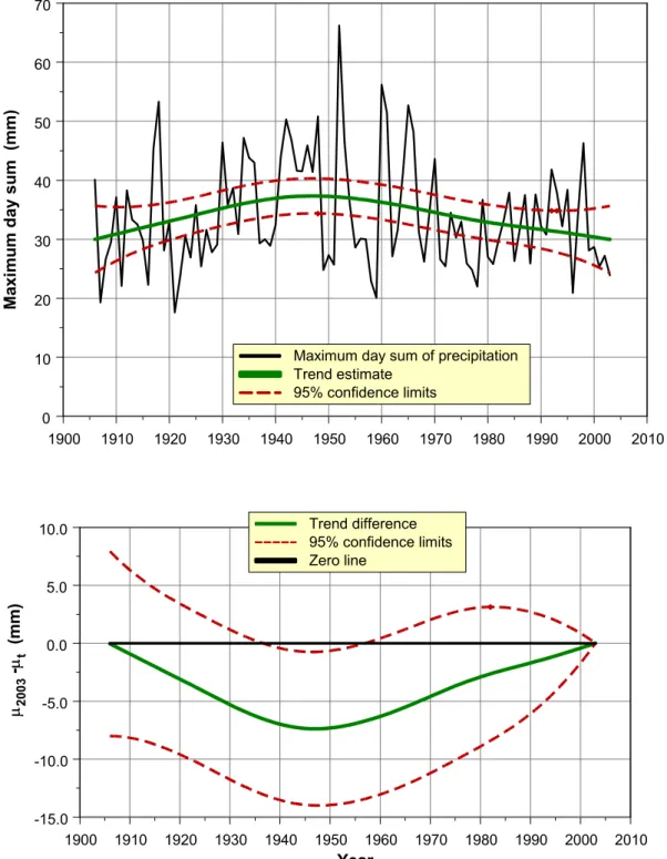
5.2.1 Maximum daily precipitation ... 61
5.2.2 Number of extremely wet days... 64
6. TEMPERATURE-RELATED IMPACTS ...71
6.1 PREMATURE DEATHS DURING HEAT WAVES...71
6.1.1 Low estimates...73
6.1.2 High estimates...73
6.1.3 Combination of estimates...76
6.1.4 Fewer premature deaths in winter ...76
6.2 CHANGES IN THE START OF THE GROWING SEASON...77
6.3 HEATING- AND COOLING-DEGREE DAYS...81
6.3.1 Heating-degree days ...81
6.3.2 Cooling-degree days ...83
6.4 OUTDOOR SKATING AND THE ‘ELFSTEDENTOCHT’ ...85
6.4.1 History...85
6.4.2 Indicator for maximum ice thickness...87
6.4.3 Trend estimate ‘Elfstedentocht’ indicator...89
6.4.4 Chance for an ‘Elfstedentocht’ ...91
7. FUTURE WEATHER CONDITIONS: A TWO-WAY APPROACH...95
7.1 PREDICTING GLOBAL WARMING UP TO 2020 ...98
7.2 PREDICTING LOCAL WARMING UP TO 2020 ...100
7.3 CONSEQUENCES FOR WEATHER-RELATED INDICATORS...105
7.3.1 Heating-degree days ...106
7.3.2 Premature deaths ...110
8. SUMMARY AND CONCLUSIONS...111
REFERENCES ...119
Appendix A Comparison of historical station data ...125
Appendix B Wind ...133
Appendix C Global and local climates are connected ...141
S
UMMARY
Recently, the Dutch Parliament raised the Commission Climate Change. This commission poses the following questions, among others: (i) what are actual insights and dimensions of climate change for the Netherlands, (ii) how should uncertainties be judged, (iii) what can we expect for the near future, and (iv) what policy measures should be taken to mitigate adverse societal and economical consequences of climate change? This report is directed to the first three questions.
The method applied here is that of a rigorous time-series analysis, applied to a set of homogenized weather data in the Netherlands (non-homogeneized data are characterized by changes in instrumentation, changes in the height of an instrument, changes in location of the instrument and/or changes in the environment of the instrument). The time-series approach is based on Structural time series analysis and the Kalman filter. This approach yields, apart from flexible trend estimates, uncertainties for changes in the trend estimates.
Results reveal that a number of daily temperature and precipitation series can be regarded as homogeneous over the period 1901-2003. However, series for wind speed and wind direction were not reliable enough for trend analyses. Subsequently, the latter data have not been analysed.
Statistical trend analyses reveal changes in Dutch climate that are statistical significant over the last century: annual temperatures have increased by 1.5±0.5 °C, annual precipitation sums by 120±100 mm. The length of the growing season has increased by nearly a month, and the number of heating-degree days, a measure for the energy needed for the heating of houses and buildings, has decreased by 14±5%. Over the course of the 20th century the chance on an ‘Elfstedentocht’, an outdoor skating event in the Netherlands, has decreased from once every five years to once every ten years. Even though this impact change is not yet statistically significant, it resides ‘on the edge’ of significance.
Statistical extrapolation of future temperatures shows to be consistent with projections based on GCM calculations. Temperatures will continue to increase from 10.4±0.4 ºC in 2003 to 10.7±0.6 ºC in 2010 and 11.1±1.0 ºC in 2020. As a consequence, emissions of CO2
equivalents for the year 2010 are likely to be 3.5 Mton lower than is to be expected on economic grounds and a stable climate for the near future.
The trends identified clearly show the need for policy measures to mitigate the consequences of climate change. The projected warming and subsequent increase in extreme weather conditions will have significant societal impacts, even on the short term.
1.
Introduction
1.1
Goals
What are the actual insights and dimensions of climate change for the Netherlands, and to what extent are these caused by the greenhouse effect? How should uncertainties be judged? What policy measures should be taken in the near future, and what will be the societal, economic and environmental implications of these measures? These represent the main questions recently posed by the Dutch Parliament to the Commission Climate Change.
The report before you will focus on the first three questions raised above, concerning actual insights and dimensions of climate change for the Netherlands and ways to judge uncertainties. More specifically, the following questions are dealt with.
− What are the trends in weather conditions in the Netherlands over the past century? What is the uncertainty in these trends?
− Have there been shifts in the frequency of extreme events such as heat waves or droughts? To what extent are these shifts certain/uncertain?
− What are societal impacts of weather conditions or weather extremes? How have these impacts evolved over the past century?
− Is it permissible to extrapolate trends in weather conditions over the past century to the near future, i.e. the years up to 2020?
− If so, what should we expect in the 16 years ahead? And what are the uncertainties in these projections?
As for changes in weather conditions, trends are often presented for annual averaged temperatures or annual totals of precipitation. These series have been published in numerous publications, such as IPCC (2001) and the references contained. Annual series in the Netherlands can be found in KNMI (2003) and MNP (2003, 2004).
Of equal importance are extreme weather conditions. In fact, societal implications of weather extremes are much more severe than changes in annual averages. Because of the importance of extremes, the European Climate Support Network (ECSN) took the initiative in 1998 for a European Climate Assessment (ECA) project. Key questions were ‘how did the past
warming affect the occurrence of temperature extremes’ and ‘was the past warming accompanied by a detectable change in precipitation extremes’? The Royal Netherlands
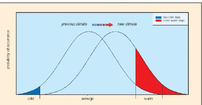
Meteorological Institute (KNMI), coordinator of the project (Klein Tank et al., 2002a; Klein Tank, 2004), has pointed out that small shifts in annual averages may lead to disproportionate shifts in the chance of extreme events, making the study of extremes even more important. This aspect is illustrated in Figure 1.1.
On the one hand, this report answers the same questions as posed by the KMNI project, although only for the Netherlands, but on the other, questions on ‘how weather-related impacts evolved’ and ‘what future developments are expected up to 2020’ are also answered. As for weather-related impacts, only a limited number of situations are dealt with here: (i) the influence of warm periods on premature deaths, (ii) shifts in the onset of the growing season, (iii) the influence of climate change on the number of heating-degree days and (iv) the effect of global warming on the chance of maintaining outdoor skating, a sport very popular in the Netherlands.
A number of impacts are not dealt with here, such as: forest fires, extension of the hay fever season, storm damage, bad harvests due to drought or due to large amounts of rain in a few days time, and flooding of the Meuse and Rhine. Positive impacts could be: increasing harvests due to prolonged growing season, winegrowing and tourism. An even larger set of impacts has been defined in EEA (2004) and impacts are described in a more popular form in a special issue of National Geographic (2004a,b).
Figure 1.1 Schematic effect on the number of cold and warm days for a ‘symmetric’ increase in the mean temperature. Source: Klein Tank et al. (2002a).
1.2
Historical data
We are very fortunate in the Netherlands to have a large number of historical time series available. Recently the KNMI published a number of series extending back to the 18th and 19th centuries, all data measured before the start of the KNMI in the year 1854 (this year is the 150th anniversary of the institute!). However, the use of these historical data is limited for use in long-term trends, as is explained below. For the analyses reported here, 1901 was chosen as the initiation year, although many data prior to this date are available. Here, 1901 is the starting year of the main observatory at location De Bilt.
The reason for limiting the use of these data is our uncertainty on the homogeneity of these series influenced by:
− changes in instrumentation
− changes in the height of an instrument − changes in locations of instruments and
− changes in the surroundings of the stations, such as the growth of trees.
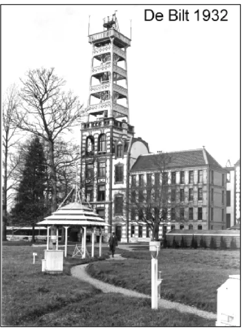
The main source of data was the main observatory of KNMI in De Bilt, as shown in Figure 1.2. The photo shows an open pagoda type of screen, a pluviograph hut just in front of the pagoda and, more to the right, the open precipitation instrument, which has been manually recorded every day at 8.00 hours since 1901.
1.3
Future projections
As for future data, a robust approach has been chosen, in which weather conditions are predicted in two-ways: one method is based on GCM predictions for both natural and anthropogenic warming, the other method is purely based on historical data.
The simple idea behind this two-way approach is that one can be more confident in future developments if two independent approaches yield similar and consistent results. Futhermore, it is generally felt amongst climatologists that future trends are best predicted by GCMs, while the year-to-year variability is best captured by analysing historical data. The latter variability is not capture good enough by GCMs with their inherent uncertainties and large grid sizes.
Figure 1.2 Main KNMI observatory in De Bilt in a photo taken around 1932.
Shown are the pagoda type of measurement screen (to the left, in front of the tower) and the rain gauge (to the far right up front). Photo: KNMI.
1.4
Statistical approach
An important aspect of the approach followed here concerns the statistical treatment of
trends. There are many methods available for estimating (flexible) trends in data. However,
the number of suitable methods are limited if one is interested in estimates for uncertainty. Why is uncertainty important within this context? Suppose some weather-related variable xt
has a value of 9.0 in 1901 and 10.0 in 2003. It is tempting to conclude in this case that this variable has increased over a century. However, if the year-to-year variability follows a normal distribution with a standard deviation of 0.5, the 95% confidence limits are ±1.0. In other words, x1901 = 9.0 [8.0, 10.0] and x2003 = 10.0 [9.0, 11.0]. Clearly, uncertainties are too
large for drawing inferences on significant increases. At best, one could conclude that there is a tendency to increase. More data are needed to prove the significance of this tendency (in most cases confidence limits become narrower as more data become available).
Visser (2003; 2004) has presented an approach in which three trend-derived uncertainties are estimated, the most notable of which is the uncertainty in the trend estimate in the final year relative to trend estimates in all preceding years. This approach is followed throughout this report.
1.5
This report
The report will continue in Chapter 2 to describe the data and meta data, i.e. the history of stations and instrumentation. The statistical approach is given in Chapter 3 , while Chapter 4 analyses trends of annually averaged temperatures and annual sums of precipitation. The yearly cycle for precipitation is given as well. Chapter 5 is devoted to a select number of extreme weather indicators, such as the coldest and hottest moments in a year, or the maximum number of consecutive dry days. Chapter 6 deals with four temperature-related impact variables, such as the number of premature deaths during warm summers.
Subsequently, there is a switch to future climate change in Chapter 7. Here it is verified if trends estimated over the 1901-2003 period can be extrapolated to the 2004-2020 period. Chapter 8 brings the report to a close with the conclusions.
The report ends with three Appendices giving details not mentioned in the main text. For policy purposes a special Appendix has been inserted giving predictions for heating- and cooling-degree days over the period 2004 - 2040.
2.
Data and meta data
The origin of the weather record used throughout this report is described here, along with the history of the series, i.e. the meta data. Because the goal here is to detect changes over more than a century’s time, we have to be very careful for inhomogeneities, inducing false trends. For example, if a temperature record shows a warming trend over the 1901-2003 period, it is easy to make inferences on climate warming, possibly due to the enhanced greenhouse effect. However, such warming could be (partially) caused by urbanization in the surroundings of the station. Thus, the effect of urbanization should be dealt with in temperature records. Other sources of inhomogeneity are relocations of the station, changes in the height of the instrument, changes in the type of instrument, and changes in the station surroundings, such as tree growth.
Temperature records will be covered in section 2.1, precipitation sums in section 2.2. Conclusions are drawn in section 2.3. Records of windspeed and wind direction are treated in Appendix A. Because of a lack of homogeneity these records fall short. For applications on relative short time series (1961 onwards) the reader is referred to KNMI (2003, p. 14) and Smits, Klein Tank and Können (2004).
2.1
Temperature
2.1.1 Main observatory at De Bilt
The station called De Bilt (52.10 ˚N, 5.18 ˚E, 2.0 m) is representative of the mean climate conditions in the Netherlands (see Figure 1.2). Its temperature series is considered to be the most homogeneous long-term record of the Netherlands. The daily mean temperature series for De Bilt, from 1901 to date is available from the KNMI website and the European Climate Assessment data set (Klein Tank et al., 2002, www.knmi/samenw/ECA). Series can also be downloaded from the KNMI website (www.knmi.nl/product). Click on [English] and choose data in the upper panel on the page). The meta data can be found on this website as well. The monthly means of this series have recently been homogenized by Brandsma (Brandsma
et al., 2003) for the effects of a relocation and change of the thermometer screen in 1950,
another relocation in 1951, the lowering of the screen from 2.20 m to 1.50 m in 1961 and urbanization effects. For the 1951-1970 period the monthly mean temperature is now derived from hourly ‘climatological measurements’. The ‘synoptic measurements’− which, for
practical reasons, have been used up to now for that period − are inferior in quality. The size of these corrections is about 0.2 K; a few months in the 1950-1960 period have corrections of more than 0.4 K. Changes in the measurement screen in 1980 (wood to plastic) and 1993 (Stevenson to unventilated saucer) have not yet been corrected for, but these corrections are estimated to be much smaller. The need for an urbanization correction is illustrated in Figure 2.1.
Figure 2.1 Land-use changes from the year 1900 (left panel) to the year 2000 (right panel).
The five main observatories are also shown in the maps. Three observatories were moved to an airport nearby. Legend is (from top to bottom): grassland, crops and bare ground, heathland and high moorland, deciduous forest, coniferous forest, built-up areas and roads, water, reedy swamps, shifting dunes and sandbars, other uses. Source: HGN database, Alterra (www.hgnnederland.nl).
Maastricht Beek Den Helder Vlissingen Vlissingen De Kooy Eelde Groningen De Bilt De Bilt
The degree of urbanization (the red areas in the figure) has strongly increased since 1900 (left panel). De Bilt is located just east of the city of Utrecht, which grew immensely in the last century. Brandsma derived a correction factor for annual averaged temperatures of 0.10 ± 0.06 K, which is in fact relatively small.
A number of analyses in this report are based on daily data rather than monthly averages. To use the improvements found by Brandsma, each daily temperature (daily average, daily maximum and daily minimum temperature) was adjusted using the correction factors found by Brandsma for the monthly averages. In this way we three semi-homogeneous daily records could be constructed. However, it should be noted that daily minimum and maximum temperatures are more sensitive to changes in the height of thermometers (Brandsma found for the lowering of an instrument from 220 cm to 150 cm, that the daily cycle will increase by 0.33 K).
There is only one situation where we have to be careful, i.e. the warmest moment of a year (section 5.1.2). This indicator is very sensitive to type of screen. The open pagoda type of screen, used from 1901 to 1950, will tend to give temperatures that are somewhat too high on sunny days with low wind speeds (see Figure 2.2). Under these circumstance the air under
Figure 2.2 Pagoda type of measurement screen at De Bilt.
The photo left shows an interesting detail: a Stephenson cabin to the right of the pagoda screen. Temperature recordings from this screen would be useful for homogenization purposes. However, according to the station manager these recordings were lost, probably due to reductions in archive space... The photo on the right shows the thermograph along with min-max thermometers.
the roof of the ‘pagoda’ will be heated by sunlight reflected by the ground around the screen, creating, in fact, a ‘micro greenhouse effect’.
2.1.2 Spatially averaged temperature record
At the start of the 20th century five major observatories were erected. These were Den Helder, Groningen, De Bilt, Vlissingen and Maastricht. Their locations are given in Figure 2.1. The stations were chosen the ‘corners of a rectangle’, with De Bilt situated around the crossing of the diagonals of this rectangle. The stations are shown in Figure 2.3. Daily data can be downloaded from www.knmi.nl/samenw/ECA.
The stations Den Helder, Groningen and Maastricht have been moved to airports nearby: De Kooy, Eelde and Beek, respectively. The influence of these movements on homogeneity is shown for annual averaged temperatures in the scatter-plot matrix in Figure 2.4. The scatter plots show two parallel lines for Maastricht station. It has been verified that one line corresponds to the 1901- 1972 period (Maastricht) and the other line to 1973-2003 (Beek). Therefore, Maastricht/Beek has been omitted for a check on homogeneity at the De Bilt station.
A comparison between the De Bilt record and the four-station mean records is given in Figure 2.5. The upper panel shows the scatterplot between each series. The graph shows a good correspondence between both series (R = 0.99), with results indicating, from a different angle, that the homogenized De Bilt series is reliable for use in trend analyses.
Graphs analogous to Figure 2.5, are shown in Appendix A for the indicators treated in Chapter 5. These indicators are: absolute minimum and maximum temperatures, number of summer days, maximum daily precipitation, number of extreme wet days and the maximum number of consecutive dry days.
Figure 2.3 From top to bottom: the stations of Den Helder - De Kooy (moved in 1972), Groningen - Eelde (moved in 1946), Maastricht - Beek (moved in 1946) and Vlissingen (moved in 1945, 1947 and 1958 in the Vlissingen area).
1972 1946 1945 1947 1958 1946
Figure 2.4 Scatterplot matrix for annual averaged temperatures at De Bilt, Den Helder, Groningen, Vlissingen and Maastricht. Scatterplots for the average of these five stations are also shown.
2.1.3 Global temperatures
The global temperatures used in this report are taken from Jones et al. (2001). Data can be downloaded from www.cru.uea.ac.uk/cru/data/temperature. For discussions on the construction and homogeneity of this series please refer to Jones (2001) and references contained. The series was extensively used in IPCC (2001).
Tg.DeBilt 8 9 10 11 8 9 10 11 8 9 10 11 8 9 10 11 8 9 10 11 Tg.DenHelder Tg.Groningen 7 8 9 10 8 9 10 11 Tg.Vlissingen Tg.Maastricht 8 9 10 11 8 9 10 11 8 9 10 11 7 8 9 10 8 9 10 11 Tg.Mean.5.stations
Figure 2.5 Time series of annual temperatures for the De Bilt station (green line) and annual averages of four stations (Den Helder, Groningen, De Bilt and Vlissingen; orange line). The lower panel shows the scatter plot between both series.
The correlation coefficient is 0.99. Period is 1906 – 2003.
8.0 9.0 10.0 11.0
Annual temperatures 4 stations (°C)
8.0 9.0 10.0 11.0 An n u al tem p eratu res stati o n D e Bi lt ( °C) R= 0.99 1900 1910 1920 1930 1940 1950 1960 1970 1980 1990 2000 2010 Year 7.0 8.0 9.0 10.0 11.0 A n n u al temp eratu res ( °C) Average of 4 stations Station De Bilt
2.2
Precipitation
Within the ECA project 13 stations in the Netherlands were homogenized over the 1901-2003 period (Klein Tank et al., 2002b). Station names are, from north to south: West Terschelling, Groningen, Den Helder, Ter Apel, Hoorn, Heerde, Hoofddorp, De Bilt, Winterswijk, Kerkwerve, Oudenbosch, Axel and Roermond. All these stations were corrected for a lowering of the instrument from 2.0 m to 0.50 m (Bruin, 2002). As homogeneity tests can be found on the ECA website, they are not repeated here. See Figure 2.6.
The daily time series are all taken from the manual network. Within this network precipitation is recorded by an observer every day at 8.00 hours (Figure 2.7). An important advantage of measurements taken manually over automated stations using pluviographs is that long-term trends in the latter series may be biased due to calibration errors, changes in types of pluviographs, and incidental influences of leaf fall, hail and snow.
Errors in manual measurements on the other hand will be random rather than systematic (bias). Readings from the observer may be incidentally too high or too low, or sometimes somewhat before or after 8h.00 or even forgotten for one day. However, by taking precipitation sums over months or years these errors will average out. For more detailed information the reader is referred to Buishand and Velds (1986) and Bruin (2002).
The annual totals of precipitation for De Bilt and the 13-station records are compared in Figure 2.8. Both series appear to be very similar. The correlation coefficient is R = 0.94, a relatively high value, signifying the fact that though precipitation is a phenomenon which occurs on more local scales than temperature, this locality is largely smoothed out on a yearly basis.
Figure 2.6 Map of the Netherlands showing 283 precipitation stations, divided over 15 precipitation districts.
All stations have been in operation since 1970. The stars refer to the 13 stations used in this report.
Figure 2.8 Time series of annual precipitation sums for De Bilt (green line) and the annual sums of 13 stations (location given in Figure 2.6; see orange line). The lower panel shows the scatter plot between each series.
The correlation coefficient is 0.94 and the period covers 1906 – 2003.
1900 1910 1920 1930 1940 1950 1960 1970 1980 1990 2000 2010 Year 400 600 800 1000 1200 1400
Annual precipitation De Bilt Annual precipitation for 13 stations
An n u al p reci p itati o n su m s (mm ) 400 600 800 1000 1200 1400
Annual precipitation for 13 stations (mm)
400 600 800 1000 1200 1400 An n u al p reci p itati o n fo r stati o n De B il t (mm) R = 0.94
3.
Estimation and detection of trends
In this chapter a trend estimation approach is introduced which allows the estimation of flexible trends with corresponding uncertainty information on the trend itself and trend increments. The latter information is important for the question: is the final trend estimate larger or smaller than some trend estimate in the past, given the uncertainty (‘noise’) in the data? The importance of such information is illustrated in the inset (9 > 10 ??!!).
The methodological aspects of estimating flexible trends (versus linear trends) will be given in section 3.1, and clarified by an example in section 3.2. Section 3.3 gives a concise summary of the mathematical formulation of the trend models used throughout this report, and section 3.4 describes the corresponding TrendSpotter software.
Systematic treatment of uncertainties in trend estimates is essential for drawing robust inferences on climate change.
A general framework for dealing with uncertainties is given in Petersen et al. (2003). Photo: H. Visser.
9 > 10 ??!!
The trend models throughout this report are taken from the class of structural time series
models. The rationale is not that these trend models are necessarily better than other trend
models, such as moving averages or splines, but that uncertainty information is easily gained. Why is such uncertainty information important? We will illustrate this by a hypothetical example showing that two measurements or estimates X and Y do not necessarily follow the standard calculation rules. Of course, 9 < 10, but is it possible that 10 < 9? The answer is ‘yes’ if both variables have measurement or modelling errors.
Suppose the errors in X and Y follow normal distributions with expectations 9.0 and 10.0, respectively. As variances we choose 0.42 for X and 0.52 for Y. In statistical notation: X ≈ N(9.0, 0.16 ) and Y ≈ N(10.0, 0.25). Both probability density functions are shown in Figure 3.1A. The figure shows that there is a (small) chance that X > 10.0: P(X > 10.0) = 0.6%, and a chance that Y < 9.0: P(Y < 9.0) = 2.3%. Thus, there is a chance that X > Y, although their expected values are 9.0 and 10.0, respectively.
The chance that X > Y follows from the distribution of Z: Z = Y – X. If X and Y are mutually independent, it follows Z ≈ N( 1.0, var(X) + var(Y)) , or Z ≈ N(1.0, 0.41). The
Figure 3.1A Normal probability density functions of X and Y.
7.0 8.0 9.0 10.0 11.0 12.0 X 0.0 0.2 0.4 0.6 0.8 1.0
Normal density function for X Idem for Y
Y
probability function of Z is shown in Figure 3.1B (black line). It is found that P(Z < 0.0) = 5.9%.
However, the variables may be correlated, for example with a correlation coefficient of R = 0.70. Now, the variance of Z will be smaller:
Z ≈ N( 1.0, var(X) + var(Y) – 2.0*cov(X,Y)) , or Z ≈ N(1.0, 0.21)
The probability function of Z is also shown in Figure 3.1B (blue line). Now, it is found that P(Z < 0.0) = 1.5%.
This hypothetical example shows that measurements or model outputs do not always follow traditional calculation rules. Although the expectation of Y is larger than that of X, it can be found that X > Y, in the examples above with a chance of 5.9% and 1.5%.
In this report the variable X can be seen as a trend estimate for some historic year t (µt), with
1900 < t < 2003, and Y as the trend estimate for the year 2003 (µ2003). If we want to draw
inferences on trends, we have to know the probability distribution of the difference Z = µ2003 - µt. Here, the variables µ2003 and µt are typically correlated. The distribution of Z
follows from Kalman filter theory (Visser, 2004). The importance of having significance limits for the trend differences µ2003 - µt has been demonstrated.
Figure 3.1B Probability density functions for the difference Z = Y – X.
-2.0 -1.0 0.0 1.0 2.0 3.0 4.0 Y - X 0.0 0.2 0.4 0.6 0.8 1.0
Variables mutually independent Variables correlated with R = 0.70
X > Y Y > X
3.1
Flexible trends
Many studies on trend estimation deal with linear or monotonously increasing/decreasing trends. For example, Hess et al. (2001) presented an overview of six statistical methods for this type of trend. However, not all trends in environmental applications behave in a more-or-less linear manner. If one analyses historical climate data such as temperatures or precipitation sums over a period of centuries, alternating periods of increase or decrease are seen, as well as periods where the variable is more-or-less constant. Linear trends do not give sufficient information for these kinds of situations and could even be misleading. Another situation where linear trends may lead to incorrect inferences, is that of data with strong serially correlated errors (Woodward and Gray, 1993 and 1995, and references in Visser, 2004, Appendix B).
If we are interested in the significance of a trend, there are also important differences between linear and flexible trend estimation. A test for a linear or monotonous trend will have only one answer − ‘yes’ or ‘no’. Or more formally, we either fail to reject the null hypothesis (H0)
of no trend, or reject it, given some choice for α. Here α stands for the chance of rejecting H0
while it is true in reality.
For example, one could choose the ordinary least squares (OLS) regression trend line (section 3.3 in Hess et al., 2001). The model is formulated as follows: yt = a + b*t + εt, where εt is a
white noise process. Here, the trend, µt, is defined as a + bt, with t = 1, … , N. The
significance of the trend follows directly from the variance σb2 of the slope b. If
-2*σb < b < 2* σb , the decision fails to reject the H0 hypothesis, and there is no significant
trend.
In the case of a flexible trend, the slope b becomes time-dependent and a single test on slope will no longer suffice. Now the variances of all possible trend differences, µt - µs could be of
interest. Since the presentation of all these differences is not practical, the following two functions of time will be useful:
• µt with corresponding 2*σt confidence limits, t =1, …, N. These limits are also calculated
in the case of the OLS regression trend.
• the lagged differences, µN – µt, with corresponding 2*σt confidence limits, t = 1, …., N.
The first function allows us to test significant differences at certain levels. The second function, with the form µN – µt, was chosen since, in practice, we are interested in how the
present (µN) deviates from the past (µt). Are present levels of temperature or precipitation
whether recent values are extraordinary or not. This wish is reflected in the choice of the function, µN – µt . N will be the year 2003 throughout this report.
The approach will be illustrated in the following by an example in section 3.2, and a short description of the mathematical background given in section 3.3. Software is described in section 3.3. For a more detailed description the reader is referred to Visser (2003; 2004).
3.2
Example
Figure 3.2 shows a series of annually averaged global temperatures over the 1901-2003 period (black line). The series is extensively used in publications such as IPCC (2001); compare this to section 2.1.3.1) It should be noted that the average global temperature over the 1960-1990 period has been subtracted from all annual data, leading to a ‘relative’ zero point.
From the upper panel it is clear that a linear OLS trend fit is not what the data reveals. There is a period showing increase (1901-1940), a period showing stabilization (1941-1970), and again, a period with increasing temperatures from 1971 onwards. A flexible trend µt with 2-σt confidence limits was therefore estimated. Limits may be interpreted as 95% confidence
limits (residuals of the model are normally distributed). The trend difference of µ2003 – µt is
given in the lower panel of Figure 3.2. Trend statistics are:
• µ1901 = -0.39 [-0.47, -0.31] ºC
• µ2003 = 0.45 [0.36, 0.54] ºC
• µ2003 - µ1901 = 0.86 [0.74, 0.98] K
• µ2003 - µ2002 = 0.020 [0.004, 0.036] K
The estimation results clearly show the gradually increasing temperatures over the 1901-1949 period, the stabilization from 1940 to 1970 and the acceleration of global warming afterwards. The trend value in 2003 is statistically larger than all trend values in the period of 1901-2002 (using α = 0.05, which corresponds to a two-sided test of significance, using the 95% confidence limits in the lower panel).
1) For this particular series it is known that early global temperatures are less reliable than values at the end of the series. The TrendSpotter software is not able to give weigths to individual measurements in its present form. The software will be extended with such a weighing option early 2005.
Figure 3.2 Analysis of the combined land, air and sea surface temperatures for the 1901-2003 period, relative to the 1960-1990 period.
Data are from Jones et al. (2001), University of East Anglia (CRU). The upper panel shows the data and the trend with 95% confidence limits. The lower panel shows the difference function of µ2003 – µt with 95% confidence limits. All differences are
above the zero line. In other words, the trend value in the final year, 2003, is significantly higher than all preceding trend values (given the choice of α = 0.05 and a two-sided test). 1900 1910 1920 1930 1940 1950 1960 1970 1980 1990 2000 2010 -0.6 -0.4 -0.2 0.0 0.2 0.4 0.6 Global temperatures Trend estimate 95% confidence limits An nual t emperatures relative to 1960-1990 ( °C) 1900 1910 1920 1930 1940 1950 1960 1970 1980 1990 2000 2010 Year -0.2 0.0 0.2 0.4 0.6 0.8 1.0 µ2003 - µt ( °C) Trend difference 95% confidence limits Zero line
3.3
Structural time-series models
3.3.1 Model structure
Only a few methods give some sort of confidence limits for trend estimates for the detection of flexible trends, here, the LOESS estimators, as described by Cleveland and Grosse (1991), polynomial regression fits (models of the form, yt = a + b*t + c*t2 + d*t3 + …. + εt ), and
trends from the class of structural time-series models. Confidence limits for the individual
trends estimates µt for the first two models are known from the literature. But, as far as we
know, no formulae have been derived for the first and lagged differences. However, such formulae have been derived for trends from the class of structural time-series models in combination with the Kalman filter (De Jong, 1988 and Visser, 1994).
There is a vast amount of literature on structural time-series models. The most important references, mainly from the field of econometrics, are Harvey (1984; 1989), and Durbin and Koopman (2001). Structural time-series models have a modular structure, with measurement, yt, at time, t, seen as an additive sum of four components:
yt = trendt + cyclet + influence of explanatory variables xt + noiset (1a)
or, more formally,
yt = µt + γt + α1,t * x1,t + α2,t * x2,t + … + εt (1b)
If the relationship between yt and its components is multiplicative rather than additive, a
logarithmic transformation of yt may be taken, i.e. yt’ = ln(yt + c) for a suitable constant c,
and ‘ln’, the notation for the natural logarithm. From equation (1) the model appears conceptually simple. Other transformations, such as the Box-Cox transformation, will not be taken up in the following chapters.
The trend model used for the examples in this report is called the integrated random walk
(IRW), suggested by Kitagawa (1981) and Young et al. (1991). This model was used with
environmental applications by Visser and Molenaar (1990; 1995), van den Brakel and Visser (1996), and Visser (2003). The trend model reads:
µt - 2µt-1 + µt-2 = ηt and yt = µt + εt (2a)
where ηt and εt are independent white noise processes with a zero mean, with respective
Model (2a) can be written in the so-called state-space form:
(
)
t t t t t t t t t y and ε λ µ η λ µ λ µ + = + − = + + 0 1 0 0 1 1 2 1 1 (2b) ) , 0 ( ) , 0 ( ση2 ε σε2 η N and N with t ≈ t ≈Other trend models from the class of structural time-series models are given in Visser (2004, Appendix B). The question on what model to choose, given a data set, is also dealt with. The cycle model γt in model (1b) is defined by
length period the S and N with t t S i t i (0, ) 2 1 0 γ =ω ω ≈ σω
∑
− = − (3)As a consequence of model (2a) we have the complete distribution of the trend µt and a
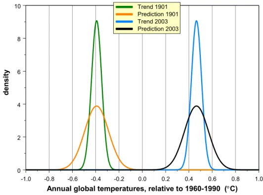
prediction of an observation ŷt. As an illustration we have plotted the normal density
functions for the estimates µ1901, ŷ1901 , µ2003 and ŷ2003 in Figure 3.3. The figure shows that
µ1901 << µ2003, being consistent with the findings in the lower panel of Figure 3.2.
The notation in state-space form is a necessary condition for estimating models (1) and (2) through use of the Kalman filter. This filter, designed by Kalman in 1960, has been used since in numerous applications. Where the noise processes, ηt and εt, in (2) are normally
distributed, the Kalman filter yields optimal estimates for the trend µt. In jargon, the filter
yields the Minimum Mean Square Estimator (MMSE) for the vector (µt , λt)’ from (2b), based
on observations up to and including time t. If the noise processes have a distribution other
than normal, the filter is still optimal, albeit somewhat less powerful. In the latter case the
filter generates the Minimum Mean Square Linear Estimator (MMSLE) for (µt , λt)’. These
Figure 3.3 Normal density functions for the estimates µ1901, ŷ1901 , µ2003, and ŷ2003 . Data are based on model estimates shown in Figure 3.2.
For more details on the Kalman filter, please refer to Harvey (1984; 1989, Chapter 3), and Durbin and Koopman (2001). A number of tests given by Harvey (1989, Chapter 5) have been applied here for diagnostic checks. For understanding the trend models presented in the following chapters, it will be essential to highlight one aspect of the estimation process in the next section, i.e. the flexibility of the trend.
-1.0 -0.8 -0.6 -0.4 -0.2 0.0 0.2 0.4 0.6 0.8 1.0
Annual global temperatures, relative to 1960-1990 (°C)
0 2 4 6 8 10 de ns ity Trend 1901 Prediction 1901 Trend 2003 Prediction 2003
3.3.2 How to choose the flexibility of the trend?
By varying the variances of the noise process, ηt, the flexibility of the trend can be set.
If ση2 = 0.0 is set, model (2) equals an OLS linear trend fit: a straight line. If ση2 is set to a
very large number, the trend will be passed on to all the measurements. Thus, ση2 will serve
as a ‘smoothing parameter’ in the model. But, what is the right choice for ση2 ?
To obtain an objective measure, ση2 is estimated by means of a maximum likelihood
optimization. In essence, this estimator tries to minimize the errors in the one-step-ahead predictions generated by the Kalman filter. The filter iteratively generates a trend prediction, µt+1’, based on all measurements y1, ….. , yt . This prediction µt+1’ is then compared to the
actual measurement, yt+1 , yielding the one-step-ahead prediction error or innovation
νt+1 = yt+1 - µt+1’. We now choose ση2 so that the sum of squared innovations νs2 + ….+ νN2 is
minimal (note that the summation starts at time step s, and not at time step 1, since the filter needs some iteration steps to converge; in practice, the filter has a start-up phase of between 10 and 20 time steps).
This is, in short, the rationale behind the maximum likelihood estimator. For details, please see Harvey (1989, section 3.4). The maximum likelihood estimation process has been applied throughout this report.
3.3.3 Predicting future data
The prediction of future data is part of the mathematical framework of structural time-series models and the Kalman filter (Harvey, 1989; Visser, 2003). This characteristic will be applied in Chapter 7 of this report. Here, we will give an example for the global temperature series of Jones et al. (2001), as presented in Figure 3.2.
We have estimated a trend model for the 1901–2020 period. The estimation results are shown in Figure 3.4 and the trend statistics below:
• µ1901 = -0.39 [-0.47, -0.31] ºC • µ2003 = 0.47 [0.39, 0.55] ºC • µ2010 = 0.61 [0.42, 0.80] ºC • µ2020 = 0.81 [0.39, 1.23] ºC • µ2020 - µ1901 = 1.20 [0.76, 1.63] K • µ2020 - µ2019 = 0.02 [-0.01, 0.05] K
Clearly, the trend is extrapolated linearly over the 2004-2020 period. Furthermore, the confidence limits in the upper panel show that the further we predict into the future, the wider the confidence limits become. The lower panel shows µ2020 to be significantly higher than all
trend values before the year 2000.
Figure 3.4 Analysis of the combined land air and sea surface temperatures for the 1901-2003 period, relative to the 1960-1990 period.
Estimates are extrapolated over the 2004-2020 period. Data are from Jones et al. (2001). The upper panel shows the data and the trend with 95% confidence limits. The lower panel shows the difference in function µ2020 – µt , with 95% confidence
limits. 1900 1910 1920 1930 1940 1950 1960 1970 1980 1990 2000 2010 2020 -0.6 -0.4 -0.2 0.0 0.2 0.4 0.6 0.8 1.0 1.2 Global temperatures Trend estimate 95% confidence limits An nu al te mpera tu res r elative to 19 60 -1 99 0 ( °C) 1900 1910 1920 1930 1940 1950 1960 1970 1980 1990 2000 2010 2020 Year -0.2 0.0 0.2 0.4 0.6 0.8 1.0 1.2 1.4 1.6 1.8 µ2003 - µt (° C)
3.4
Software
There is not much software on structural time-series models. And this may explain why this class of models is not as widely applied as the ARIMA models, for example. The main software implementation is the Structural Time-series Analyser, Modeller and Predictor (STAMP, in short), distributed by Timberlake Consultants LTD. Information can be found on the websites: http://stamp-software.com and http://www.timberlake.co.uk
The TrendSpotter software was initially developed at KEMA, but since 2001 at the RIVM. All examples in this report have been calculated using this software package, written in Fortran and running on a standard PC. Computation results are given as ASCII data files. Statistical tests and graphical presentations are created through scripts written in S-PLUS (Dekkers, 2001; Millard and Neerschal, 2001). The software can be obtained free of charge from the author. See Visser (2003;2004a,b).
Two main differences between STAMP and TrendSpotter:
• STAMP incorporates more types of time-series models than TrendSpotter. An example is the wide range of multivariate models, in which the measurements yt are not scalar, as in
model (1), but presented by vector processes.
• STAMP provides confidence limits for the trend level, µt , but not for the function,
µN - µt.
• STAMP does not contain the IRW trend model used throughout this report.
The TrendSpotter software is unique in estimating various confidence limits for trend estimates.
4.
Annual means and annual cycles
4.1
Temperature
4.1.1 Annual means
How did annual mean temperatures evolve in the Netherlands? The structural time-series model for De Bilt is shown in Figure 4.1, with the estimation results presented in the same style as Figure 3.2. The period in question is 1901-2003.
The minimum temperature in the annual data falls in 1963 (7.75 ºC). The maximum falls in 1990 (10.77 ºC), 10.79 ºC and 2000 (10.78 ºC).
Trend statistics are:
• µ1901 = 8.8 [8.4, 9.2] ºC
• µ2003 = 10.3 [9.9, 10.7] ºC
• µ2003 - µ1901 = 1.5 [0.9, 2.1] K
• µ2003 - µ2002 = 0.042 [0.006, 0.078] K
The results show a gradually increasing temperature series with an acceleration of this increase since 1970. The trend value in 2003 is statistically larger than any of trend values in the 1901-2002 period!
Figure 4.1 Annual temperatures for De Bilt station (black line), the estimated trend (green line) and the corresponding 95% confidence limits (dashed red lines).
Period is 1901-2003. The lower panel shows the trend differences, µ2003 – µt (K).
1900 1910 1920 1930 1940 1950 1960 1970 1980 1990 2000 2010 7.0 8.0 9.0 10.0 11.0
p
Annual data Trend estimate 95% confidence limits Ann u al t emperatu res ( °C) 1900 1910 1920 1930 1940 1950 1960 1970 1980 1990 2000 2010 Year -0.5 0.0 0.5 1.0 1.5 2.0 2.5 Trend difference 95% confidence limits Zero line µ 2003 - µ t (° C)4.1.2 Annual cycle
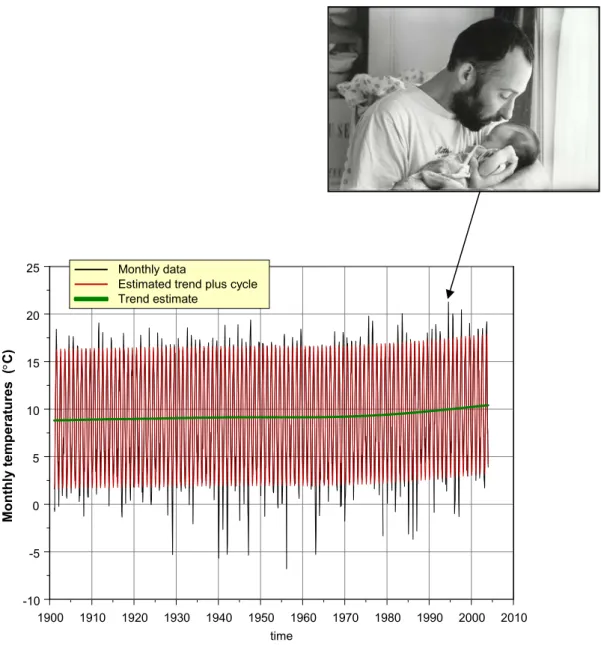
We have also estimated the annual cycle along with the long-term trend. This annual cycle has been based on monthly averaged data. Again, the estimation period is 1901-2003. The estimation results are given in Figure 4.2.
The coldest month in the record is that of February 1956, with a value of -6.8 ºC. The warmest month is that of July 1994 with a value of 21.3 ºC.
The trend is identical to the trend shown in Figure 4.1: − µJan 1901 = 8.8 [8.4, 9.2] ˚C
− µJuly 1950 = 9.2 [9.0, 9.3] ˚C
− µDec 2003 = 10.4 [10.1, 10.7] ˚C.
The structural time-series model allows the annual cycle to change over time. However, evaluation of the maximum likelihood function showed that the best model for the data is the one with a constant annual cycle. The annual cycle is given in Table 4.1.
We note that the residuals of the estimated model, shown in Figure 4.2 are slightly skewed and we estimated a comparative model using the transformation yt’ = ln (30-yt ). However
estimation results do not differ much. Therefore, we have chosen to present the simplest model, the one without transformation.
To show the impact of annual warming more clearly, we have redrawn the estimates from Figure 4.2. Figure 4.3 shows the annual cycles for five different years. We have also drawn a horizontal line at 5 °C. This line corresponds to the definition of ECA for the beginning and the end of the growing season.
The graph shows considerable growth in the length of the growing season over the 1950-2003 period. It starts ~16 days earlier in spring and ends ~14 days later in autumn. The graph also shows that an extra 1 or 2 degrees warming in the near future will have dramatic effects: the growing season will disappear completely (seen in the red), found completely above the 5 ºC threshold. One of the implications is that the winter hardening period for plants will disappear. A further discussion on the ecological impact of these shifts will be given in section 6.2.
Figure 4.2 Structural model with trend and cycle estimate for monthly averaged temperatures at the De Bilt station.
On the hottest day in the hottest month of the record (July 24, 1994) my son was born!
Table 4.1 Annual cycle in monthly temperatures, with an average of the 12 monthly temperatures at 0.0 K.
The uncertainty in these estimates is very small: 0.0016 K (2-σ limits). Jan. Feb. Mar. April May June July Aug
.
Sept. Oct. Nov. Dec. -7.19 K -6.65 K -4.21 K -1.22 K 3.15 K 5.72 K 7.49 K 7.20 K 4.65 K 0.80 K -3.58 K -6.15 K 1900 1910 1920 1930 1940 1950 1960 1970 1980 1990 2000 2010 time -10 -5 0 5 10 15 20 25 Monthly data
Estimated trend plus cycle Trend estimate Mo n th ly temp eratu res ( °C)
Figure 4.3 Annual temperature cycles for five different years.
The cycles are achieved by taking the estimated trend, µt, and adding the cycle, γt,
from Table 4.1. The blue horizontal line marks the threshold for initiating and ending the growing season. The orange and red cycles are added to the graph to show the impact of an extra 1 and 2 degrees warming in the near future. According to the inference made in section 8.1, these respective warming curves may become real around the years 2010 and 2020.
4.1.3 Are the results consistent with seasonal estimates?
Tang (2003) estimated trends for the individual seasons. He found that annual mean warming of 1.5 K over the 1901-2003 period as not uniformly distributed over the seasons:
− winter: µ2003 - µ1901 = 1.2 K − spring: µ2003 - µ1901 = 1.8 K − summer: µ2003 - µ1901 = 1.4 K − autumn: µ2003 - µ1901 = 1.2 K Jan uary February Marc h Ap ril May June July Augus t Se pt em be r Octo be r No vemb er De ce mb er 0.0 5.0 10.0 15.0 20.0 25.0 Ann u al cy cle ( °C)
initiation and ending of growing season
Trend plus cycle in 2003 plus 2 degrees Trend plus cycle in 2003 plus 1 degree Trend plus cycle in 2003
Trend plus cycle in 1950 Trend plus cycle in 1901
Clearly, maximum warming occurred in spring, and to a lesser extent in summer. These conclusions were also drawn by Van Oldenborgh and Van Ulden (2003) and KNMI (2003). In the last reference explanations are given for the unusual warming in winter and spring. Are these seasonal estimates contradictory to the results presented in Figure 4.2 and Table 4.1, where we conclude that warming is spread uniformly over the 12 months, and, consequently, uniformly over the seasons?
The discrepancy is easily understood if the uncertainty bands in seasonal warming are taken into account. These are as follows (Tang, 2003):
− annual: µ2003 - µ1901 = 1.5 ± 0.6 K
− winters: µ2003 - µ1901 = 1.2 ± 1.3 K
− spring: µ2003 - µ1901 = 1.8 ± 0.9 K
− summer: µ2003 - µ1901 = 1.4 ± 0.6 K
− autumn: µ2003 - µ1901 = 1.2 ± 0.7 K
Errors are 2-σ confidence limits. Due to the large inter-annual variability the limits appear to be very wide. As a consequence, the difference between winter warming and spring warming is far from statistically significant. And winter warming itself is barely significant.
The conclusion is that there is indeed a tendency for non-uniform warming across seasons. However, these differences are far from statistically significant.
4.2
Precipitation
4.2.1 Annual totals
How did annual precipitation sums evolve in the Netherlands? From the structural time-series model for De Bilt, shown in Figure 4.4, it can be seen that the minimum precipitation in the annual data falls in 1921 (407 mm) and the maximum in 1998 (1307 mm).
Trend statistics are:
• µ1906 = 768 [698, 838] mm
• µ2003 = 886 [816, 956] mm
• µ2003 - µ1906 = 118 [20, 216] mm
• µ2003 - µ2002 = 2.2 [-1.0, 5.4] mm
The results show a gradually increasing precipitation series with a small acceleration in this increase since 1970. The trend value in 2003 is statistically greater than all the trend values in the 1901-1970 (α = 0.05) period. This conclusion is consistent with that drawn by Bruin (2002) and KNMI (2003).
There is a significant increase in the annual amount of precipitation in the Netherlands. It has increased with 118 mm since 1901, i.e. an increase of 15% . Photo: C. Fetchmor.
Figure 4.4 Annual precipitation sums from 1906 to 2003 for De Bilt (black line), the estimated trend (green line) and the corresponding 95% confidence limits (dashed red lines). The lower panel shows the trend differences µ2003 – µt (mm). 1900 1910 1920 1930 1940 1950 1960 1970 1980 1990 2000 2010 400 600 800 1000 1200 1400 Annual data Trend estimate 95% confidence limits An nual p re ci p itation (mm) 1900 1910 1920 1930 1940 1950 1960 1970 1980 1990 2000 2010 Year -50 0 50 100 150 200 250 Trend difference 95% confidence limits Zero line µ2003 - µt (mm)
4.2.2 Annual cycle
We have also estimated the annual cycle along with the long-term trend to monthly precipitation sums. Because the residuals of the model directly estimated to the monthly data were skewed, we transformed the yt series to yt’ = log (15 + yt). The estimation results are
given in Figure 4.5. Minimum monthly precipitation occurred in September 1959, summed to 3 mm, and in February 1986, summed to 1 mm. Maximum precipitation (226 mm) occurred in August 1912 and in September 2001 (230 mm).
The trend estimates equal those shown in Figure 4.4: − µJan 1906 = 57 [52, 62] mm
− µJuly 1950 = 58 [55, 61] mm
− µDec 2003 = 65 [59, 71] mm.
The structural time-series model allows the annual cycle to change over time. However, evaluation of the maximum likelihood function showed the best model for the data to be the one with a constant annual cycle. The annual cycle is given in Table 4.2. Due to the logarithmic transformation the shape of the cycle component changes slightly over time. Figure 4.5 shows the annual cycle to be small relative to the trend values, varying between 3% and 16% relative to µt.
Figure 4.5 is also represented in Figure 4.6. The figure shows that all monthly precipitation sums have increased by approximately 7 mm since 1950.
Table 4.2 Annual cycle in monthly total precipitation for 1906-1950 (upper table) and for 2003 (lower table).
The average of the cycle is approximately 0 mm (due to model estimation on log-transformed data not being exactly 0 mm). The uncertainty in these estimates is negligible.
Jan. Feb. Mar. April May June July Aug Sept. Oct. Nov. Dec. 4 mm -15 mm -11 mm -13 mm -9 mm 2 mm 8 mm 11 mm 3 mm 4 mm 8 mm 11 mm Jan. Feb. Mar. April May June July Aug. Sept. Oct. Nov. Dec. 2 mm -17 mm -11 mm -15 mm -10 mm 4 mm 8 mm 12 mm 3 mm 6 mm 9 mm 13 mm
Figure 4.5 Structural time-series model with trend and cycle estimated for monthly precipitation sums at De Bilt. The model has been estimated using the transformation yt’ = ln( 15 + yt ).
Figure 4.6 Annual precipitation cycles for three different years.
1900 1910 1920 1930 1940 1950 1960 1970 1980 1990 2000 2010 Year 0 50 100 150 200 250
Estimated trend plus cycle Estimated trend Mo nt hly pr ec ip ita tio n ( m m ) Janu ary February Ma
rch April May June July
August Sept emberOctob er Nove mbe r Dece mber 0 20 40 60 80 100
Annual cycle for the year 1901 Annual cycle for the year 1950 Annual cycle for the year 2003
Mont hly p re ci pi ta tion (mm )
4.2.3 Are the results consistent with seasonal estimates?
Tang (2003) estimated trends for the individual seasons. He found that changes in annual precipitation totals over the 1906-2003 period not to be spread uniformly over the seasons (estimated on a slightly different precipitation series, based on daily pluviograph
measurements):
− winter: µ2003 - µ1906 = 20 mm
− spring: µ2003 - µ1906 = 28 mm
− summer: µ2003 - µ1906 = -20 mm
− autumn: µ2003 - µ1906 = 52 mm
As for the temperature estimates discussed in section 4.1.3 these seasonal estimates seem contradictory to the results presented in Figure 4.5 and Table 4.2, where we conclude that the annual increase in precipitation is spread uniformly over the 12 months, and, consequently, uniformly over the seasons.
Again, the discrepancy is easily understood if the uncertainty bands are taken into account. These are as follows (Tang, 2003):
− winter: µ2003 - µ1906 = 20 ± 40 mm
− spring: µ2003 - µ1906 = 28 ± 38 mm
− summer: µ2003 - µ1906 = -20 ± 50 mm
− autumn: µ2003 - µ1906 = 52 ± 50 mm
Errors are 2-σ confidence limits. Due to the large inter-annual variability the limits appear to be very wide. As a consequence, the difference between summer and autumn precipitation sums is not statistically significant. And only the autumn precipitation sum is just statistically significant - the other changes are not.
The conclusion is that there is indeed a tendency for non-uniform precipitation increases across seasons. However, these differences are far from statistically significant.
5.
Extreme weather conditions
5.1
Temperature
5.1.1 Absolute minimum temperatures
How did annual absolute minimum temperatures evolve in the Netherlands? In other words, what is the trend in the coldest moment in a year? Figure A.1 in Appendix A, upper panel, shows these data for main observatory De Bilt along with the average of the stations Den Helder, Groningen, De Bilt and Vlissingen. The graph shows good correspondence between the two series apart from the outlier at -25 ºC. It should be noted here that thermometers at all stations were lowered in height from 2.20 m to 1.50 m around 1961. Therefore, data before 1961 should be handled with some care (to correct for this inhomogeneity one should slightly lower temperatures before 1961, in the order of 0.1 K).
There is hope for one of the most popular outdoor winter sports in the Netherlands. The increase in temperature of the coldest moment of the year is not statistically significant
The structural time-series model for De Bilt is shown in Figure 5.1. Because of the skewness of minimum temperatures, the minimum temperatures were transformed into yt to
yt’= ln( -yt ).
Figure 5.1 Annual absolute minimum temperatures for De Bilt (black line), the estimated trend (green line) and the corresponding 95% confidence limits (dashed red lines).
Period is 1901-2003. Because of the skewness of minimum temperatures the original temperatures, yt, have been transformed to yt’= ln( -yt ). Estimated results have been
back-transformed in this panel. The lower panel shows the trend differences, µ2003 – µt
(ln(K)), based on the transformed model yt’.
1900 1910 1920 1930 1940 1950 1960 1970 1980 1990 2000 2010 -25.0 -20.0 -15.0 -10.0 -5.0
0.0 Annual minimum temperature Trend estimate 95% confidence limits Annu al absol u te min imum temp er atu res ( °C) 1900 1910 1920 1930 1940 1950 1960 1970 1980 1990 2000 2010 Year -0.4 -0.2 0.0 0.2 Trend difference 95% confidence limits Zero line Tren d di fference transformed d ata
The lowest annual minimum temperature is 24.8 °C (in 1942) and the maximum temperature is 3.9 °C (in 1990).
Trend statistics are:
• µ1901 = -11.4 [-13.0, -9.9] ºC
• µ2003 = -10.5 [-12.1, -9.2] ºC
• µ2003 - µ1901 = 0.9 [non significant] K
• µ2003 - µ2002 = 0.01 [non significant] K
The results show a slightly increasing temperature series. However, the trend in 2003 is not statistically larger than any of the trend values in the 1901-2002 period.
It is noted that the small inhomogeneity around 1961 would not change the result of a non-significant trend, as found above.