Experimental heat transfer measurements on supercritical R125 in a horizontal tube

(1)

supercritical R125 in a horizontal tube

Experimental heat transfer measurements on

Academic year 2019-2020

Master of Science in Electromechanical Engineering

Master's dissertation submitted in order to obtain the academic degree of

Counsellor: Jera Van Nieuwenhuyse

Supervisors: Prof. dr. ir. Michel De Paepe, Prof. dr. ir. Steven Lecompte

Student number: 01307537

(2)

(3)

supercritical R125 in a horizontal tube

Experimental heat transfer measurements on

Academic year 2019-2020

Master of Science in Electromechanical Engineering

Master's dissertation submitted in order to obtain the academic degree of

Counsellor: Jera Van Nieuwenhuyse

Supervisors: Prof. dr. ir. Michel De Paepe, Prof. dr. ir. Steven Lecompte

Student number: 01307537

(4)

Permission

The author gives permission to make this master dissertation available for consultation and to copy parts of this master dissertation for personal use.

In all cases of other use, the copyright terms have to be respected, in particular with regard to the obligation to state explicitly the source when quoting results from this master dissertation.

June 2020

(5)

Addendum

Due to the outbreak of the coronavirus in the beginning of 2020, safety measures were taken by Ghent University that restricted lab access. Fortunately, some measurements could still be performed. However, these are limited in number and parameter ranges.

(6)

Preface

Making this master thesis has proven to be quite a learnful experience and would not have been possible without the following people.

I would like to thank my supervisor Jera Van Nieuwenhuyse and promotors prof. Steven Lecompte and prof. Michel De Paepe for the opportunity and guidance. Thanks for answering my questions, reading and correcting this text, helping figuring out practical issues of the setup and performing measurements in particular.

Finally, I would like to thank my family and friends for all the support and necessary distractions during this year.

(7)

Experimental heat transfer measurements on supercritical R125

in a horizontal tube

Arthur De Meulemeester

Supervisors: prof. dr. ir. Michel De Paepe, prof. dr. ir. Steven Lecompte Counsellor: Jera Van Nieuwenhuyse

Master’s dissertation submitted in order to obtain the academic degree of Master of Science in Electromechanical Engineering

Departement of Electromechanical, Systems and Metal Engineering Chair: prof. dr. ir. Michel De Paepe

Faculty of Engineering and Architecture Ghent University

Academic year 2019–2020

Summary

This master thesis handles experimental heat transfer measurements on R125 at the supercritical state in a horizontal tube.

The introductory chapter explains why this research is needed and its main applications. Chapter two provides an overview of the different supercritical heat transfer phenomena. The influences of different parameters are discussed, as well as various supercritical heat transfer correlations found in literature.

The third chapter describes the test setup used to perform the measurements. An overview of all components and measurement equipment is given.

Chapter four describes the used data reduction method and corresponding uncertainty analysis.

Chapter five handles the results obtained from the performed measurements. First, the proposed combinations of parameters and their deviations are discussed. Second, the accuracy and repeatability is checked. Third, the influences of the operating parameters are investigated. Fourth, a first attempt at correlation development is done. Finally, the experimental results are compared to existing correlations found in literature.

The next chapter, chapter six, proposes adaptations to the existing setup to make buoyancy effects measurable and to obtain more accurate results.

Finally, the closing chapter provides a summary of the research and discusses future work.

(8)

MASTER THESIS 2019-2020 Research group Applied Thermodynamics and Heat Transfer Department of Electromechanical, Systems and Metal Engineering – Ghent University, UGent

EXPERIMENTAL HEAT TRANSFER MEASUREMENTS ON SUPERCRITICAL R125 IN A HORIZONTAL TUBE

Arthur De Meulemeester, Jera Van Nieuwenhuyse, Steven Lecompte and Michel De Paepe Department of Electromechanical, Systems and Metal Engineering

Ghent University

Sint-Pietersnieuwstraat 41, B9000 Gent, Belgium E-mail: arthur.demeulemeester@ugent.be

ABSTRACT

Utilisation of renewable and low-grade heat sources have a large potential to reduce greenhouse gas emissions, an ever growing concern. These energy sources include industrial waste heat, geothermal en-ergy, biomass combustion and solar energy. The or-ganic Rankine cycle (ORC), capable of converting low-temperature heat to useful work, has proved to be a suitable technology for this purpose. Its efficiency can be increased by operating at supercritical conditions, replacing the evaporator with a supercritical vapour generator. However, knowledge of the heat transfer behaviour of refrigerants at the supercritical state is limited. As only few heat transfer correlations are found in literature, more research is needed. In this pa-per, experimental measurements on supercritical heat transfer to supercritical R125 flowing in a horizontal tube were performed under various operating condi-tions. The setup consists of a counterflow tube-in-tube heat exchanger with a total length of 4 m. R125 flows in the inner tube, the heating fluid in the an-nulus. At 11 locations along this test section, bulk refrigerant temperatures are measured to determine the heat transfer coefficients. Influences of pressure, mass flux and heat flux were studied. Pressure lev-els varied between 1.04 and 1.11_·pc, mass fluxes

be-tween 320 and 600 kg/s/m2 _{and heat fluxes between}

8 and 21 kW/m2_{. The influences of these}

parame-ters agreed with conclusions found in literature: higher heat transfer coefficients were measured at lower pres-sures, higher mass fluxes and lower heat fluxes. How-ever, no peaks in heat transfer coefficients around the pseudocritical temperature as described in literature could be detected. Future work will adapt the mea-surement strategy to obtain more accurate results, broaden the operating range and test other low global warming potential (GWP) refrigerants.

NOMENCLATURE

cp [J/kg/K] Specific heat capacity

d [m] Inner tube diameter D [m] Outer tube diameter G [kg/s/m2_] _{Mass flux}

h [W/m2_/K] _{Convective heat transfer coefficient}

L [m] Test section length ˙

m [kg/s] Mass flow rate Nu [−] Nusselt number p [P a] Pressure Pr [−] Prandtl number

˙q [W/m2_] _{Heat flux}

˙

Q [W ] Heat transfer rate Re [−] Reynolds number T [◦_C] _Temperature Special characters µ [kg/m/s] Dynamic viscosity λ [W/m/K] Thermal conductivity ρ [kg/m3_] _Density Subscripts b Bulk c Critical hf Heating fluid i Inner in Inlet o Outer out Outlet pc Pseudocritical w Wall wf Working fluid INTRODUCTION

Supercritical operation of power and heat-to-heat cycles can have a positive influence on the cycle efficiencies compared to subcritical ones [1]. In the case of an ORC, the refrigerant in pressurized to a su-percritical pressure before heat addition, so the two-phase region is bypassed to get a so-called transcritical ORC. Designing the vapour generator of a transcriti-cal ORC requires accurate knowledge of the supercrit-ical heat transfer behaviour of the working fluid. To-day, many correlations can be found for water and/or

(9)

CO2. However, studies on supercritical heat

trans-fer on refrigerants are often not found. This gap in knowledge causes oversized heat exchanger designs and consequently higher costs. This research attempts to further close this gap by performing supercritical heat transfer measurements to supercritical R125 flowing in a horizontal tube.

SUPERCRITICAL HEAT TRANSFER

Heat transfer to supercritical fluids has been studied in the past. These studies showed that this type of heat transfer is heavily influenced by the rapid changes in thermophysical properties of the fluid. This leads to unusual heat transfer behaviour around the pseudo-critical temperature Tpc, defined as the temperature

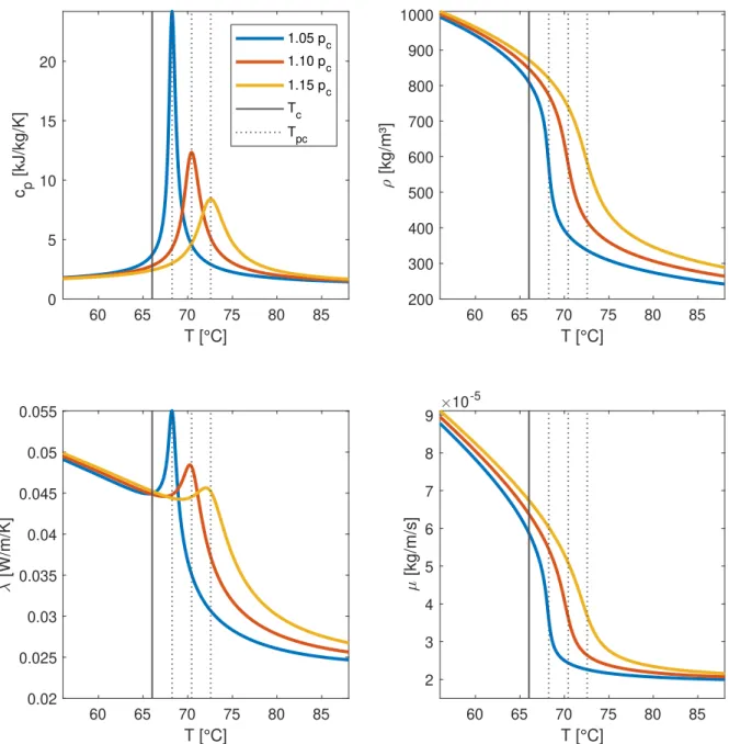
where the specific heat capacity has a peak for a cer-tain supercritical pressure [2]. Figure 1 shows varia-tions of the specific heat capacity cp, density ρ,

ther-mal conductivity λ and dynamic viscosity µ of R125 at a pressure 5% above pc. The vertical black lines

repre-sents the critical temperature Tc, the dotted lines Tpc.

Unlike at subcritical pressures, no discontinuities can be seen. 60 70 80 T [°C] 0 5 10 15 20 c p [kJ/kg/K] 60 70 80 T [°C] 200 400 600 800 [kg/m³] 60 70 80 T [°C] 0.02 0.03 0.04 0.05 [W/m/K] 60 70 80 T [°C] 2 4 6 8 [kg/m/s] 10-5

Figure 1: Thermophysical properties of R125 at su-percritical conditions

Influences on heat transfer behaviour

Supercritical fluids flowing in a horizontal tube are subject to buoyancy effects due to rapid density variations in the fluid, see Figure 1. Hotter and thus less dense fluid will rise to the top of the tube while heavier colder fluid will remain at the bottom. This natural convection leads to variable wall temperatures around the tube circumference and decreases the heat transfer coefficient at the top while the heat transfer coefficient at the bottom increases. This buoyancy

effect is present when low mass fluxes and/or high heat fluxes are used [3].

Apart from buoyancy effects, the pressure, mass flux and heat flux will influence the heat transfer behaviour. Higher convection coefficients are caused by decreased pressure, increased mass flux and decreased heat flux. In addition, the combination of thermophysical properties at and around Tpc causes

peaks in convection coefficients at these temperatures. Heat transfer correlations

Most supercritical heat transfer correlations found in literature are designed for water and/or CO2[4]. Some

results are found for refrigerants, such as R134a [5, 6], R125 [7] and R410a and R404a [8]. In these works, the influences of pressure, mass flux and heat flux were investigated.

TEST SETUP DESCRIPTION Setup overview

The test setup simulates the heat transfer of the vapour generator in a transcritical ORC. The pander, which is normally present in an ORC to ex-tract work, is replaced by an expansion valve. The setup was designed by Lazova et al. [7]. A schematic overview of the setup can be seen in Figure 2. It con-sists of three main loops: the heating, working fluid and cooling loop.

Preheater 2 Test section Preheater 1 Electric preheater Expansion valve Chiller Pump Condenser Thermal oil unit

Figure 2: Schematic overview of test setup The working fluid loop containing R125 is the main part of the setup. R125 (C2HF5) is an organic fluid

with a critical pressure of 3.6 MPa and a critical temperature of 66◦_{C, which makes it a suitable}

working fluid for low temperature waste heat recovery at the supercritical state. First, the working fluid is pressurized by the pump to a pressure above the critical pressure. The speed of the motor driving the pump is inverter controlled. After pressurization,

(10)

the refrigerant is preheated using two tube-in-tube preheaters and a 10 kW electric in-line preheater. By using these preheaters the refrigerant can be conditioned to the right temperature at the test section inlet. The use of the tube-in-tube preheaters is optional so either no, one or two preheaters are used. The electric preheater allows for a PID con-trolled temperature of the refrigerant at the test section inlet. After preheating, the refrigerant enters the test section. Next, the refrigerant flows through an electronically controlled expansion valve. After expansion, the refrigerant passes the condenser, which is a plate heat exchanger. The condenser is connected to the cooling loop which acts as a heat sink. The geometry and materials of the test section are shown in Table 1. It is a horizontal counterflow tube-in-tube heat exchanger with the refrigerant flowing in the inner tube and the heating fluid in the annulus. In the heating loop, Therminol ADX-10

Table 1: Test section specifications

Length 4 m

Inner tube Material Copper

λw 260 W/m/K

di 0.02477 m

do 0.02857 m

Outer tube Material Galvanised steel

Di 0.0530 m

Do 0.0603 m

thermal oil is used. After heating in the thermal oil unit it passes the test section and tube-in-tube preheaters. The thermal oil unit controls the oil tem-perature and has a heating capacity of 20 kW. The mass flow rate through the test section is controlled by a three way valve.

At the condenser, the refrigerant is cooled down by the cooling loop. It contains a mixture of wa-ter/glycol (70/30%) and is connected to a 900 l buffer vessel. This vessel is cooled by a 37 kW chiller unit located at the outside of the building. Just as in the heating loop, a three way valve allows for mass flow rate control through the condenser.

Test section measurement equipment

At the oil side of the test section, Pt100 tempera-ture sensors are placed at inlet and outlet. In be-tween, three K-type thermocouples are spaced evenly throughout the test section at distances of 1 m. Sim-ilarly, at the refrigerant side Pt100 sensors are placed at inlet and outlet. Between these, 11 T-type thermo-couples are spaced evenly at distances of 0.33 m. In addition, pressure transducers are placed at inlet and outlet. Figure 3 shows a schematic overview of the test section including all temperature measurements. Red arrows indicate the thermal oil, blue arrows the

refrigerant flow. During test measurements it became

Figure 3: Test section thermocouple placements clear that not all measurement equipment provided reliable results. The thermocouple measurements at the oil side of the test section proved to be unreliable. The opposite is true at the refrigerant side, where the Pt100 sensors did not function properly. In addition, four thermocouples at the refrigerant side of the test section could not be used. The measured temperatures by these thermocouples were too high, a possible planation being that they were not located at the ex-act tube centre, but closer to the tube wall. While the malfunctioning measurement equipment described above did influence the control strategy and the data reduction method, reliable measurements could still be performed.

DATA REDUCTION METHOD AND UN-CERTAINTY ANALYSIS

Data reduction method

Starting from the heat exchanger geometry and mea-sured data, the convection coefficients at the refriger-ant side can be determined. First, the heat transfer rate ˙Q and heat flux ˙qhf in the test section is

deter-mined at the oil side. ˙ Q = ˙mhf· cp,hf· ∆Thf (1) ˙qhf = ˙ Q π_{· d}o· L (2) As only oil temperatures at the inlet and outlet of the test section are known, the oil temperature profile is assumed to be linear. The consequence of this is the assumption of a constant heat flux over the test section. In addition, heat losses to the environment are neglected.

The outer wall temperature Tw,o can be found

as a function of the measured bulk oil temperature Thf,b, heat flux ˙qhf and oil side convection coefficient

hhf, determined using the Dittus-Boelter correlation

[9]. Tw,o= Thf,b− ˙qhf hhf (3) N uhf = hhf· (Di− do) λhf = 0.023_{· Re}0.8 hf · P r0.3hf (4)

In the next step, the inner wall temperature Tw,i is

(11)

drop over the inner tube wall. Tw,i= Tw,o− ˙ Q· ln(do/di) 2π_{· λ}w· L (5) Finally, the convection coefficient at the refrigerant side hwfand corresponding Nusselt number N uwf can

be calculated. ˙qwf = ˙ Q π_{· d}i· L (6) hwf = ˙qwf Tw,i− Twf,b (7) N uwf = hwf· di λwf (8)

Uncertainty analysis and accuracy of results Errors on the measured quantities and the used ther-mophysical properties in the data reduction method will propagate through the results. The calculation of these propagations is determined by the method described by Moffat [10]. Table 2 shows the needed accuracies. It is clear from Equation 1 that a higher Table 2: Accuracies of sensors and thermophysical properties

Thermocouples 0.1 K

Pt100 0.1 K

Pressure transducers 6000 Pa

Mass flow meters 1%

cp,hf 1 J/kg/K

µhf 0.00001 Pa·s

λhf 0.0001 W/m/K

λwf 3% [11]

heat flux will cause a larger temperature difference over the test section for both the heating and working fluid. Another consequence of this is an improved accuracy of the calculated convection coefficients. As

˙

mhf is fixed, a larger ∆Thf corresponds to a smaller

uncertainty of ˙Q. The error on the final results are mostly due to the uncertainty of ∆Thf and the

accuracy of the Dittus-Boelter correlation. The lat-ter is assumed constant under all operating conditions. It is important that the results found under cer-tain operating conditions are reproducible. Figure 4 shows three separate measurements performed under approximately equal operating conditions. First of all it is clear that obtaining the exact same heat flux is more difficult than obtaining the same pressure and mass flux. Second, it shows that the results are indeed reproducible, the deviations between the different measurements are much smaller than their error bars. Even though the measured datasets are limited in temperature range and accuracy, general trends can still be seen, which will be discussed in the next section.

66 68 70 72 74

Refrigerant bulk temperature [°C]

600 800 1000 1200 h [W/m 2 /K] p = 1.11 x p c, G = 327 kg/s/m 2_{, q = 19.2 kW/m}2 p = 1.11 x p c, G = 325 kg/s/m 2_{, q = 20.8 kW/m}2 p = 1.11 x p c, G = 325 kg/s/m 2_{, q = 20.8 kW/m}2

Figure 4: Repeatability check

EXPERIMENTAL RESULTS Operating conditions

Two pressure levels corresponding to 5 and 10% above the critical pressure pc were tested with pseudocritical

temperatures of 68.3 and 70.4◦C respectively. Heat fluxes of 10 and 20 kW/m2_{were chosen, corresponding}

to heat transfer rates of 3.11 and 6.23 kW. Four dif-ferent mass fluxes between 300 and 600 kg/s/m2 were investigated, corresponding to refrigerant mass flow rates between 0.145 and 0.289 kg/s. Combining these parameters results in 16 different operating conditions. The refrigerant pressure pwf is controlled by the

expansion valve position. Higher pressures are reached when it is closed more and vice versa. The re-frigerant mass flux Gwf is controlled by the rotational

speed of the pump. Higher mass fluxes are reached at increased rotational speeds and vice versa. The heat flux ˙qwf could not be controlled directly. For a given

pwf and Gwf, ˙qwf depends on the refrigerant inlet

temperature Twf,in, thermal oil inlet temperature

Thf,in and the thermal oil mass flow rate ˙mhf. From

Equation 4 it is clear that an increase in ˙mhf and

Thf,in result in a larger hhf and thus an increase in

heat flux. For this reason, ˙mhf was chosen to be

fixed at 2 kg/s during all measurements while Thf,in

was varied to reach the desired heat flux. Twf,in

was chosen such that the pseudocritical tempera-ture was reached around the middle of the test section. Reaching the exact proposed operating condi-tions was not possible. For the desired pressure of 1.05_{· p}c, pressures between 1.04· pc and 1.06· pc were

reached. Likewise, for the desired pressure of 1.10· pc,

(12)

Mass fluxes of 320, 430, 510 and 600 kg/s/m2 _were

obtained. Using the method described above to control ˙qwf, deviations from the setpoints are in the

order of 0.5 to 1 kW/m2_{. Apart from the proposed}

measurement conditions, some measurements were also performed with heat fluxes of about 16 to 18 kW/m2_.

The tube diameter, heat flux, mass flux and pressure will have effects on the results. As the tube dimen-sions do not change, the influence of the other three parameters can be studied. In the next section, one example is shown for each influence. In these graphs, the dotted vertical lines indicate the pseudocritical temperature of the dataset of the same colour. A consequence of the limited measurement accuracy is the overlap of all compared data. Nevertheless, general trends in the measured convection coefficients can still be observed. The error bars are not shown in the graphs for clarity reasons.

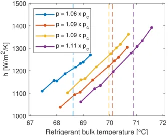
Influence of pressure

Figure 5 shows the measured convection coefficients as a function of the bulk refrigerant temperature for different pressures at the same mass and heat flux. As expected, an increase in pressure results in a de-crease in heat transfer coefficients. Due to the limited measurement accuracy, the two measurements for a pressure of 1.09· pc show varying results. Still, the

expected influence of the pressure holds.

67 68 69 70 71 72

1000 1100 1200 1300 1400 1500 h [W/m 2 /K] p = 1.06 x p_c p = 1.09 x p_c p = 1.09 x p_c p = 1.11 x p_c

Figure 5: Influence of pressure at Gwf=320 kg/s/m2

and ˙qwf=10 kW/m2

Comparisons of convection coefficients at other com-binations of mass and heat fluxes show similar results. In one case, the influence of the pressure level is not very clear. This is presumably caused by the limited accuracy of the setup.

Influence of mass flux

Figure 6 shows the measured convection coefficients as a function of the bulk refrigerant temperature for dif-ferent mass fluxes at the same pressure and heat flux. The results meet the expectation, a higher mass flux and thus a higher Reynolds number causes increased convection coefficients.

64 66 68 70 72

700 800 900 1000 1100 1200 1300 h [W/m 2 /K] G = 593 kg/s/m2 G = 506 kg/s/m2 G = 426 kg/s/m2 G = 327 kg/s/m2

Figure 6: Influence of mass flux at pwf=1.10 x pcand

˙qwf=20 kW/m2

In all other comparisons, large deviations in mass flux result in clear differences in convection coefficients. However, if the difference is smaller (comparison be-tween 600 and 510 kg/s/m2 _{for example), the}

differ-ence can be very small or zero. Again, this could be explained by the limited measurement accuracy. Influence of heat flux

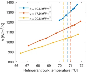
Figure 7 shows the measured convection coefficients as a function of the bulk refrigerant temperature for dif-ferent heat fluxes at the same pressure and mass flux. Also in this case the results are as expected, higher heat fluxes lead to decreased convection coefficients. In all other comparisons, heat fluxes of 10 kW/m2

clearly result in higher convection coefficients com-pared to 20 kW/m2_{. In some cases, no clear difference}

can be seen when comparing datasets of 17-18 and 20 kW/m2_{. Again, this could be explained by the limited}

measurement accuracy. Wilson plots

A first step to develop a new correlation can be made using the Wilson plot method [12]. Figure 8 shows all data points from the measurement matrix together with a linear fitting. Red dots represent the data for a heat flux of 20 kW/m2_{, blue dots for a heat flux}

of 10 kW/m2_. _{Note that only a limited range of}

Reynolds numbers is present in the dataset, ranging from about 130· 103_{to 630}_{· 10}3_{. Still, larger Reynolds}

(13)

66 67 68 69 70 71 72

800 900 1000 1100 1200 1300 1400 h [W/m 2 /K] q = 10.6 kW/m2 q = 17.9 kW/m2 q = 20.6 kW/m2

Figure 7: Influence of heat flux at pwf=1.10 x pc and

˙

Gwf=430 kg/s/m2

numbers correspond to higher Nusselt numbers gener-ally. The fitted curve for the whole dataset results in N ub= 10.186· Re0.329b . 5.1 5.2 5.3 5.4 5.5 5.6 5.7 5.8 log(Re) [-] 2 2.2 2.4 2.6 2.8 3 log(Nu) [-] q = 10 kW/m2: y = 0.286x + 1.293 all data: y = 0.329x + 1.008 q = 20 kW/m2: y = 0.316x + 1.013 q = 10 kW/m2: y = 0.286x + 1.293 all data: y = 0.329x + 1.008 q = 20 kW/m2: y = 0.316x + 1.013 q = 10 kW/m2: y = 0.286x + 1.293 all data: y = 0.329x + 1.008 q = 20 kW/m2: y = 0.316x + 1.013 q = 10 kW/m2: y = 0.286x + 1.293 all data: y = 0.329x + 1.008 q = 20 kW/m2: y = 0.316x + 1.013 q = 10 kW/m2: y = 0.286x + 1.293 all data: y = 0.329x + 1.008 q = 20 kW/m2: y = 0.316x + 1.013 q = 10 kW/m2: y = 0.286x + 1.293 all data: y = 0.329x + 1.008 q = 20 kW/m2: y = 0.316x + 1.013 q = 10 kW/m2: y = 0.286x + 1.293 all data: y = 0.329x + 1.008 q = 20 kW/m2: y = 0.316x + 1.013 q = 10 kW/m2: y = 0.286x + 1.293 all data: y = 0.329x + 1.008 q = 20 kW/m2: y = 0.316x + 1.013 q = 10 kW/m2: y = 0.286x + 1.293 all data: y = 0.329x + 1.008 q = 20 kW/m2: y = 0.316x + 1.013 q = 10 kW/m2: y = 0.286x + 1.293 all data: y = 0.329x + 1.008 q = 20 kW/m2: y = 0.316x + 1.013 q = 10 kW/m2: y = 0.286x + 1.293 all data: y = 0.329x + 1.008 q = 20 kW/m2: y = 0.316x + 1.013 q = 10 kW/m2: y = 0.286x + 1.293 all data: y = 0.329x + 1.008 q = 20 kW/m2: y = 0.316x + 1.013 q = 10 kW/m2: y = 0.286x + 1.293 all data: y = 0.329x + 1.008 q = 20 kW/m2: y = 0.316x + 1.013 q = 10 kW/m2: y = 0.286x + 1.293 all data: y = 0.329x + 1.008 q = 20 kW/m2: y = 0.316x + 1.013 q = 10 kW/m2: y = 0.286x + 1.293 all data: y = 0.329x + 1.008 q = 20 kW/m2: y = 0.316x + 1.013 q = 10 kW/m2: y = 0.286x + 1.293 all data: y = 0.329x + 1.008 q = 20 kW/m2: y = 0.316x + 1.013 q = 10 kW/m2: y = 0.286x + 1.293 all data: y = 0.329x + 1.008 q = 20 kW/m2: y = 0.316x + 1.013 q = 10 kW/m2: y = 0.286x + 1.293 all data: y = 0.329x + 1.008 q = 20 kW/m2: y = 0.316x + 1.013 q = 10 kW/m2: y = 0.286x + 1.293 all data: y = 0.329x + 1.008 q = 20 kW/m2: y = 0.316x + 1.013 q = 10 kW/m2: y = 0.286x + 1.293 all data: y = 0.329x + 1.008 q = 20 kW/m2: y = 0.316x + 1.013 q = 10 kW/m2: y = 0.286x + 1.293 all data: y = 0.329x + 1.008 q = 20 kW/m2: y = 0.316x + 1.013 q = 10 kW/m2: y = 0.286x + 1.293 all data: y = 0.329x + 1.008 q = 20 kW/m2: y = 0.316x + 1.013 q = 10 kW/m2: y = 0.286x + 1.293 all data: y = 0.329x + 1.008 q = 20 kW/m2: y = 0.316x + 1.013 q = 10 kW/m2: y = 0.286x + 1.293 all data: y = 0.329x + 1.008 q = 20 kW/m2: y = 0.316x + 1.013 q = 10 kW/m2: y = 0.286x + 1.293 all data: y = 0.329x + 1.008 q = 20 kW/m2: y = 0.316x + 1.013 q = 10 kW/m2: y = 0.286x + 1.293 all data: y = 0.329x + 1.008 q = 20 kW/m2: y = 0.316x + 1.013 q = 10 kW/m2: y = 0.286x + 1.293 all data: y = 0.329x + 1.008 q = 20 kW/m2: y = 0.316x + 1.013 q = 10 kW/m2: y = 0.286x + 1.293 all data: y = 0.329x + 1.008 q = 20 kW/m2: y = 0.316x + 1.013 q = 10 kW/m2: y = 0.286x + 1.293 all data: y = 0.329x + 1.008 q = 20 kW/m2: y = 0.316x + 1.013 q = 10 kW/m2: y = 0.286x + 1.293 all data: y = 0.329x + 1.008 q = 20 kW/m2: y = 0.316x + 1.013 q = 10 kW/m2: y = 0.286x + 1.293 all data: y = 0.329x + 1.008 q = 20 kW/m2: y = 0.316x + 1.013 q = 10 kW/m2: y = 0.286x + 1.293 all data: y = 0.329x + 1.008 q = 20 kW/m2: y = 0.316x + 1.013

Figure 8: Wilson plots

In addition, this dataset can be split up according to the heat flux. As explained above, increasing the heat flux results in lower convection coefficients. The fitted curves are almost parallel for this range of Reynolds number. This leads to the conclusion that the influ-ence of the heat flux on the obtained convection coef-ficients is more or less independent of the refrigerant Reynolds number. In addition, the fitted curve for all data in the measurement matrix lies between the red and blue curves as expected.

Heat transfer coefficient peaks

In all measurements, no peaks in heat transfer coeffi-cients were seen at or around the pseudocritical tem-perature. This is opposed to different results found in

literature. This is presumably caused by two factors. First, no wall temperature measurements are incorpo-rated in the measurement setup. Buoyancy effects are to be expected as the test section is placed horizontally, causing higher convection coefficients at the bottom of the tube. Because no variation in wall temperature is assumed in the data reduction, these effects could not be measured in any way. Second, ˙Q was assumed to be constant over the test section length because of the malfunctioning thermocouples at the thermal oil side. As ˙qhfand ˙Q are needed to determine the temperature

drops due to convection at the oil side and conduction through the inner tube wall, the resulting values for Tw,ido not vary much over the test section length and

presumably deviate from the actual inner wall tem-peratures. According to Equation 7, this heavily in-fluences the obtained values for hwf.

CONCLUSION AND FUTURE WORK

Measurements on supercritical R125 flowing in a horizontal tube were performed at pressures between 1.04· pc and 1.11· pc, refrigerant mass fluxes between

320 and 600 kg/s/m2 _{and heat fluxes between 9 and}

22 kW/m2_{. The influences of the pressure, mass flux}

and heat flux could be investigated. In general, lower pressures, higher mass fluxes and lower heat fluxes result in higher convection coefficients. These results agree with expected results found in literature. While the accuracy on the convection coefficients proved to be quite low, a first step to develop a new correlation could be done. Using the Wilson plot method, a linear trend could be seen for log(N ub)

as a function of log(Reb). Higher bulk Reynolds

numbers correspond to larger Nusselt numbers and thus larger convection coefficients. When the data was split up according to low and high heat flux, a clear difference could be seen. The lower heat flux resulted in approximately a fixed increase in log(N ub)

for the range of tested Reynolds numbers.

Future work includes broadening the bulk refrig-erant temperature, pressure, mass flux and heat flux ranges. In addition, the setup will be adapted such that wall temperature measurements are included. This leads to the detection of variable wall tem-peratures over the inner tube circumference due to buoyancy effects. In addition, this would greatly improve the accuracy on the obtained convection coefficients since the Dittus-Boelter correlation would not be needed in the data reduction. Finally, the setup can be adapted for testing other low GWP working fluids suitable for heat recovery applications at the supercritical state.

(14)

REFERENCES

[1] S. Lecompte, E. Ntavou, B. Tchanche, G. Kosmadakis, A. Pillai, D. Manolakos, and M. de Paepe, “Review of experimental research on supercritical and transcritical thermodynamic cycles designed for heat recovery application,” Applied Sciences, vol. 9, no. 12, pp. 1–26, 2019. [2] K. Yamagata, K. Nishikawa, S. Hasegawa, T.

Fu-jii, and S. Yoshia, “Forced convective heat trans-fer to supercritical water flowing in tubes,” In-ternational Journal of Heat and Mass Transfer, vol. 15, no. 12, pp. 2575–2593, 1972.

[3] S. Yu, H. Li, X. Lei, Y. Feng, Y. Zhang, H. He, and T. Wang, “Influence of buoyancy on heat transfer to water flowing in horizontal tubes un-der supercritical pressure,” Applied Thermal En-gineering, vol. 59, no. 1-2, pp. 380–388, 2013. [4] M. Bazargan, Forced convection heat transfer to

turbulent flow of supercritical water in a round horizontal tube. PhD thesis, 2001.

[5] C. R. Zhao and P. X. Jiang, “Experimental study of in-tube cooling heat transfer and pressure drop characteristics of R134a at supercritical pres-sures,” Experimental Thermal and Fluid Science, vol. 35, no. 7, pp. 1293–1303, 2011.

[6] R. Tian, D. Wang, Y. Zhang, Y. Ma, H. Li, and L. Shi, “Experimental study of the heat trans-fer characteristics of supercritical pressure R134a in a horizontal tube,” Experimental Thermal and Fluid Science, vol. 100, pp. 49–61, 2019.

[7] M. Lazova, A. Kaya, S. Lecompte, and M. De Paepe, “Presentation of a test-rig for heat trans-fer measurements of a fluid at supercritical state for organic Rankine cycle application,” in Pro-ceedings of the 16th International Heat Transfer Conference, pp. 8389–8396, 2018.

[8] S. Garimella, “Near-critical/supercritical heat transfer measurements of R-410a is small diam-eter tube,” tech. rep., Georgia Institute Of Tech-nology, 2008.

[9] F. Dittus and L. Boelter, “Heat Transfer in Au-tomobile Radiators of the Tubular Type,” Publi-cations in Engineering, University of California, Berkeley, vol. 2, no. 13, pp. 443–461, 1930. [10] R. J. Moffat, “Describing the uncertainties in

ex-perimental results,” Exex-perimental Thermal and Fluid Science, vol. 1, no. 1, pp. 3–17, 1988. [11] R. A. Perkins and M. L. Huber, “Measurement

and correlation of the thermal conductivity of pentafluoroethane (R125) from 190 K to 512 K at pressures to 70 MPa,” Journal of Chemical and Engineering Data, vol. 51, no. 3, pp. 898–904, 2006.

[12] J. Fern´andez-Seara, F. J. Uh´ıa, J. Sieres, and A. Campo, “Experimental apparatus for measur-ing heat transfer coefficients by the Wilson plot method,” European Journal of Physics, vol. 26, no. 3, 2005.

(15)

List of Figures

1.1 Ideal Rankine cycle layout with corresponding T-s diagram . . . 2

1.2 T-s diagram of the supercritical and transcritical ORC . . . 3

1.3 Temperature profiles of the subcritical and transcritical ORC . . . 4

1.4 T-s diagrams of wet, dry and isentropic fluids . . . 5

2.1 Variation of specific heat capacity, density, thermal conductivity and viscosity at supercritical conditions for R125 . . . 7

2.2 Buoyancy influence on wall temperatures . . . 8

2.3 Buoyancy influence on heat transfer coefficients . . . 9

2.4 Temperature profiles along radius by Wang et al. . . 10

2.5 Velocity profile of supercritical CO2 in a horizontal tube by Wang et al. . . 10

2.6 Wall temperatures as a function of bulk enthalpy for different heat fluxes . 11 2.7 Heat transfer coefficients as a function of bulk temperatures for different heat fluxes . . . 12

2.8 Wall temperatures as a function of bulk enthalpy for different mass fluxes . 13 2.9 Heat transfer coefficients as a function of bulk enthalpy for different mass fluxes . . . 13

2.10 Various DHT criteria versus experimental data . . . 14

2.11 Top, bottom and bulk temperatures measured by Bazargan et al. . . 14

2.12 Heat transfer coefficients measured by Bazargan et al. . . 15

2.13 Heat transfer coefficients measured by Zhao and Jiang . . . 19

2.14 Comparison of measured heat transfer coefficients and different correlations 20 2.15 Wall temperatures and heat transfer coefficients for different heat fluxes in a smooth and microfin tube by Wang et al. . . 21

2.16 Wall temperatures and heat transfer coefficients for different pressures in a smooth and microfin tube by Wang et al. . . 22

2.17 Effect of pressure and diameter on heat transfer coefficients for different mass fluxes by Garimella . . . 23

(19)

xix

2.18 Experimental Nusselt numbers as a function of bulk Reynolds number by

Garimella . . . 24

2.19 Heat transfer coefficient measurements by Lazova et al. . . 25

3.1 Schematic overview of test setup . . . 27

3.2 Test setup . . . 28

3.3 Thermocouple placement in test section . . . 31

3.4 Oil temperature measurements example . . . 33

3.5 Refrigerant temperature measurements example . . . 34

3.6 Positioning of Pt100 sensors and pressure transducers at refrigerant side . . 34

5.1 Accuracies of hwf and refrigerant temperature range for measurements at high Gwf and low ˙qwf . . . 43

5.2 Accuracies of hwf and refrigerant temperature range for measurements at low Gwf and high ˙qwf . . . 43

5.3 Example of repeatability check . . . 44

5.4 Influence of pressure at Gwf=320 kg/s/m2 and ˙qwf=10 kW/m2 . . . 45

5.5 Influence of mass flux at pwf=1.10·pc and ˙qwf=20 kW/m2 . . . 46

5.6 Influence of heat flux at pwf=1.10·pc and Gwf=430 kg/s/m2 . . . 46

5.7 Wilson plot method . . . 48

5.8 Wilson plots of experimental data with comparison between heat fluxes . . 49

6.1 Proposed wall temperature measurement locations . . . 53

6.2 Accuracy improvement of hwf for measurements at high Gwf and low ˙qwf . 54 6.3 Accuracy improvement of hwf for measurements at low Gwf and high ˙qwf . 54 B.1 Influence of pressure at Gwf=320 kg/s/m2 and ˙qwf=20 kW/m2 . . . 65

B.2 Influence of pressure at Gwf=430 kg/s/m2 and ˙qwf=18 kW/m2 . . . 66

B.4 Influence of pressure at G_wf=510 kg/s/m2 and ˙q_wf=20 kW/m2 . . . 66

B.6 Influence of mass flux at pwf=1.05·pc and ˙qwf=10 kW/m2 . . . 67

(20)

xx

B.12 Influence of heat flux at pwf=1.10·pc and Gwf=320 kg/s/m2 . . . 68

(21)

List of Tables

2.1 Overview of HTC influences . . . 16

3.1 Test section specifications . . . 29

3.2 Overview of sensor measurements . . . 32

3.3 Accuracies of measurement equipment . . . 32

4.1 Accuracies of thermophysical properties . . . 38

5.1 Proposed experimental matrix . . . 41

5.2 Comparison between experimental results and the correlation by Miropolski and Shitsman . . . 51

5.3 Comparison between experimental results and the correlation by Krasnoshchekov and Protopopov . . . 51

5.4 Comparison between experimental results and the correlation by Swenson et al. . . 51

5.5 Comparison between experimental results and the correlation by Jackson and Hall . . . 51

5.6 Comparison between experimental results and the correlation by Yu et al. . 52

6.1 Examples of working fluids with a critical pressure below 50 bar and a limited GWP and Tc . . . 55

C.1 Overview of performed measurements . . . 72

C.2 Results of data reduction . . . 73

(22)

Nomenclature

Abbreviations

DHT Deteriorated heat transfer

GWP Global warming potential

HTC Heat transfer coefficient

IHT Improved heat transfer

LMTD Logarithmic mean temperature difference

NHT Normal heat transfer

ODP Ozone depletion potential

ORC Organic Rankine cycle

Symbols

β Thermal expansion coefficient K−1

˙

m Mass flow rate kg/s

˙

Q Heat transfer rate W

˙ q Heat flux W/m2 λ Thermal conductivity W/(m_{· K)} µ Dynamic viscosity kg/(m_{· s)} ν Kinematic viscosity m2/s ρ Mass density kg/m3 A Surface area m2

cp Specific heat capacity J/(kg· K)

D Diameter outer tube m

d Diameter inner tube m

G Mass flux kg/(m2 _{· s)} Gr Grashof number ₋ h Convection coefficient W/(m2_{· K)} h Specific enthalpy J/kg L Length m N u Nusselt number ₋ xxii

(23)

xxiii p Pressure P a P r Prandtl number ₋ Re Reynolds number ₋ s Specific entropy J/(kg_{· K)} T Temperature K v Velocity m/s W Power W Subscripts b Bulk c Critical hf Heating fluid i Inner in Inlet o Outer out Outlet pc Pseudocritical w Wall wf Working fluid

(24)

Chapter 1 Introduction

One of the largest challenges facing the energy sector today is providing increasing amounts of energy while reducing its environmental impact. Finding sustainable ways to meet our energy demand is not only needed to lower greenhouse gas emissions and reduce global warming effects, but also because fossil fuels are exhaustible [1]. Up until now, large-scale electricity production is mostly done by combustion of fossil fuels such as gas, oil and coal or by nuclear power plants. Many power plants based on these fuels use a water/steam Rankine cycle, explained in Section 1.1. The main problem is that all of these sources (oil, gas, coal and nuclear) are non-renewable. On top of that, gas,

oil and coal based power plants emit large amounts of CO2 and other pollutants into the

atmosphere.

A different approach could be the use of other (renewable) heat sources such as solar and geothermal energy, in which heat is typically available at a lower temperature compared to conventional power plants [2]. The organic Rankine cycle (ORC), explained in section 1.2, has proven to be suitable technology for heat-to-power applications. For heat-to-heat systems, heat pumps are starting to replace classical gas boilers nowadays to provide heat to buildings. They are based on the vapour compression refrigeration cycle.

In practice, the cycles mentioned above have mostly evolved from subcritical to

supercritical operation [3]. Thermodynamic cycles operating under supercritical

conditions have proven to be a good way to increase efficiencies compared to subcritical cycles [4]. A fluid is at the supercritical state when its temperature and pressure are above its critical temperature and pressure, explained further in this chapter. Thermodynamic cycles of interest include heat-to-power (Rankine, Brayton) and heat-to-heat (heat pump) cycles. The importance for improved efficiencies is clear in heat-to-power cycles: for the same amount of work provided, less energy is needed as an input.

As is the case for the water/steam Rankine cycle, operation under supercritical conditions can benefit the efficiency of an ORC or heat pump cycle. Today, research is still needed to study supercritical heat transfer behaviour and its impact on the cycle components [4]. Knowledge of this heat transfer behaviour is beneficial for heat exchanger design used in these technologies as the lack of accurate correlations often lead to oversized heat exchangers.

At Ghent University, a transcritical ORC setup to determine supercritical heat transfer behaviour was built in the previous years. The evaporator of this setup is a horizontal

(25)

Chapter 1. Introduction 2

tube-in-tube counterflow heat exchanger and is rigged with measurement equipment to

determine local convection coefficients of the working fluid. The focus of this thesis

lies on the supercritical heat transfer behaviour at transcritical ORC conditions. In

the introductory chapter, the ORC is introduced. In the next chapter, an overview of supercritical heat transfer and the main goal of this thesis are given.

1.1 The water/steam Rankine cycle

To convert heat into useful work, the water/steam Rankine cycle can be used. The cycle consists of four main components and is depicted in Figure 1.1.

First, in an ideal cycle, saturated liquid is isentropically compressed to a higher pressure using a pump. Second, heat is added at a constant pressure in a boiler until the compressed liquid has become saturated or superheated vapour. Third, it is expanded isentropically to a lower pressure in an expander. This is where work is extracted. Finally, heat is rejected in the condenser at a constant pressure until the saturated liquid state is reached again, closing the cycle [3]. Figure 1.1 shows the ideal Rankine cycle, where in reality compression and expansion are not perfectly isentropic and pressure losses exist during evaporation and condensation.

Figure 1.1: Ideal Rankine cycle layout with corresponding T-s diagram [5]

1.2 The organic Rankine cycle

On the level of the cycle components, an ORC does not differ significantly from a classic water/steam Rankine cycle. The main difference lies in the working fluid and applications. Instead of water/steam, an organic fluid is used that is able to evaporate at lower temperatures, making them more suitable for converting heat from low-temperature heat sources into power. Such heat sources include industrial waste heat, geothermal heat, biomass combustion and solar heat [4].

(26)

1.2.1 ORC classification

Multiple different ORC architectures exist which can be classified into three categories depending on the pressures and temperatures used [4]: subcritical, transcritical and

supercritical. Important for this characterization are the critical temperature Tc and

critical pressure pc. The critical temperature is the highest temperature at which liquid

and vapour phases can coexist in equilibrium, the pressure at this so-called critical point is the critical pressure [3]. In a T-s diagram, this is the point where the saturated liquid and saturated vapour lines meet.

First, an ORC is called subcritical when both the evaporator and condenser pressures are below the critical pressure of the working fluid. This means that the cycle passes the two-phase region twice, during evaporation and condensation. The T-s diagram is identical to the one in Figure 1.1. Second, the transcritical ORC has an evaporation pressure that exceeds the critical pressure of the working fluid and a condensation pressure below the critical pressure. The result is that the two-phase region is avoided during evaporation so no discontinuity is present in the temperature profile during evaporation. Third, in the supercritical ORC, evaporation and condensation both take place at

supercritical pressures. The cycle never passes the two-phase region. In literature,

the term supercritical is also often used for a transcritical ORC [4]. In this work, the definitions as stated above will be followed. The typical T-s diagrams of the supercritical and transcritical ORC are shown in Figure 1.2.

Figure 1.2: T-s diagram of the supercritical (left) and transcritical (right) ORC [6]

1.2.2 The transcritical ORC

When using a heat source with a finite heat capacity, heat transfer will not take place at a constant heat source temperature. If the evaporation process of a subcritical and transcritical ORC are compared, a better temperature match is found for the transcritical cycle. The temperature profiles can be seen in Figure 1.3. In the transcritical case, no discontinuity in the temperature profile is seen during evaporation. This causes smaller temperature differences to exist in the evaporator, compared to the subcritical cycle. This can lower the irreversibilities in the heat exchanger, lower exergy destruction and improve the efficiency of the cycle because of these smaller temperature differences [7, 8]. This efficiency η is defined as the ratio of the net work extracted to the total heat input of the cycle: η = ˙ Wnet ˙ Qin = ˙ Wextr− ˙Wpump ˙ Qin (1.1)

(27)

Where ˙Qin is the heat added to the working fluid by the heat source, W˙extr is the

power extracted during expansion and ˙W_pump is the power consumed by the pump. The

theoretical maximum for this efficiency is given by the Carnot efficiency and only depends

on the temperatures TL and TH at which the heat is transferred:

ηmax = 1−

TL

T_H (1.2)

Where TL is the temperature of the cold source and TH the temperature of the heating

source. It is clear that this maximum efficiency will always be smaller than one and lowers

when the temperature difference between TL and TH decreases.

Figure 1.3: Temperature profiles of the subcritical (left) and transcritical (right) ORC [9]

1.3 Working fluid selection

When selecting the working fluid for a certain application, multiple factors should be taken into account [10–12]:

• General properties: Preferably a chemically stable, non-fouling and non-corrosive working fluid.

• Safety: Preferably a non-toxic and non-flammable working fluid.

• Saturation curve shape: Depending on the slope of the saturation curve (dT/ds) at the vapour side in the T-s diagram, a working fluid can be either dry, isentropic or wet. This is defined by the factor ξ = ds/dT, the inverse of that slope. ξ>0 holds for a dry fluid, ξ=0 holds for an isentropic fluid and ξ<0 holds for a wet fluid. The difference can be seen in Figure 1.4. This naming is easily explained: when the working fluid is a saturated vapour, a wet working fluid will expand to the two-phase region. Likewise a dry working fluid will expand to the superheated vapour region and an isentropic working fluid to a saturated vapour again. In general, dry and isentropic fluids are preferred since no superheating is required to avoid liquid droplets forming in the turbine or other expansion device.

• ODP and GWP: The ozone depletion potential (ODP) is the amount of degradation a refrigerant causes to the ozone layer, compared to R-11 (CCl₃F). Since the international Montreal protocol was signed in 1987, refrigerants with a ODP over

(28)

zero were phased out and are forbidden nowadays. The global warming potential (GWP) indicates how large the greenhouse effect is of a refrigerant, compared to CO2. It is preferably low.

• Critical parameters: The critical temperature Tc should not exceed the

temperature of the heat source in a transcritical cycle. The critical pressure p_c is

preferably not too high, since higher pressures lead to potential dangerous situations and higher pumping power, lowering the net work extracted.

Figure 1.4: T-s diagrams of wet, dry and isentropic fluids [7]

For the case of a transcritical ORC, the critical parameters of the working fluid should

match the heat source. This implies a critical temperature below the heat source

temperature and a limited critical pressure. In addition, low GWP refrigerants are

preferred to limit its environmental impact. As in any thermodynamic cycle, the general and safety properties should be satisfied as well.

In the vapour generator of a transcritical ORC, heat is added to the working fluid supercritically. The next chapter gives an overview of the knowledge on this type of heat transfer. The main focus lies on heat transfer occurring in horizontal tubes because the test setup, described in the third chapter, is of this type and is prone to certain specific phenomena.

(29)

Chapter 2 An overview of supercritical heat

transfer

Heat transfer to supercritical fluids has been studied in the past. These studies show that this heat transfer is heavily influenced by the rapid changes in thermophysical properties of the fluid. This leads to unusual heat transfer behaviour around the pseudocritical

temperature T_pc, defined as the temperature where the specific heat capacity has a peak

for a certain supercritical pressure [13]. Three expressions are used for describing the heat transfer phenomena at supercritical conditions: normal heat transfer (NHT), improved heat transfer (IHT) and deteriorated heat transfer (DHT) [14]. In the case of NHT, heat transfer coefficients are similar to subcritical convective heat transfer coefficients, determined by the single-phase Dittus-Boelter type correlations. IHT provides higher values compared to NHT and is associated with lower (local) wall temperatures. For DHT, lower heat transfer coefficients compared to NHT are present, resulting in higher (local) wall temperatures.

2.1 Thermophysical properties at supercritical

conditions

In Figure 2.1 variations of the specific heat capacity cp, density ρ, thermal conductivity

λ and dynamic viscosity µ can be seen for R125, which has a critical temperature of

66◦C (black vertical line) and a critical pressure of 36 bar [15]. For these properties,

three isobars are shown corresponding to pressures of 5, 10 and 15% above the critical pressure. Figure 2.1 was made using the CoolProp library [15]. It is immediately clear that these properties do not show discontinuities at supercritical pressures as opposed to the discontinuities present at the phase transitions at subcritical conditions.

For the specific heat capacity, a peak is visible for each pressure at their pseudocritical

temperatures (black vertical dotted lines). It is also clear that Tpc increases with the

pressure and the peak in specific heat capacity decreases with the pressure. For the density, thermal conductivity and viscosity a sudden decrease is visible at the pseudocritical temperature. For higher pressures, these effects become less distinct. In general, the thermophysical properties of the fluid will change most rapidly around the pseudocritical

(30)

Chapter 2. An overview of supercritical heat transfer 7

temperature and the fluid will be more liquid-like at temperatures lower than Tpc and

more gas-like when its temperature exceeds T_pc.

60 65 70 75 80 85 T [°C] 0 5 10 15 20 c p [kJ/kg/K] 1.05 p c 1.10 p_c 1.15 p_c T_c T_pc 60 65 70 75 80 85 T [°C] 200 300 400 500 600 700 800 900 1000 [kg/m³] 60 65 70 75 80 85 T [°C] 0.02 0.025 0.03 0.035 0.04 0.045 0.05 0.055 [W/m/K] 60 65 70 75 80 85 T [°C] 2 3 4 5 6 7 8 9 [kg/m/s] 10-5

Figure 2.1: Variation of specific heat capacity, density, thermal conductivity and viscosity at supercritical conditions for R125

2.2 Influences on heat transfer behaviour

Often disagreements between existing heat transfer correlations and experimental data of supercritical fluids are found. This is caused by the rapid variation of thermophysical properties in the supercritical region [16]. In general, the heat transfer behaviour at supercritical conditions is influenced by the pressure, mass flux, heat flux and tube

diameter. Depending on these variables, buoyancy effects may take place which can

(31)

2.2.1 Buoyancy effects

Supercritical fluids flowing in a horizontal tube are subject to buoyancy effects due to rapid density variations in the fluid, see Figure 2.1. Hotter and thus less dense fluid will rise to the top of the tube while heavier colder fluid will remain at the bottom. This natural convection leads to variable wall temperatures around the tube circumference and decreases the heat transfer coefficient at the top while the heat transfer coefficient at the bottom increases. This buoyancy effect is present when low mass fluxes and/or high heat fluxes are used [16, 17]. Research on this effect in horizontal tubes was first done in the 1960s by Krasyakova et al. [18] and Shitsman [19] on supercritical water who observed these temperature differences.

More recently, Yu et al. [17] performed experimental research on the buoyancy effect on supercritical water in horizontal tubes. Inner tube diameters were 26 and 43 mm, pressure

25 MPa, mass flux 300 to 1000 kg/(m2s) and heat fluxes up to 400 kW/m2. In Figures 2.2

and 2.3 wall temperatures and heat transfer coefficients can be seen as a function of the

bulk enthalpy for a mass flux of 600 kg/(m2s) and a heat flux of 300 kW/m2. It is clear

that the wall temperatures at the top are higher than at the bottom of the tube, with a

temperature difference of up to 80◦C. However, at higher bulk enthalpies (and thus higher

bulk temperatures, so further away from the pseudocritical temperature) this temperature difference seems to disappear. This is because the thermophysical properties do not vary rapidly any more in this region, so buoyancy effects driven by density differences will be less significant. When looking at the heat transfer coefficients, it is clear that IHT takes place near and before the pseudocritical point for the bottom surface of the tube while heat transfer at the top remains more constant, but has lower values. Also, it can be seen that for high enthalpies the heat transfer coefficients are almost equal which is caused by the nearly equal wall temperatures as described above.

(32)

Figure 2.3: Buoyancy influence on heat transfer coefficients [17]

Wang et al. [20] have performed numerical simulations for supercritical CO2 in large

horizontal tube diameters. An inlet temperature of 15.4◦C, pressure of 7.59 MPa and

heat flux of 15.1 kW/m2 was used as input. The variation of temperatures can be seen in

Figure 2.4. It is clear that a radial temperature profile is present, with strong variations near the tube walls. Further downstream in the tube, at higher bulk temperatures, the temperature difference between top and bottom increases. This agrees with the results of Yu et al. described above, since the shown temperatures are below the pseudocritical temperature of 32◦C in this simulation.

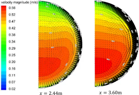
The velocity profile along two sections can be seen in Figure 2.5. Clearly, natural

convection takes place in the tube as seen by the circulation near the sides of the tube. This causes a layered structure that is more distinct further in the tube. Fluid velocities appear to be higher at the lower half of the tube, which in this work is explained by a thicker boundary layer at the top of the tube. This thicker boundary layer is caused by the secondary flow that takes the near-wall fluid upward, causing the low-momentum flow to accumulate near the top of the tube [20].

(33)

Figure 2.4: Temperature profiles along radius by Wang et al. [20]

Figure 2.5: Velocity profile of supercritical CO₂ in a horizontal tube by Wang et al. [20]

In general, the buoyancy effect can have a large influence on wall temperatures and heat transfer coefficients. Different criteria were developed in the past to determine whether buoyancy effects will be present [21]. A widely used criterion developed by Jackson and

Hall [22] stated that the value of Gr/Re2 (also called the Richardson number) could

be used to evaluate the buoyancy effects in supercritical flows [17]. Re is the Reynolds number of the fluid and Gr is the Grashof number, defined for tubular flow as:

Re = v· D

ν (2.1)

Gr = g· β · (Tw− Tb)· D

3

(34)

With v the velocity of the fluid, D the inner diameter of the tube, ν the kinematic viscosity, β the thermal expansion coefficient and g the gravitational acceleration. So, the Grashof number is a measure for the ratio of buoyancy to viscous forces. Jackson and Hall stated that if Gr/Re2.7 < 10−5 the buoyancy effects are negligible for vertical flows. Zhang et al. [23] numerically investigated heat transfer to supercritical water in horizontal circular tubes with an inner diameter of 7.5 mm and found this criterion to be fairly accurate, even though it was developed for vertical flows. However, the results of Bazargan et al. [16] disagreed with this criterion for supercritical water flowing in a horizontal round tube with an inner diameter of 6.3 mm. They found the criterion of Petukhov and Polyakov [24], which uses alternative definitions for the Grashof number, to be a better predictor for the onset of buoyancy effects. So it can be concluded that, up until now, no single criterion is capable of accurately predicting whether buoyancy effects will emerge.

2.2.2 Influence of heat flux

Yamagata et al. [13] experimentally investigated the influence of the heat flux for heat transfer to supercritical water in horizontal and vertical tubes. In Figures 2.6 and 2.7 wall temperatures and heat transfer coefficients can be seen for the horizontal tubes case.

Heat fluxes of 233, 465, 698 and 930 kW/m2 were tested at a pressure of 245 bar, mass

flux of 1260 and 1830 kg/(m2s) and tube diameter of 7.5 mm. For the two lowest heat

fluxes, virtually no temperature difference can be seen between top and bottom of the tube. However, for the highest two heat fluxes temperature differences can be clearly seen which seem to increase with the heat flux. For the heat transfer coefficients, peaks around the pseudocritical temperature can be seen again. This peak occurs at a bulk

temperature slightly below Tpc while the corresponding wall temperature is higher than

Tpc. The maximum value of the heat transfer coefficients increases with lower heat fluxes.

These results indicate that buoyancy effects are more pronounced at higher heat fluxes.

(35)

Figure 2.7: Heat transfer coefficients as a function of bulk temperatures for different heat fluxes [13]

2.2.3 Influence of mass flux

The influence of mass flux was also studied in the research of Yu et al. [17], which was on water flowing in a horizontal tube. In Figures 2.8 and 2.9 wall temperatures and heat

transfer coefficients can be seen. A pressure of 25 MPa and a heat flux of 200 kW/m2 was

used, while the mass flux was set to 300 and 600 kg/(m2s). It is clear that for a lower mass flux a greater temperature difference is present between the top and bottom of the tube. At a mass flux of 600 kg/(m2s), only very little temperature differences exist between top and bottom. This leads to the conclusion that buoyancy effects are less dominant when using larger mass fluxes. When looking at the heat transfer coefficients, it is clear that for both heat fluxes IHT is visible at the bottom of the tube. However, the ratio in heat transfer coefficients between top and bottom is smaller for higher mass fluxes. Due to a higher mass flux, velocities will be higher and so the flow becomes more turbulent, leading to higher forced convective heat transfer. So it can be concluded that higher mass fluxes improve heat transfer both at top and bottom.

(36)

Figure 2.8: Wall temperatures as a function of bulk enthalpy for different mass fluxes [17]

Figure 2.9: Heat transfer coefficients as a function of bulk enthalpy for different mass fluxes [17]

Different criteria for determining the onset of deteriorated heat transfer were proposed in the past, based on a critical value for the heat flux as a function of the mass flux [21]. Figure 2.10 shows some examples compared to experimental data from different working fluids under different operating conditions. For the data is this figure, correlations for predicting onset of DHT based on the heat transfer properties of water are good predictors for supercritical heat transfer to water only. They all overpredict the experimental values

for CO2 significantly. The opposite holds true for correlations based on CO2, which tend

to underestimate empirical data for supercritical water flow. This leads to the conclusion that these available criteria for one working fluid cannot be directly applied for any other working fluid.

(37)

Figure 2.10: Various DHT criteria versus experimental data [21]

2.2.4 Influence of tube diameter

Bazargan et al. [16] also performed research on supercritical water in horizontal tubes

with pressures of 23 to 27 MPa, heat fluxes up to 310 kW/m2, mass fluxes ranging from

330 to 1230 kg/(m2s) and an inner tube diameter of 6.3 mm. They found similar results

as Yu et al. [17] (who performed experiments with inner tube diameters of 26 and 43 mm), which can be seen in Figures 2.11 and 2.12. The heat transfer coefficients are again highest at the bottom side around the pseudocritical temperature, so IHT is visible at the bottom while DHT is present at the top. Also, these temperature differences between top and bottom disappear at higher bulk enthalpies/temperatures.

(38)

Figure 2.12: Heat transfer coefficients measured by Bazargan et al. [16]

For a pressure of 24.4 MPa, a mass flux of 340 kg/(m2s) and a heat flux of 297 kW/m2,

temperature differences between top and bottom are only 30◦C. This is much lower than

the differences in Figure 2.2. When considering the similar testing conditions (except for the mass flux, which is lower in this case), this leads to the conclusion that the buoyancy effect is more effective in larger tube diameters. If this would not be the case, higher temperature differences would be observed in the research of Bazargan et al. since the mass flux is lower. However, the opposite is true.

Research by Tian et al. [25] investigated the effects of tube size on the heat transfer to supercritical R134a in ORC applications for diameters of 10.3 and 16 mm. It was

concluded that for small ratios of the heat flux to the mass flux ˙q/G, the tube diameter

hardly influences the wall temperatures and heat transfer coefficients. However, when ˙q/G

has higher values a larger tube diameter leads to larger temperature differences between top and bottom of the tube. This leads to the conclusion that larger tube diameters are

more susceptible to buoyancy effects, given that the value of ˙q/G is high enough. The

reason for this ˙q/G factor can be explained by the influence of heat and mass flux as

described above. When ˙q is large or G is small (and thus ˙q/G is large), larger buoyancy

effects are observed and vice versa.

2.2.5 Overview of influences

Provided all the information above, buoyancy effects become more dominant at low mass fluxes, high heat fluxes and large tube diameters for heat transfer to supercritical fluids

in horizontal tubes. When no significant buoyancy effects are observed, only forced

convection takes place. Otherwise, both forced and natural convection are present [21, 26]. An overview of the different influences is given in Table 2.1.

When buoyancy effects are negligible, increased heat transfer coefficients around Tpc are

due to the favourable combination of thermophysical properties such as the peak in specific heat capacity. As these properties show less strong variations for higher pressures, these effects become less strong at supercritical pressures further away from pc.

(39)

have a large influence on the heat transfer coefficients. In this case, heat transfer behaviour

is much more complex. For higher values of ˙q/G, differences in temperature and heat

transfer coefficients between top and bottom of the tube can be seen. This leads to DHT at the top and IHT at the bottom. When using high heat fluxes, heat transfer coefficients tend to increase as the mass flux increases. At lower heat fluxes, increased mass fluxes do not always provide better heat transfer behaviour. Smaller tube diameters are less susceptible to buoyancy effects than larger diameter tubes. Comparing different experimental results on the influence of pressure can lead to contradictory results.

Table 2.1: Overview of HTC influences

tube mass and heat flux pressure buoyancy effects

small HTC increases with G and decreases with

˙ q.

IHT at and around Tpc,

peaks becomes smaller for larger pressures. NHT away from Tpc.

Not present, negligible or small.

large HTC differences

observed between top and bottom, difference bepending on value of ˙q/G.

Still IHT at and around T_pc

but contradictory results. However, HTC peaks seem to also decrease for higher pressures mostly.

Heavily influence T_w and HTC differences over circumference. DHT at top of tube and IHT at bottom.

2.3 Heat transfer correlations

In the previous century, many forced convection heat transfer correlations were developed. Most empirical correlations for supercritical heat transfer were developed with water,

CO2 or helium as a fluid [14]. Many are variations on the Dittus-Boelter or Gnielinski

correlations [27–29].

The Dittus-Boelter correlation [30] was developed in 1930 and expresses the bulk Nusselt number as a function of the bulk Reynolds number and bulk Prandtl number:

N u_b = 0.023_{· Re}0.8_b _{· P r}n_b (2.3)

Where n=0.4 when the flow is heated and 0.3 when cooled. It was developed for

single-phase subcritical heat transfer and is supposed to be valid in the range 0.6 _{≤ P r}b ≤ 160,

Reb ≥ 104 and L/D≥ 10.

The correlation proposed by Gnielinski [31] in 1976 also depends on the bulk Reynolds

and bulk Prandtl number and is supposed to be valid in the range 104 _{≤ Re}_b _{≤ 5 · 10}6

and 0.5_{≤ P r}b ≤ 2000: N ub = (f /8)(Reb− 1000)P rb 1 + 12.7(f /8)0.5_{(P r}2/3 b − 1) (2.4) f = (0.79_{· ln(Re}_b)_{− 1.64)}−2 (2.5)

Experimental heat transfer measurements on supercritical R125 in a horizontal tube

supercritical R125 in a horizontal tube

Experimental heat transfer measurements on

supercritical R125 in a horizontal tube

Experimental heat transfer measurements on

Permission

Addendum

Preface

Experimental heat transfer measurements on supercritical R125

in a horizontal tube

Contents

List of Figures

List of Tables

Nomenclature

Chapter 1

Introduction

1.1

The water/steam Rankine cycle

1.2

The organic Rankine cycle

1.2.1

ORC classification

1.2.2

The transcritical ORC

1.3

Working fluid selection

Chapter 2

An overview of supercritical heat

transfer

2.1

Thermophysical properties at supercritical

conditions

2.2

Influences on heat transfer behaviour

2.2.1

Buoyancy effects

2.2.2

Influence of heat flux

2.2.3

Influence of mass flux

2.2.4

Influence of tube diameter

2.2.5

Overview of influences

2.3

Heat transfer correlations