Validating SimpleBox-Computed Steady-State Concentration Ratios

The research defined in this report has been performed by order and for the account of the Directorate-General of the Environment, Directorate of Chemicals, Safety and Radiation, as part of the project 607220, Risk assessment of metals and organic substances.

National Institute of Public Health and the Environment (RIVM), P.O. Box 1, 3720 BA Bilthoven, The Netherlands Tel: +31 - 30 - 274 38 75, Fax: +31 - 30 - 274 44 01

Validating SimpleBox-Computed Steady-state Concentration Ratios

J Bakker, LJ Brandes, HA den Hollander, D van de Meent, J Struijs

A

The SimpleBox procedure for testing the coherence of environmental quality objectives was critically examined by a Committee of the Dutch Health Council in 1995. The result was a recommendation by the Committee to test the validity of this specific application of

SimpleBox. The multi-media model SimpleBox version 2.0 was chosen as the most suitable model for use in the procedure to test the coherence of independently derived environmental quality objectives. Environmental concentrations of five substances, tetrachloroethylene, lindane, benzo[a]pyrene, fluoranthene and chrysene, were compared to predicted

concentration. More specifically, the monitoring data were used to derive concentration ratios for adjacent compartments; these were then compared to modelled steady-state concentration ratios, taking uncertainties in the model input parameters into account. From the results calculated concentration ratios were, in general, found not to deviate much more than a factor of 10 from the “observed” data. The discrepancy between the computed and “observed” ratios of concentrations in the air and soil compartments were much larger, exceeding a factor of 30.

A

The authors want to acknowledge Marc van der Meij of the research department of the province Noord-Holland, Leen Vermeulen of the province Zeeland for providing air quality data and Peter Hoogeveen of the National Institute of Inland Water Management (RIZA) who provided the water quality data of the DONAR-data base. The authors also want to thank the following people from the RIVM: Paul van der Poel and Bart Wesselink of the Laboratory for Waste Products and Emissions, Hans Eerens, Henk Bloem, Arien Stolk and Ed Buijsman of the Laboratory for Air Research, Peter van Puijenbroek and Coert Dagelet of the Laboratory for Water and Drinking-water Research and Hans van Grinsven of the Laboratory for Soil and Groundwater Research for their help.

C

SUMMARY ...7

SAMENVATTING...9

1. PROBLEM DEFINITION...11

1.1 BACKGROUND...11

1.2 NEED FOR VALIDATION OF SIMPLEBOX...12

1.3 GOAL...12

1.4 APPROACH...12

2. APPROACH TO MODEL VALIDATION...15

2.1 INTRODUCTION...15

2.2 DATA COLLECTION...15

2.3 MODELLING...16

2.4 TESTING METHODS FOR VALIDITY...16

2.5 CRITERIA FOR VALIDITY...18

3. OBSERVED ENVIRONMENTAL CONCENTRATIONS ...21

3.1 INTRODUCTION...21

3.2 LITERATURE SEARCH...21

3.3 JAPANESE DATA...22

3.4 AIR AND RAINWATER QUALITY MONITORING...22

3.5 WATER DATA...26

3.6 SOIL QUALITY DATA...29

3.7 SUMMARY...30

4. MODELLING...33

4.1 INTRODUCTION...33

4.2 MONTE CARLO SIMULATIONS...33

4.3 VARIABILITY AND UNCERTAINTY...33

4.4 MODEL SETTINGS FOR THE NETHERLANDS...34

4.5 CHEMICAL COMPOUND PROPERTIES...37

4.6 EMISSIONS...41

5. COMPARISON OF COMPUTED AND OBSERVED DATA ...47

5.1 INTRODUCTION...47

5.2 COMPUTED STEADY-STATE CONCENTRATIONS AND CONCENTRATION RATIOS...47

5.3 MONITORED COMPARED TO COMPUTED CONCENTRATIONS...49

5.4 OBSERVED COMPARED TO COMPUTED CONCENTRATION RATIOS...55

5.5 DERIVING COHERENCE CRITERIA...60

6. DISCUSSION...63

6.1 DATA...63

6.2 REQUIRED ACCURACY OF SSCRS FOR COHERENCE TESTING...63

6.3 STUDIED CHEMICALS...63

6.4 SOIL COMPARTMENTS...64

REFERENCES...69 APPENDIX I MAILING LIST ...77 APPENDIX II RESULTS OF THE LITERATURE SEARCH, CONCENTRATIONS OUTSIDE THE NETHERLANDS ...79 APPENDIX III OBSERVED CONCENTRATIONS OF PESTICIDES AND PCBS ...81 APPENDIX IV ESTIMATING STATISTICAL PARAMETERS FROM LIMITED DATA SETS ...85 APPENDIX V CHARACTERISTICS OF THE DISTRIBUTION OF OH-RADICAL

CONCENTRATIONS ...87 APPENDIX VI FREQUENCY DISTRIBUTIONS OF OBSERVED AND COMPUTED

CONCENTRATIONS...89 APPENDIX VII SCORES OF COMPUTED CONCENTRATIONS ON THE FACTOR 3, 10 AND 30 CRITERIA, ARE THE CRITERIA FULFILLED?...95 APPENDIX VIII FREQUENCY DISTRIBUTIONS OF OBSERVED AND COMPUTED

CONCENTRATION RATIOS...97 APPENDIX IX SCORES OF COMPUTED CONCENTRATION RATIOS ON THE FACTOR 3, 10 AND 30 CRITERIA, ARE THE CRITERIA MET? ...103 APPENDIX X PROBABILITY OF COMPUTED CRS FALLING WITHIN PREDEFINED

S

The Dutch Health Council identified model validation as a pre-requisite for applying models for regulatory purposes. Validation of multi-media models for estimating environmental fate was recommended by a SETAC Taskforce on the Application of Multi-Media Fate Models to Regulatory Decision-Making. This report documents the evaluation of the validity of the multi-media fate model, SimpleBox, version 2.0, with respect to its specific use in testing the coherence of independently derived environmental quality objectives. The objective of the evaluation was to test whether the model could predict steady-state intermediate

concentration ratios well enough for the purpose of coherence testing. Testing the validity of the underlying mechanistic assumptions in the model was considered to be beyond the scope of this project.

Predicted steady-state concentration ratios (SSCRs) were compared with measured environmental concentration ratios (MECRs). SimpleBox calculations of SSCRs require information on emission ratios, chemical properties and environmental settings. Monte Carlo sampling of input distributions takes the uncertainty of the SSCRs into account. Useful information, both on emission ratios and environmental concentrations, was either scarce or difficult to obtain. Chemicals, measured in air in the Netherlands, were generally not

measured or detected in water or soil. Concentration data from outside the Netherlands, e.g. the Great Lakes in Canada, were only available from the literature and resulted in a small set of air and water concentrations measured over a long period of time in different geographic areas. These data were therefore not particularly useful for validation. It also had to be considered that for modelling concentrations outside the Netherlands, a lot of region-specific environmental information would be needed that might be difficult to obtain.

Nevertheless, measured environmental concentrations in The Netherlands of five substances, lindane, tetrachloroethylene, fluoranthene, chrysene and benzo[a]pyrene, were used to

calculate water concentration ratios, and water sediment, water-suspended-matter and air-soil concentration ratios. These “measured” ratios were compared to the modelled

concentration ratios. Concentration ratios for air and water were, generally speaking, not found to deviate by more than a factor of 10. For water-sediment and water-suspended matter concentration ratios, the computed ratio of only benzo[a]pyrene was found to differ by just more than a factor of 3. Only for the air-soil concentration ratios large differences were observed, and then generally more than a factor of 30.

The uncertainties in the “measured” and calculated concentration ratios have about the same magnitude. Uncertainties in Environmental Quality Objectives are also about the same so there is no direct need to reduce uncertainties in predicted concentration ratios. There is also no reason to reject the application of SimpleBox in the procedure of testing the coherence of independently derived environmental quality objectives, at least, as long as there is no scientific alternative.

Comparison of modelled and observed concentration ratios indicates that the degree of certainty with which the predicted ratios fall within a chosen uncertainty interval, obviously tends to be higher using wider intervals. Certainty levels of the related uncertainty factors, i.e. 3, 10, 30 and 100, come to about 20%, 50%, 70% and 80%, respectively.

S

In dit rapport komt de validatie van het verspreidingsmodel SimpleBox 2.0 aan de orde. Bij de validatie is er met name gekeken naar een specifieke toepassing van het model, namelijk het toetsen van de ‘coherentie’ van onafhankelijk van elkaar afgeleide

milieukwaliteitsdoelstellingen. Het doel van dit rapport is om na te gaan of het model de verhoudingen van steady-state concentraties in aan elkaar grenzende compartimenten voldoende goed voorspelt voor het aantonen van inconsistenties in de onafhankelijk van elkaar afgeleide milieukwaliteitsdoelstellingen.

Dit naar aanleiding van het advies van de Nederlandse Gezondheidsraad waarin zij heeft aangegeven dat validatie een eerste vereiste is voor een model dat wordt toegepast in beleidsontwikkeling. Tevens adviseerde de gezondheidsraad een wetenschappelijke update van het model, inclusief gevoeligheids- en onzekerheidsanalyse. De SETAC taakgroep voor het toepassen van multi-media verspreidingsmodellen bij het ontwikkelen van

beleidsvoorschriften gaf eveneens een aanbeveling voor het valideren van verspreidingsmodellen.

De onzekerheid in de door het model voorspelde concentratieverhoudingen wordt onderzocht door het vergelijken van de voorspelde ratios met de verhouding van de in het milieu gemeten concentraties in aan elkaar grenzende compartimenten. Daartoe is informatie benodigd over zowel fysisch-chemische eigenschappen, emissies als omgevingsvariabelen. Met behulp van de Monte Carlo techniek wordt de onzekerheid in de invoer parameters doorberekend naar de modeluitvoer, de steady-state concentratieverhoudingen.

De hoeveelheid bruikbare informatie was vrij beperkt met betrekking tot zowel gemeten concentraties als emissies. Het komt vaak voor dat chemische stoffen die in de lucht worden gemeten niet worden aangetroffen of worden gemeten in het oppervlaktewater of in de bodem. Buitenlandse meetgegevens, zoals aangetroffen in de openbare literatuur kwamen vaak niet overeen in plaats en tijd. Voor regios buiten Nederland geldt tevens dat het verkrijgen van representatieve omgevingsvariabelen lastig kan zijn.

Voor een vijftal stoffen zijn de meetgegevens gebruikt om concentratieratios te berekenen. Het betreft: lindaan, tetrachlooretheen, fluorantheen, chryseen en benzo[a]pyreen. Deze zogenaamde ‘gemeten’ concetratieverhoudingen zijn vergeleken met de door het model SimpleBox berekende concentratieverhoudingen. De concentratieratios voor lucht-water verschillen meestal niet meer dan een faktor tien met de berekende ratios. Voor de concentratieverhoudingen van water-sediment en water-gesuspendeerd materiaal is het verschil voor slechts één stof meer dan een factor drie. Grote verschillen worden

waargenomen voor de verhouding tussen de concentraties in lucht (aerosolen/regenwater) en de bodem. Het verschil is meer dan een factor dertig.

De onzekerheid in de ‘gemeten’ en de gemodelleerde ratios is ongeveer even groot, en vergelijkbaar met de onzekerheid in de afgeleide milieukwaliteitsdoelstellingen. Daarom is het niet direct noodzakelijk om de onzekerheden in de modeluitkomsten te reduceren. Er is eveneens geen directe aanleiding om het model SimpleBox af te wijzen met betrekking tot het gebruik bij het afleiden van een coherente set van milieukwaliteitsdoelstellingen, waarbij moet worden opgemerkt dat een goed wetenschappelijk alternatief niet voorhanden is. Vergelijking van gemodelleerde en ‘gemeten’ ratios geeft aan dat de mate van zekerheid waarmee voorspelde ratios binnen een vooraf vastgestelde onzekerheidsmarge vallen, groter wordt naarmate grotere onzekerheidsmarges worden gebruikt. Deze mate van zekerheid is berekend voor verschillende onzekerheidsmarges en bedraagt voor de onzekerheidsfactoren 3, 10, 30 en 100 respectievelijk 30%, 50%, 70% en 80%.

1. P

D

SimpleBox (Van de Meent, 1993 and Brandes et al., 1996) is a multi-media environmental fate model. Models of this so-called Mackay-type are used and have been proposed for use in various regulatory frameworks (Cowan et al., 1995). In The Netherlands, SimpleBox has been used:

1. to predict steady-state intermedia concentration ratios for the purpose of harmonisation of environmental quality objectives (Health Council of The Netherlands, 1995);

2. to predict concentrations in the regional environment for the purpose of evaluation of chemicals (Van der Poel, 1997a).

Harmonisation of Environmental quality objectives

Within the research program ‘Setting Integrated Environmental Quality Objectives for Water, Soil and Air’ (INS-project), The Netherlands Directorate-General of the Environment (DGM) has started to derive harmonised or ‘coherent’ sets of environmental quality objectives. Maximum permissible concentrations (MPCs) in the environment are derived on the basis of the estimated 5th percentile of the distribution of NOECs. MPC-values are derived

independently for air (human toxicity data), water (aquatic ecotoxicity data), sediment

(sediment toxicity data), and soil (terrestrial ecotoxicity data). These sets of MPC-values may not be coherent in the sense that maintaining the environmental concentration in a given compartment exceeds the MPC derived for another compartment. Van de Meent and De Bruijn (1995) have proposed to use the steady-state intermedia concentration ratios (SSCR), as computed by SimpleBox, as a test for coherence of independently derived MPC-values. This SSCR procedure has been applied to derive harmonised environmental quality

objectives for a number of volatile organic chemicals (Van de Plassche and Bockting, 1993). In the past, the same modelling procedure has been used for computing critical concentrations in air, starting from MPC-values for soil (Van de Meent, 1995). The SSCR-procedure has been critically reviewed by a Committee of the Health Council of The Netherlands (Health Council of The Netherlands, 1995). The Health Council recommended that validation of SimpleBox is urgently needed. The Committee advised amongst others to validate the model as a whole as well as individual process descriptions.

Substances and Products Evaluation

The SimpleBox model has found application as a regional distribution model in the Uniform System for Evaluation of Substances (USES) (RIVM, VROM, WVC, 1994; Van der Poel, 1997a; EC, 1996). In this application, Predicted Environmental Concentrations (PEC) in air, water, sediment and soil at a regional spatial scale (The Netherlands) are computed on the basis of (predicted) emission rates. In the computation, the regional concentrations are computed, taking the continental concentrations as a ‘background’ (Van der Poel, 1997a). This application has drawn attention outside The Netherlands.

In Denmark, research has been carried out to evaluate the possibilities for use of SimpleBox in typical Danish settings, and to adapt the model to these specific needs (Fredenslund et al., 1995; Severinsen et al., 1996). The regional modelling part of USES has been applied to Life Cycle Analysis, for evaluating the impact of toxic substances emitted during the ‘cradle-to-grave sequence’ of products (Guinée et al., 1996). For this purpose, the model was set to European proportions as much as the USES framework allowed. The European Commission finished a European System for the Evaluation of Substances (EUSES) in 1997, taking the Dutch USES model as a starting point (EC, 1996; Jager et al., 1997).

1.2 Need for validation of SimpleBox

Until recently, multi-media fate models have primarily been used as research tools, to gain insight into the possible importance of intermedia transfer mechanisms, and to improve understanding of the importance of properties of chemicals in this respect. Hardly any serious attempt has been made so far to test the validity of this type of model as a tool for predicting concentrations or concentration ratios. Van de Meent and De Bruijn (1995) characterised the multi-media modelling concept as ‘non-validated’, and suggested at the same time to apply the concept, in absence of alternatives. While the usefulness of multi-media models in regulatory decision making is clear, the need for validation of this model type is even more evident.

Model validation was recommended by a SETAC Taskforce on Application of Multi-Media Fate Models to Regulatory Decision-Making (Cowan et al., 1995). The Health Council of The Netherlands identified model validation as a prerequisite for application of the model in regulatory practice (Health Council of The Netherlands, 1995).

1.3 Goal

The goal of the research described in this report was to evaluate the validity of the multi-media fate model SimpleBox with respect to its specific use in the procedure of testing the coherence of independently derived environmental quality objectives. The subject of this report is to validate the model as a whole: how well does the model describe the

environmental concentration ratios of specific chemicals in The Netherlands?

1.4 Approach

Scope of the validation

Focusing on the specific use for testing coherence of environmental quality objectives, has a number of implications:

With respect to the model output to be validated, the study is primarily restricted to quotients of pairs of steady-state concentrations at the regional spatial scale: the air-water, air-soil and water-sediment concentration ratios.

In line with this, first priority is given to validating the model as a whole; validation of individual process descriptions has a lower priority.

With respect to the model input, the study is restricted to situations in which the quantitative knowledge of ratios of emissions to the different environmental compartments is defined; knowledge of absolute rates of emission is not required because the SimpleBox model is a so-called linear model, the output (concentration ratios) is linearly dependent on the input

(emission ratios).

With respect to the chemicals, the study focuses on the chemicals for which integrated environmental quality objectives are being set in the INS-project: the typical micropollutants supposed to have toxic effects on humans and ecosystems. No particular set of chemicals has been identified a priori for this study. The model claims to be applicable to all chemicals, provided that the necessary model input in terms of partition coefficients is available. Therefore, in principle, validity needs to be tested for all chemicals.

With respect to the system, the study focuses on environmental situations that can be interpreted as representative for typical Dutch circumstances.

Validity

Criteria for accepting or rejecting the model validity are to be found in the level of certainty that is required for the proposed application of the model result. In this case: the possible decision to adjust an environmental quality objective if it is concluded that the derived Maximum Permissible Concentrations (MPCs) for two compartments are incoherent. In the proposed procedure, MPCs are called incoherent if the computed Steady-State Concentration Ratio exceeds the ratio of the independently derived MPCs by more than a factor of 10. The Health Council has recommended to base this judgement on actual uncertainties, rather than on this implicitly perceived uncertainty factor of 10. In this light, model calculations of SSCRs are considered valid if the uncertainty as it appears from comparison of computed and observed data is small enough to yield practically useful criteria for coherence of MPCs. The validation study is done with the SimpleBox version 2.0.

Uncertainty in model output

Taking the recommendations made by the Health Council and others into consideration, the assumptions made in SimpleBox -the possible sources of uncertainty and error- are reviewed, and prior to this study an uncertainty analysis was carried out. The methods and results of this uncertainty analysis are given in Etienne et al. (1997). In this study we have taken the

uncertainty in the model output into account by Monte Carlo sampling of input distributions. The result is a distribution of the steady-state air/water- and air/soil etc., concentration ratios.

Model

The original version (Figure 1.2) of the multimedia fate model SimpleBox is revised as a starting point for this validation study. A technical description of this version of SimpleBox (Figure 1.1) can be found in Brandes et al. (1996).

In the new version of SimpleBox the environment is modelled as a regional scale nested in continental and global scales. The regional and continental scale represent a densely populated Western European region and the whole of the European Union, respectively.

ARCTIC ZONE MODERATE ZONE TROPIC ZONE

GLOBAL SCALE CONTINENTAL SCALE

REGIONAL SCALE

Figure 1.1: Geographic scales in SimpleBox 2.0 (Brandes et al., 1996)

The spatial scales include homogeneous environmental compartments: air, freshwater and seawater compartments, sediments, three soil types and vegetation on natural and

agriculturally used soil. The global scale is divided in three zones: a moderate, arctic and tropic zone. Each zone consists of an air, seawater, sediment and soil compartment.

Figure 1.2: Six compartments (air, water, sediment three different soil types) in SimpleBox 1.0 (Van de Meent, 1993).

In SimpleBox 2.0, four compartments (marine water and sediment and vegetation on natural and agricultural soil) have been added (Brandes et al., 1996)

The model requires information on chemical properties and emission rates and calculates the distribution of the chemical between the environmental compartments. This study

concentrates on the regional scale, the model defaults are modified to represent the typical Dutch settings.

AIR

W ATER

SED

SOIL 1 SOIL 2 SOIL 3

GROUNDW ATER AIR

W ATER

SED

SOIL 1 SOIL 2 SOIL 3

2. A

Computed steady-state concentration ratios were compared with observed concentration ratios. Concentration data were obtained from the literature, databases of monitoring networks and by consultation of experts. An additional monitoring program was started for phthalates. However, this monitoring program is not a part of this project and the validation results are separately reported by Struijs (2002). It was anticipated that measured

concentrations in The Netherlands would be available for a limited number of well-known chemicals only, and that this selection of chemicals might not be as representative for the chemicals of the INS-list as one would like. Simultaneously measured concentration data for air, water, sediment and soil at the same locations in The Netherlands were expected to be exceptional. Data obtained from measurements outside The Netherlands are considered to be potentially useful in this validation project too (Japan, Denmark, Great Lakes in North America). For these data, the SimpleBox model definitions must be adjusted to represent the environmental situations for which the measurements were obtained.

2.2 Data collection

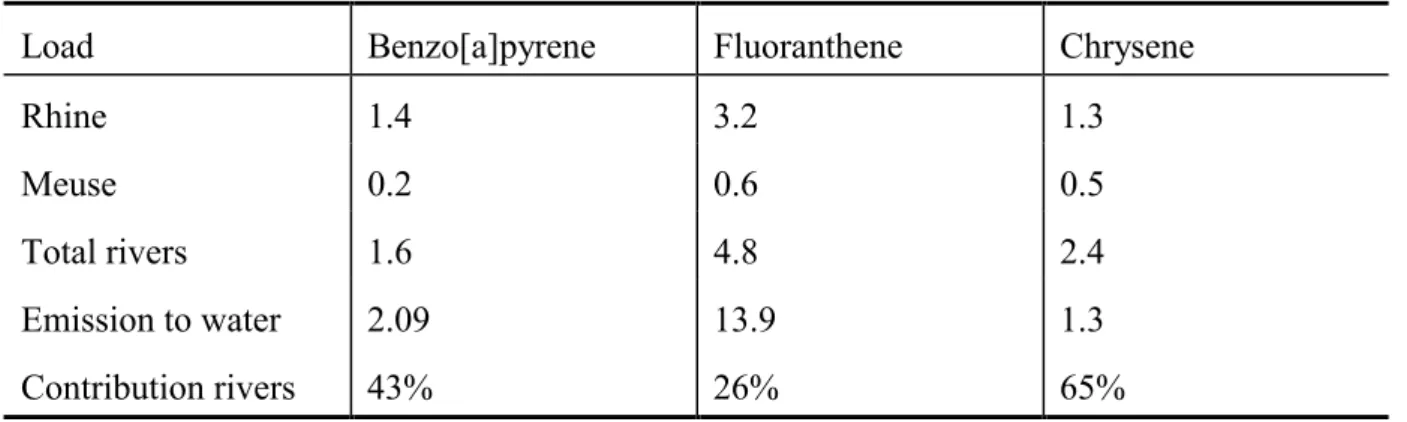
Four sorts of data are needed:

• loadings: amounts of a chemical that enter the system to be modelled (‘import’ with air and water, emissions to air, water and soil) and their probability distributions. Only relative amounts (percentage of total loadings) are needed because the model is linear in the emissions and the resulting concentrations and only relative statements on

concentrations are to be validated. But loadings are not exactly known and therefore the uncertainty has been accounted for.

• environmental descriptors: if the validity test is done for environmental settings other than the model default settings (The Netherlands), the characteristic parameters for that specific environmental situation are needed.

• concentrations: preferably concentrations in air, water, sediment and soil, measured at the same location, and at the same time, but concessions may be inevitable in case of lack of data.

• properties: physical and chemical properties, to be used as input to the model (partition coefficients, degradation rate constants) and their probability distributions.

Emission and concentration data are the most difficult categories. A selection of

representative, ‘INS-like’, chemicals was made on the basis of apparent data availability. Obvious candidates for selection were chemicals that have been addressed in other, similar model studies and for which monitoring data and fate parameters are known to be available.

Van de Meent and De Bruijn (1995) used benzene, 1,4-dichlorobenzene, 1,1,1,-trichloroethane, dichlorophenol, atrazine, benzo[a]pyrene and lead, to illustrate the

harmonization procedure. Mackay and others (1985,1992) have published model test results with benzene, chlorobenzene, 1,2,3-trichlorobenzene, hexachlorobenzene, and p-cresol. Devillers et al., and Bintein and Devillers used isobutylene (1995), lindane (1996a) and atrazine (1996b) to test the ChemFrance model. Verbruggen et al. (1997) used DDT, PCBs, DEHP and lead to test their global fate model. We have carried out a literature search for concentration data in air, water, sediment and soil, measured at the same regions and times. Two sorts of difficulties were foreseen: unstructured data plentifulness and data scarcity. To solve these problems, a scoping search was done first for DEHP and PCBs, using easily accessible open literature. Data was collected from the public literature and by actively searching for additional sources of data.

2.3 Modelling

For all suitable data sets, the output distributions of the SSCRs were calculated with SimpleBox 2.0 after parameterisation of the model for the type of environment from which the data originate. Considering the uncertainties in model inputs, probability distributions of compound specific and non-compound specific input parameters (environmental parameters) are required for the output distribution of the SSCRs. These resulting uncertainties in the model output refer to the assumption of well-mixed compartments and space- and time-averaged concentrations. The output distributions were obtained from Monte Carlo simulations.

2.4 Testing methods for validity

There are several statistical methods, which may be useful for assessing the performance of model output (Boekhold et al., 1993):

1. Graphical methods 2. Factor-of-f-approach

3. Comparison of confidence intervals 4. Comparison of mean values

5. Comparison of variances

Graphical methods

Graphs can be very useful in showing trends and distributions. Because the validation results must be readily interpretable by users of the system, the choice for a graphical representation seems to be more appropriate, instead of presenting the results of a validation study with statistical methods (Jager, 1995).

Graphical methods may include comparison of observed and predicted values, comparison of ranges of observed and predicted values and comparison of (cumulative) distribution

functions of observed and predicted values.

Factor-of-f-approach

The Factor-of-f-approach is a method for testing whether model predictions fall within a prescribed factor of true values. Parrish and Smith (1990) describe the method of the Factor-of-f-approach.

Comparison of confidence intervals

By means of Monte Carlo simulation techniques one can obtain the characteristics of the probability density functions (PDF) of the output, which result from the uncertainties in the input parameters. If the shape and characteristics of the PDF of model output parameters is known, a particular confidence interval can be constructed. This confidence interval is dependent on the desired level of significance α. Comparison of the confidence intervals resulting from the model simulations with the confidence intervals of the measurements is described by Parrish and Smith (1990).

Comparison of mean values

Statistical tests such as a Student’s t-test can be used to test whether model predictions are the same as true values. But, in practice predicted values will rarely equal the true values, thus the hypothesis will be rejected routinely. For the application of environmental models in

management, the hypothesis of equality and this testing approach may be too stringent (Parrish and Smith, 1990).

An approach to design a statistically meaningful test is to test the hypothesis that the

difference between predicted and measured mean values does not exceed a predefined value. This value can be chosen such, that a certain amount of imprecision is allowed (Boekhold et al., 1993). Further statistical details can be found in Mood et al. (1974).

Comparison of variances

For comparison of variances multiple measurements and multiple model outputs must be known. This can be achieved by using Monte Carlo simulations. The Kolmogorov-Smirnov procedure tests for goodness of fit of model predictions to the distribution of measurements (D’Agostino and Stephens, 1986).

2.5 Criteria for validity1

Model predictions of SSCRs are valid if the uncertainty, as it appears from comparison of computed and observed data, is small enough to be useful in the practice of coherence testing. Coherence criteria:

Maximum Permissible Concentrations (MPCs) are called incoherent if the computed steady-state concentration ratio exceeds the ratio of the independently derived maximum permissible concentrations by more then a factor of 10 (Van de Meent and De Bruijn, 1995). Example: if a certain chemical is emitted to air, and MPCs of 1 mg/m3 and 1 µg/l, for air and water, respectively, are derived, and the SimpleBox calculation predicts an air-water steady-state concentration ratio of 90 l/m3, then the ratio of MPCs, Maximum Permissible Concentration Ratio (MPCR), exceeds the ratio of Steady-State Concentrations (SSCs), SSCR, by more than a factor 10:

MPCR MPC

MPC

g m

g l l m SSCR

air water air water air water − − − − = =10 = ≥ ⋅ 10 1000 10 3 3 6 3 / / /

In this example, the model predicts that if the concentration in air would be maintained at the level of MPCair, the concentration in water would exceed the MPCwater by more than a factor of 10: C MPC SSCR g m l m g l MPC water air air water water = = = > ⋅ − − 10 90 111 10 3 3 3 / / . µ /

As pointed out by the Health Council, there is no scientific rationale for the use of a factor of 10 as a threshold criteria for incoherence, other than perhaps that this is the perceived

uncertainty of the predicted SSCR. No formal probabilistic basis has been proposed for coherence criteria. A useful probabilistic criterion for example could be the 90% confidence level of the quotient of MPCR and SSCR. A set of MPCs could be called incoherent, if the quotient MPCR and SSCR differs from the value 1 with more than 90% certainty. If the MPCR/SSCR quotient has a lognormal distribution with an uncertainty factor of ten2, this probabilistic criterion would match with the factor-of-10 criteria.

90 . 0 10 10 > þ ý ü î í ì_{− < <} SSCR MPCR P

1 _{In case of validating SimpleBox by means of comparing calculated SSCR with Measured Environmental}

Concentration Ratios (MECR); MPCR can be replaced by MECR and MPC by the environmental concentration (C) through out this paragraph.

Application of the criteria requires quantitative assessment of the distributions (uncertainties) of both the SSCR and the MPCR. There are three situations possible:

1. The relative uncertainty in MPCR is much greater than the relative uncertainty in SSCR. In this case, the uncertainty in SSCR is negligible, and the practical usefulness of the

coherence test is determined by the uncertainty in MPCR only.

2. The relative uncertainty in SSCR is much greater than the relative uncertainty in MPCR. In this case, the practical usefulness of the coherence test is fully determined by the

uncertainty in SSCR.

3. The relative uncertainties have similar magnitudes. In this case both uncertainties contribute to the practical usefulness of the coherence criteria.

Clearly, probabilistic criteria for validity of the model calculations of SSCR can only be set if the required level of confidence (acceptable level of certainty) for coherence test is defined, and the uncertainty in MPCR is known.

As a guideline, a priory criteria for testing model predictions against field data of the SETAC-Workshop (Cowan et al., 1995) can be used. The perceived accuracy factors are based on the assumption that the emission rate is known exactly, that the degradation rates are well characterised and that only the uncertainties in chemical properties and chemical transfer between media determine the actual predicted concentrations. The uncertainty in the model results may in fact be much larger due to considerable uncertainty in emissions rates, however the uncertainty ranges as discussed by the SETAC-Workshop (Cowan et al., 1995) were used to formulate criteria for this study:

• the median predicted steady state concentration ratio (SSCR) does not deviate more than a factor of 3 from the median of the ratio of measured concentration ratio (‘factor 3

criterion’).

• the median SSCR deviates more than a factor 3 from the median of the observed concentration ratios but less than a factor of 10 (‘factor 10 criterion’)

• the median SSCR deviates more than a factor of 10 but less than a factor of 30 from the median of observed concentration ratios (‘factor 30 criterion’)

Formal probabilistic coherence criteria can be derived for predefined levels of confidence (acceptable level of certainty) using uncertainty analysis and comparing model results (SSCR) with measured environmental concentrations. This procedure will be further outlined in chapter 5.

As stated earlier, uncertainties in the model output (SSCRs) can be obtained by the uncertainties in model inputs, e.g., by Monte Carlo simulations. As a consequence of the assumptions of well-mixed compartments, and of steady-state, the model output relates to space- and time-averaged concentrations. For a good comparison, space and time-averages of ‘observed’ concentrations should be obtained, attempting to simulate the concentrations that would be obtained by analysing properly prepared blends of samples taken at various

locations and times (variability). The distributions of concentrations are used to derive the distribution of concentration ratios of adjacent compartments. The environment should be characterised to define a regional scenario in SimpleBox.

3. O

We have looked for suitable data for the validation of SimpleBox in three different ways:

1. Open literature search, 2. Japanese data and 3. Databases of measured concentrations

from other Laboratories at RIVM; Air Research Laboratory (LLO), Laboratory for Waste Materials and Emissions (LAE), Laboratory for Water and Drinking-water Research (LWD) and the Soil and Groundwater Research Laboratory (LBG), other research institutes in The Netherlands; Institute for Inland Water Management and Waste-Water Treatment (RIZA), National Institute for Coastal and Marine Management (RIKZ) and The Netherlands Institute for Sea Research (NIOZ) and provinces, regional polder-boards and drinking water

companies; Association of Rhine and Meuse Water Supply Companies (RIWA).

3.2 Literature Search

An open literature search is conducted for concentration data of three chemicals. The search procedure was as follows: 1. Selection of chemicals for which a lot of data are available (PCBs, DDT and DEHP are selected). 2. Formulation of the search routine in cooperation with the library of the RIVM (Databases: Toxline and Chemical Abstracts). 3. Selection of possible useful literature by glancing through the abstracts. 4. Request of data from the authors.

Results of the literature search

In order to acquire relevant data for validating the SimpleBox 2.0 model we have looked for measured concentrations of some selected chemicals in the environmental compartments air and water in the public literature.

Our objective was to put together a set of data for some chemicals consisting of

concentrations in the environmental compartments air, water and soil measured during a comparable period and in a well definable geographical area.

For three selected chemicals, namely diethylhexylphthalate (DEHP), DDT and PCBs we searched the literature by means of Medline Express, Chemical Abstracts and the Toxline Plus databases. We only have gone through the literature published from 1985 until 1996; the use of older data seemed to be not useful to us because of the increasing accuracy of the analytical procedures, which might influence the concentrations measured. In the case of DEHP our search yielded about eighty hits of which only twenty seemed to be relevant relying on title and abstract. The data obtained originated from different countries and also from different periods so they did not meet our criteria.

For DDT and PCBs we revised our search strategy a bit to keep the number of hits in control. For these chemicals we searched for concentrations in water and (air or soil). In spite of this limitation we obtained some hundreds of hits. It was remarkable that about ninety percent of the articles found were dealing with effects of these chemicals on a diversity of organisms. Nevertheless we encountered the same problems as we did with DEHP; the resulting data did not meet to our objective to be a coherent set in time and location.

We conclude that the use of literature data for validating SimpleBox 2.0 was unsuccessful. Some results of the literature search on concentrations of PCBs and DDT are given in Appendix II.

3.3 Japanese Data

The Environmental Health and Safety division of the Environment Agency of Japan has been conducting successive investigations of chemicals in the Japanese Environment. The results which were potentially suitable for this study are taken from reports entitled Environmental Survey and Wildlife Monitoring of Chemicals in fiscal year 1992, 1993 and 1994

(Environmental Agency Japan, 1995, 1996).

In these reports measured concentrations of a large group of (persistent) chemicals are given in water, sediment, fish and occasionally in air and rainwater. Concentrations of chemicals in soil are not given in these reports.

We used the following selection procedure: concentrations of chemicals in air at specific locations are compared with measurements of these chemicals in water at the same locations and in the same year. Series of air and water concentrations are reported in Table 3.1. We conclude that the Japanese data do meet the formulated criteria for the literature search but are not useful in validating SimpleBox 2.0 because of either the limited number of

measurements above the detection limit or the limited number of geographical sites or both.

Table 3.1: Japanese Data: measured air and water concentrations.

Chemical Location year Air Min. ng.m-3 Air Max. ng.m-3 Air Med. ng.m-3 D N Water Min. ng.ml-1 Water Max. ng.ml-1 Water Med. ng.ml-1 D N 1,2-Dichloroethane 31421 1988 64 380 6 6 0.1 0.13 3 3 Melamine 2041 1994 3.9 1 3 0.37 1 3 Melamine 3121 1994 2 5.8 2.2 3 3 0.4 1 3 Melamine 3141 1994 2 1 3 0.14 1 3 Tributyl phosphate 3121 1993 2.5 1 1 0.011 0.018 0.012 3 3

D= above detection limit, N= total number of measurements.

3.4 Air and Rainwater Quality Monitoring

Air and rainwater quality data are available from the Dutch National Air Quality Monitoring Network (LML) and the Dutch National Rainwater Quality Monitoring Network (LMRw) are managed by the Laboratory of Air Research of the National Institute of Public Health and the

Environment in The Netherlands. Besides the Monitoring Networks, regional boards (DCMR-Rijnmond) and the provinces of Zeeland and Noord-Holland perform air quality monitoring.

Concentration data which are expected to be useful for validation of SimpleBox include measurements of Volatile Organic Components (VOC) in air, lindane (and other pesticides) and polycyclic aromatic hydrocarbons in rainwater and aerosols. The list of VOCs, which are detected in air, can be found in Table 3.2.

Table 3.2: Detected chemicals in air in The Netherlands.

Chemical Chemical 1,1,1-trichloroethane 1,4-ethylmethylbenzene 1,2,3-trimethylbenzene 1.4-dimethylbenzene 1,2,4-trimethylbenzene benzene 1,2-dimethylbenzene ethylbenzene 1,2-ethylmethylbenzene tetrachloroethylene 1,3,5-trimethylbenzene tetrachloromethane 1,3-dimethylbenzene toluene 1,3-ethylmethylbenzene

VOC concentrations in air are measured at ten different sites in The Netherlands. These locations are part of the National Air Quality Monitoring Network. Sampling is done at three site types:

regional these sites are thought to be representative for the area around the site with a radius of 5 to 50 km

city these sampling sites are located in a city with 40 000 or more inhabitants and are not directly influenced by traffic

street these sampling sites are located in an urban environment with a traffic intensity of 1000 vehicles per 24-hour period.

Five of the ten sites are classified as regional sites, two as city and three as street sampling sites. Sampling is done in a four weekly cycle during which seven 24-hour period samples are taken. A total of 47 VOC components are being analysed.

The results of the measurements for tetrachloroethylene at all sites are used to estimate the average concentration in air. Traffic is not known to contribute to tetrachloroethylene

emissions. On the other hand dry-clean facilities are predominately located in urban areas. As the influence of this source on the measured concentrations is not clear we also used the information from the sampling sites located in the large cities to derive typical concentrations, see Table 3.3.

Table 3.3: Average concentration of tetrachloroethylene in air in The Netherlands in period 1993-1994. Chemical sampling technique Average µg.m-3 Stdev ng.m-3 N Location Reference

Tetrachloroethylene carbon sorption 0.33 0.40 733 10 sites Vermeulen (1997)

N is the number of measurements.

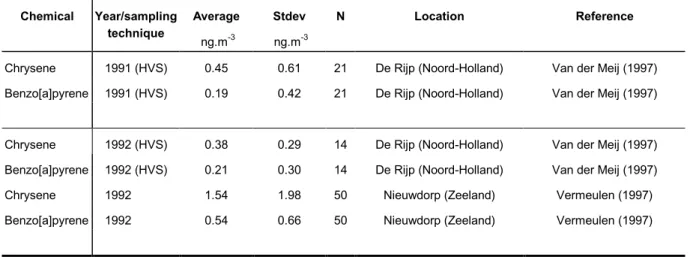
Several different authorities in The Netherlands monitor PAH concentrations in air. Measurements by the provincial authority of Noord-Holland were taken near industrial sources and Schiphol airport, as well as at a background station in the middle of the province Noord-Holland (De Rijp). Measurements of the advisory environmental service Rijnmond (DCMR-milieudienst) were taken at urban locations in Rotterdam. The provincial authority of Zeeland measured at a remote site, though influenced by industrial sources (Nieuwdorp). The National Institute of Public Health and the Environment in The Netherlands took air samples mainly at urban sites, which are influenced by traffic. For this study only concentrations measured at De Rijp and Nieuwdorp were used (Table 3.4). The concentrations of the selected PAHs at Nieuwdorp with an industrial burden, is approximately 3 to 5 times higher. Sampling by the province of Noord-Holland was carried out with a high volume sampler (HVS) with a PM10 inlet.

Table 3.4: Measured concentrations of PAHs in aerosols (Total Suspended particles) in 1991 and 1992 at regional sites in The Netherlands.

Chemical Year/sampling technique Average ng.m-3 Stdev ng.m-3 N Location Reference

Chrysene 1991 (HVS) 0.45 0.61 21 De Rijp (Noord-Holland) Van der Meij (1997) Benzo[a]pyrene 1991 (HVS) 0.19 0.42 21 De Rijp (Noord-Holland) Van der Meij (1997)

Chrysene 1992 (HVS) 0.38 0.29 14 De Rijp (Noord-Holland) Van der Meij (1997) Benzo[a]pyrene 1992 (HVS) 0.21 0.30 14 De Rijp (Noord-Holland) Van der Meij (1997) Chrysene 1992 1.54 1.98 50 Nieuwdorp (Zeeland) Vermeulen (1997) Benzo[a]pyrene 1992 0.54 0.66 50 Nieuwdorp (Zeeland) Vermeulen (1997)

HVS stands for the High Volume Sampling technique, which measures Total Suspended Particles (TSP). N is the number of measurements.

The National Precipitation Chemistry Monitoring Network consisted of 14 stations in 1991. At all stations samples were analysed for main components and heavy metals. Additionally, at three stations samples were taken to be analysed for organic microcomponents like alpha-hexachlorocyclohexane, gamma-alpha-hexachlorocyclohexane, hexachlorobenzene and thirteen representatives from the group of polycyclic aromatic hydrocarbons.

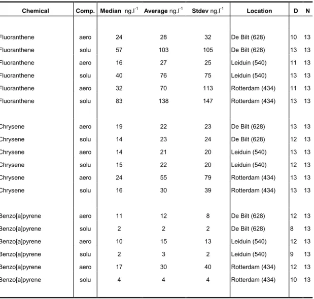
The results of these three sampling stations are presented in Table 3.5 for the selected chemicals. Sample values below the limit of detection (LOD) were substituted with half the LOD. Rain samples were taken with wet-only collectors during a four-week period and concentrations in the free soluble phase as well as bound to aerosols were determined.

Table 3.5: Measured concentrations of PAHs in rain in 1991 in The Netherlands.

Chemical Comp. Median ng.l-1 _{Average ng.l}-1 _{Stdev ng.l}-1 _{Location D N}

Fluoranthene aero 24 28 32 De Bilt (628) 10 13

Fluoranthene solu 57 103 105 De Bilt (628) 13 13

Fluoranthene aero 16 27 25 Leiduin (540) 11 13

Fluoranthene solu 40 76 75 Leiduin (540) 13 13

Fluoranthene aero 32 70 113 Rotterdam (434) 11 13

Fluoranthene solu 83 138 147 Rotterdam (434) 13 13

Chrysene aero 19 22 23 De Bilt (628) 13 13

Chrysene solu 14 23 24 De Bilt (628) 12 13

Chrysene aero 14 21 20 Leiduin (540) 13 13

Chrysene solu 15 22 20 Leiduin (540) 12 13

Chrysene aero 24 55 79 Rotterdam (434) 13 13

Chrysene solu 16 30 39 Rotterdam (434) 13 13

Benzo[a]pyrene aero 11 12 8 De Bilt (628) 12 13

Benzo[a]pyrene solu 2 2 2 De Bilt (628) 8 13

Benzo[a]pyrene aero 10 15 13 Leiduin (540) 12 13

Benzo[a]pyrene solu 2 3 2 Leiduin (540) 9 13

Benzo[a]pyrene aero 17 30 40 Rotterdam (434) 12 13

Benzo[a]pyrene solu 4 4 4 Rotterdam (434) 10 13

*Aben and Laan (1995).

Detection limits are 1 ng.l-1 _{for B[a]p and 0.3 ng.l}-1 _{for chrysene in solution (solu) and for the fraction associated with}

aerosols (aero): 0.3 ng.l-1 _{for fluoranthene. N is the number of measurements and D is the number of measurements above}

the detection limit.

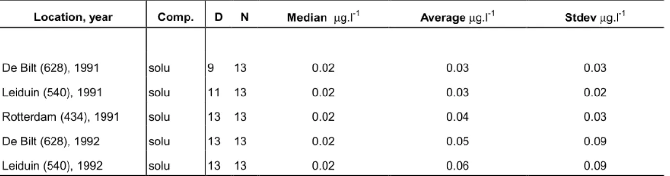
For lindane rain samples were taken with open precipitation collectors. This means that both wet and dry deposition was measured. Four-weekly samples were taken. Again for pragmatic reasons values below the LOD were replaced with LOD/2 (Table 3.6).

Table 3.6: Concentrations of lindane in precipitation in The Netherlands in 1991 and 1992*.

Location, year Comp. D N Median _µg.l-1 _Average

µg.l-1 _Stdev µg.l-1 De Bilt (628), 1991 solu 9 13 0.02 0.03 0.03 Leiduin (540), 1991 solu 11 13 0.02 0.03 0.02 Rotterdam (434), 1991 solu 13 13 0.02 0.04 0.03 De Bilt (628), 1992 solu 13 13 0.02 0.05 0.09 Leiduin (540), 1992 solu 13 13 0.02 0.06 0.09

* Buijsman and Stolk (1997A)

N is the number of measurements and D is the number of measurements above the detection limit.

The presence of pesticides in rainwater is studied in several research projects by provincial authorities and polder boards of which some of the results for lindane are presented in Table 3.7. We used the data for 1991 presented in Table 3.6.

Table 3.7: Measured concentrations of lindane in precipitation in The Netherlands*.

Location, year D N DL _µg.l-1 _Average

µg.l-1 _Max µg.l-1 Breda, 1988 2 3 0.001 0.0016 0.020 Fleverwaard, 1990,1991 5 80 0.01 0.018 0.030 Rijnland, 1988 36 36 0.01 0.14 0.68 Westland, 1988, 1989 21 21 0.001 0.027 0.11 Westland, 1990 3 3 - 0.016 0.021 Zuid-Holland, 1991, 1992 65 65 0.001 0.041 0.24 *Teunissen-Ordelman et al. (1996)

DL is the detection limit, N is the number of measurements and D is the number of measurements above the detection limit.

3.5 Water data

Concentrations in water and sediment as well as suspended matter are obtained from the Institute for Inland Water Management and Waste-Water Treatment (RIZA) and the National Institute for Coastal and Marine Management (RIKZ) which under the commission of the Department of Public Works executes a monitoring program called Monitoring the Condition of State waters (MWTL).

Monitoring data concerning chemicals in fresh water and seawater (see also Van Meerendonk et al., 1994, Phernambucq et al., 1996) are stored in the DONAR-database. Data were also available from the AQUAview database (Dagelet and Puijenbroek, 1997) which contains water quality data from the RIWA (RIWA, 1994).

The IJsselmeer (Andijk) and Markermeer Haringvliet and other major watersystems like Westerschelde and the rivers Rhine and Meuse are selected as ‘representative sites’ for the concentration in fresh water in The Netherlands. In the fresh water samples 25% (chrysene) and 52% (lindane and benzo[a]pyrene) of the samples was below the detection limit, see Table 3.8. Several statistical procedures can be used to calculate average concentration and the standard deviation. In these cases Quantile-Quantile plots were used to derive the location parameter and the spread of the distribution (D’Agostino and Stephens, 1986), see Appendix IV.

Table 3.8: Average concentrations of PAHs, lindane and tetrachloroethylene in major surface waters in The Netherlands, 1992*.

Chemical D N DL µg.l-1 _Average µg.l-1 _Stdev µg.l-1 Fluoranthene 224 271 0.006-0.02 0.037 0.036 Chrysene 53 70 0.01 0.019 0.014 Benzo[a]pyrene 112 213 0.004-0.01 0.017 0.064 Lindane 91 175 0.001-0.01 0.011 0.014 Tetrachloroethylene - 135 0.01 0.273 0.117

*Dagelet and Puijenbroek (1997); RIWA yearly report (1993 and 1994) and RIZA yearbook (1996).

DL is the detection limit, N is the number of measurements and D is the number of measurements above the detection limit.

Provinces and regional polder boards

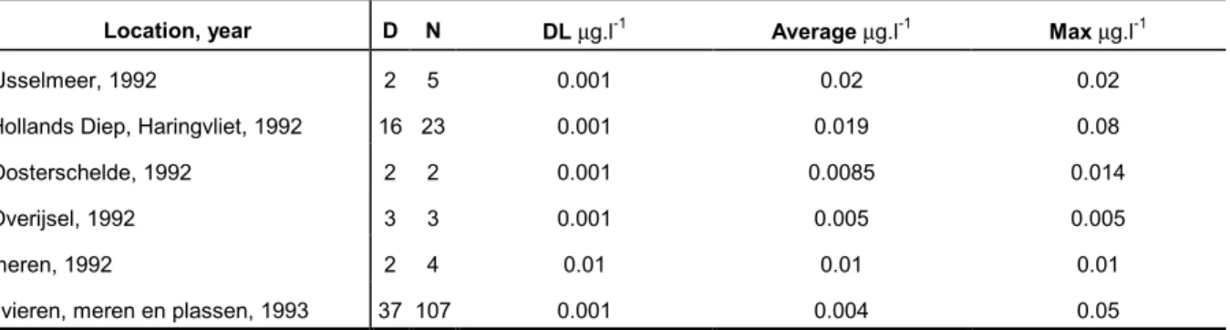
The coordination commission on the enforcement of the act on contamination of fresh surface waters in The Netherlands (CIW/CUWVO) makes an annual inventory (1992-1993) of the measurements performed by the water quality administrators. The data contain monitoring data of regional surface waters and the adjoining sediments. These data are under control of the RIZA-institute. For lindane a summary of these data is presented in Table 3.9 and 3.10. We used the results of Table 3.8, which are well in line with de data shown in Table 3.9 and 3.10

Table 3.9: Measured concentrations of lindane in major surface waters in The Netherlands*.

Location, year D N DL µg.l-1 _Average

µg.l-1 _Max

µg.l-1

IJsselmeer, 1992 2 5 0.001 0.02 0.02

Hollands Diep, Haringvliet, 1992 16 23 0.001 0.019 0.08

Oosterschelde, 1992 2 2 0.001 0.0085 0.014

Overijsel, 1992 3 3 0.001 0.005 0.005

meren, 1992 2 4 0.01 0.01 0.01

rivieren, meren en plassen, 1993 37 107 0.001 0.004 0.05

*Teunissen-Ordelman et al. (1996).

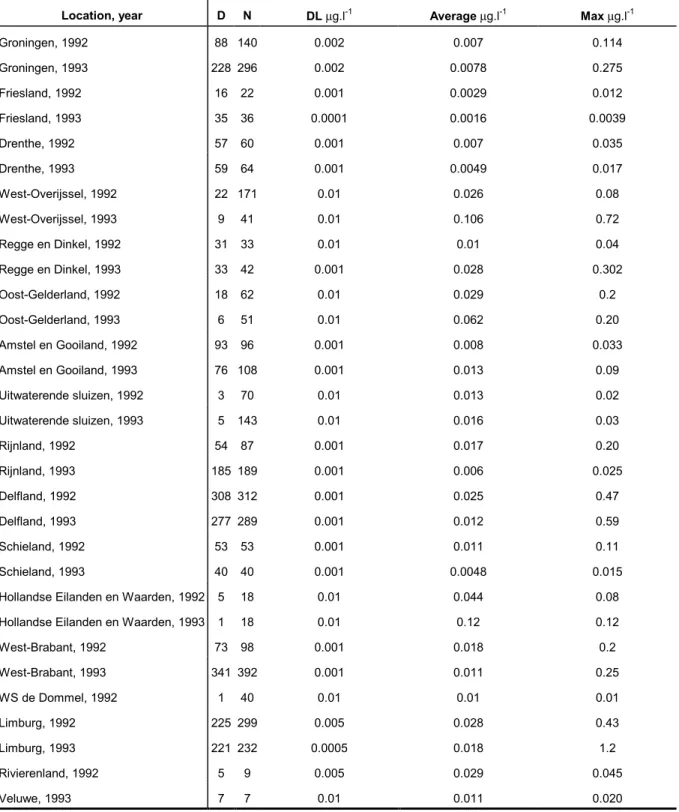
Table 3.10: Measured concentrations of lindane in regional surface water in The Netherlands*.

Location, year D N DL _µg.l-1 _Average

µg.l-1 _Max µg.l-1 Groningen, 1992 88 140 0.002 0.007 0.114 Groningen, 1993 228 296 0.002 0.0078 0.275 Friesland, 1992 16 22 0.001 0.0029 0.012 Friesland, 1993 35 36 0.0001 0.0016 0.0039 Drenthe, 1992 57 60 0.001 0.007 0.035 Drenthe, 1993 59 64 0.001 0.0049 0.017 West-Overijssel, 1992 22 171 0.01 0.026 0.08 West-Overijssel, 1993 9 41 0.01 0.106 0.72 Regge en Dinkel, 1992 31 33 0.01 0.01 0.04 Regge en Dinkel, 1993 33 42 0.001 0.028 0.302 Oost-Gelderland, 1992 18 62 0.01 0.029 0.2 Oost-Gelderland, 1993 6 51 0.01 0.062 0.20 Amstel en Gooiland, 1992 93 96 0.001 0.008 0.033 Amstel en Gooiland, 1993 76 108 0.001 0.013 0.09 Uitwaterende sluizen, 1992 3 70 0.01 0.013 0.02 Uitwaterende sluizen, 1993 5 143 0.01 0.016 0.03 Rijnland, 1992 54 87 0.001 0.017 0.20 Rijnland, 1993 185 189 0.001 0.006 0.025 Delfland, 1992 308 312 0.001 0.025 0.47 Delfland, 1993 277 289 0.001 0.012 0.59 Schieland, 1992 53 53 0.001 0.011 0.11 Schieland, 1993 40 40 0.001 0.0048 0.015

Hollandse Eilanden en Waarden, 1992 5 18 0.01 0.044 0.08

Hollandse Eilanden en Waarden, 1993 1 18 0.01 0.12 0.12

West-Brabant, 1992 73 98 0.001 0.018 0.2 West-Brabant, 1993 341 392 0.001 0.011 0.25 WS de Dommel, 1992 1 40 0.01 0.01 0.01 Limburg, 1992 225 299 0.005 0.028 0.43 Limburg, 1993 221 232 0.0005 0.018 1.2 Rivierenland, 1992 5 9 0.005 0.029 0.045 Veluwe, 1993 7 7 0.01 0.011 0.020 *Teunissen-Ordelman et al. (1996).

Suspended matter and sediment

Sediment monitoring data are available from five different sites, which are sampled once a year. Sediment concentrations are expressed on a dry weight basis (Table 3.11).

Table 3.11: Measured concentrations of PAHs in sediments [_µg.kg-1(dry)] of major and

regional surface waters in The Netherlands*.

Chemical Average mg.kg-1 _{(dry). Stdev N D}

Fluoranthene 1.08 1.23 6 5

Chrysene 0.49 0.52 6 5

Benzo[a]pyrene 0.59 0.63 6 5

Lindane <0.001 - 44 0

*RIZA, Yearbook (1995).

N is the number of measurements and D is the number of measurements above the detection limit.

Concentrations in suspended matter are monitored on a more regular basis through out a year. Average concentrations for the major surface waters in The Netherlands are presented in Table 3.12

Table 3.12: Measured concentrations of PAHs in suspended solids [µg.kg-1_{(dry)] in major}

surface waters in The Netherlands in 1992*.

Chemical Average mg.kg-1 (dry) Stdev N D

Fluoranthene 1.33 1.33 93 87

Chrysene 0.68 0.56 92 91

Benzo[a]pyrene 0.73 0.68 93 91

Lindane 0.002 0.003 97 81

*RIZA, DONAR-data base.

N is the number of measurements and D is the number of measurements above the detection limit.

3.6 Soil quality data

Concentrations in the soil are measured in the Dutch National Soil Quality Monitoring Network (LMB). The network is one of the responsibilities of the Laboratory of Soil and Groundwater Research at the National Institute of Public Health and the Environment. Soil and Groundwater quality assessment in The Netherlands for different combinations of soil use (grassland, arable land, forest soils) and soil types (sand, fluvial and marine clay, peat and loam) is one of their main objectives. Concentration data on PAHs, PCBs (Appendix III), pesticides and heavy metals for agriculturally used soils and natural soils in 1992, 1993 and 1994 are available (Lagas and Groot, 1996; Groot and van Swinderen, 1993 and Groot et al., 1996). Average concentrations and standard deviations of selected chemicals for different agricultural soil uses are summarised in Table 3.13.

Table 3.13: Measured concentrations of PAHs and lindane [µg.kg-1_{(dry)] in top level (10 cm)}

of agricultural soils in The Netherlands in 1992 *.

Chemical Grassland Arable land Maize culture Bulb growing Fruit culture avg std avg std avg std avg std avg std Lindane 0.64 0.36 0.80 0.66 1.28 0.86 0.17 - 0.30

-Chrysene 64 71 20 9 25 20 13 - 96 -Pyrene 96 124 29 14 35 30 17 - 142 -Benzo[a]pyrene 56 68 16 8 19 15 8 - 60

-*Lagas and Groot (1996).

3.7 Summary

The data from the various monitoring networks in The Netherlands provided concentration data for five substances to construct concentration ratios for adjoining compartments which, are assumed to be representative for The Netherlands. Air(aerosol)-water concentration ratios can be deduced from data on benzo[a]pyrene, pyrene and tetrachloroethylene (tetra). Rain-water concentration ratios can be derived from data on benzo[a]pyrene, fluoranthene, pyrene and lindane. Data about lindane and benzo[a]pyrene, fluoranthene and pyrene also could be used to derive water-sediment and water-suspended matter concentration ratios. Air(aerosol)-soil concentration ratios can be estimated for benzo[a]pyrene and pyrene and rain-Air(aerosol)-soil

concentration ratios can be derived for benzo[a]pyrene, fluoranthene, pyrene and lindane. The data are summarised in Table 3.14.

Table 3.14: Measured concentrations of selected compounds used in validation procedure.

measured concentrations substance compartment units average median stdev

Tetrachloroethylene water _µg.l-1 _{0.273 0.185 0.413}

air _µg.m-3 _{0.331 0.220 0.399}

Lindane rainwater _µg.l-1 _{0.055 0.020 0.094}

freshwater _µg.l-1 _{0.011 0.005 0.014}

sediment _µg.kg-1_{(dry) < 1.00 -}

-suspended matter _µg.kg-1_{(dry) 2.19 1.00 2.85}

agricultural soil _µg.kg-1_{(dry) 0.67 0.55 0.45}

Benzo[a]pyrene aerosols ng.m-3 0.38 0.21 0.55

rainwater ng.l-1 22.8 13.8 27.0

freshwater _µg.l-1 _{0.017 0.008 0.064}

sediment mg.kg-1(dry) 0.59 0.45 0.63

suspended matter mg.kg-1(dry) 0.73 0.60 0.68 agricultural soil _µg.kg-1_{(dry) 40.8 22.0 57.1}

Chrysene aerosols ng.m-3 0.96 0.48 1.49

rainwater ng.l-1 58.8 31.0 70.5

freshwater _µg.l-1 _{0.018 0.010 0.014}

sediment mg.kg-1(dry) 0.49 0.35 0.53

suspended matter mg.kg-1(dry) 0.68 0.50 0.56 agricultural soil _µg.kg-1_{(dry) 51.9 31.9 60.5}

Fluoranthene aerosols ng.m-3

rainwater ng.l-1 147 95 172

freshwater _µg.l-1 _{0.037 0.026 0.036}

sediment mg.kg-1(dry) 1.07 0.70 1.22

suspended matter mg.kg-1(dry) 1.33 1.10 1.32 agricultural soil _µg.kg-1_{(dry) 112 60 152}

4. M

SimpleBox version 2.0 was used for the calculation of the probability distributions of steady-state concentration ratios. The SimpleBox settings must be adjusted to simulate the

environment in which the measurements are carried out. The various sources and types of uncertainty and the specific settings of both SimpleBox and the Monte Carlo simulation -which will be performed to examine the range of the SSCRs- are presented in this chapter.

4.2 Monte Carlo Simulations

Monte Carlo simulation is a useful tool to get insight in the uncertainties of the steady state concentration calculations of SimpleBox. The Monte Carlo simulation is performed with Crystal Ball, an add-in for Microsoft Excel (Decisioneering, 1993). This method samples values of the input parameters at random from the probability distribution for each input parameter (sampling method: Latin hypercube).

4.3 Variability and uncertainty

In this research we considered both uncertainty due to empirical inaccuracy, lack of data and uncertainty due to temporal variability. Spatial variability cannot be applied simply because spatial variability is not modelled within SimpleBox. The boxes within SimpleBox are considered to be homogeneous, so one value of a parameter is valid for the entire box. Uncertainty due to temporal variability is operational. Since an average over a box may vary in time.

Model domain parameters may vary temporally. For example, mixing height of air and mean water depth are model domain parameters but have no domain scenario uncertainty since they are well defined, but still uncertain due to unavoidable empirical uncertainty and lack of data. Uncertainty due to lack of data may be explained by estimating a value and an uncertainty factor or a range in case there are not enough data.

We assumed that the variability in the model estimates is the result of the uncertainty in selected input parameters, due to:

• empirical inaccuracy with respect to substance properties • inaccurate information on emissions

• lack of data and temporal variability with respect to model domain parameters as mixing height of air and water depth. Meteorological data and other data that describe the environment (e.g. windspeed and rainfall) are represented as variable parameters. • lack of knowledge about interactions between the substance and its environment

These uncertainties are thought to propagate, causing uncertainty in the model output. Information on the distribution types for the different environmental settings etc. is extracted from the sensitivity/uncertainty analysis of SimpleBox by Etienne et al. (1997), see Table 4.2. The distributions are defined by assigning a type of distribution, normal, lognormal triangular etc. and specific distribution parameters. Depending on the importance of its influence on the model output and the availability of data it is required to define the right distribution. The final result is a probability distribution (= output uncertainty) of the SSCR which will be compared with the distribution of concentration ratios, which were derived from measured concentrations at various locations over The Netherlands over one or two years.

4.4 Model settings for The Netherlands

The SimpleBox 2.0 defaults of the regional scale simulate a typical Western-European region. The model parameters are adjusted to model The Netherlands. In this case, we have decided that the dimensions of the system (The Netherlands) are not subject to Monte Carlo sampling. Thus, the system area and area fractions are part of the scenario. Table 4.1 gives the scenario assumptions for this validation study. We made three exceptions: mixing height of air, the depth of the fresh surface water compartment and the depth of the soil compartments. The mixing height of air and the depth of the fresh surface water compartment have a large

influence on the model output as was shown by Etienne et al. (1997). The mixing height of air and the depth of the water compartment determine the volume of the air and fresh surface water compartment, respectively. The mixing height varies temporally, it shows daily and seasonal variation. For water depth typical representative values were used based on what can be found for real water systems. The depth of the soil compartment is calculated from the chemical specific penetration depth (Brandes et al., 1996; Cowan et al. 1995). The vegetation compartment was turned off during the model calculations.

The time scale for temporally varying parameters as WINDspeed, mixing layer height, and

TEMPERATURE is set to 24 hours-daily average values were taken. For the RAINRATE

monthly average values typical for The Netherlands were applied. This is believed to be more appropriate concerning the sampling duration. Other distributions are chosen based on expert judgement of the authors.

Table 4.1: Scenario assumptions.

Parameter name Unit Regional

SYSTEMAREA km2 84,000*

Area fresh water km2 _{4,200 (5%)}

Area sea water km2 _{42,000 (50%)}

Area natural soil km2 16,800 (20%)

Area agricultural soil km2 _{20,200 (24%)}

Area urban soil km2 _{840 (1%)}

Depth sea water m 25

Average residence time sea water d 76

*The area soil + area fresh water in The Netherlands is 50% of the total SYSTEMAREA, the other fraction is sea water.

- Chemical dependent penetration depth in soils

Introducing the chemical dependent penetration depth gives a more accurate estimate of the exchange between the soil compartment and the air compartment. Within SimpleBox 2.0 (Brandes et al., 1996) the diffusion coefficients have default values of 11·10-6 and

11·10-10 [m2.s-1] for soil air and water, respectively. They are used for the calculating the chemical dependent penetration depth for soils. It is thought to be more accurate to make the diffusion coefficients in air and water substance dependent, although no sensitivity analysis was performed.

- Tropospheric OH-radical concentration

For most substances reaction with hydroxyl radicals is the major atmospheric removal pathway although transformation pathways like reaction with ozone and the night-time

reaction with nitrate-radicals also contribute. Hydroxyl radical reaction rate constants are used in estimating the atmospheric degradation. These reaction rate constants are calculated by the contribution method by Atkinson (Atkinson, 1988) and were reported by Howard (1991b). The atmospheric degradation based on hydroxyl radical reaction rate is not only dependent on atmospheric hydroxyl radical concentrations, which vary seasonally as will be shown below, but is also temperature dependent. Because of lack of data on the substances we studied, we use as an approximation the rule of thumb known as Van ‘t Hoff’s law.

It states that in general the reaction rate lowers by half, respectively doubles with every 10 degrees of temperature drop or rise. Reaction rates estimated by Atkinson’s method refer to room temperature (25 °C).

Atmospheric hydroxyl radical concentrations change daily and seasonally. Hydroxyl radicals are generated by atmospheric photochemical reactions, hence the daily and seasonal changes result from the intensity of the solar radiation which reaches the earth (troposphere).

Consequently atmospheric hydroxyl concentrations drop to zero at night. Hydroxyl radical concentrations differ by latitude, concentrations in the tropic regions are generally higher than atmospheric concentrations at the Northern or Southern part of the hemisphere. Many studies were aimed at measuring tropospheric hydroxyl radical concentrations. An overview is given by Hewitt and Harrison (1985) and GDC (1992). In addition to these measurements several models (Lu and Khalil, 1991; Perner et al., 1987 and Crutzen and Gidel, 1983) have been developed to predict tropospheric hydroxyl radical concentrations. From these measuring

results and model predictions, monthly 24-hour average tropospheric hydroxyl radical concentrations at the Northern hemisphere are derived. A custom distribution function with continuous ranges is used to model the monthly variation of the tropospheric hydroxyl radical concentration. Characteristics of the custom distribution of hydroxyl radicals are reported in Appendix V.

- Correlations

The parameter TEMPERATURE on the regional and continental spatial scale is assumed to correlated with a correlation coefficient of 0.9. Similarly, the degradation half-lives in the compartments of the spatial scales are correlated with a correlation coefficient of 0.9.

WINDspeed and HEIGHTair are also correlated with a correlation coefficient of 0.85 (Etienne

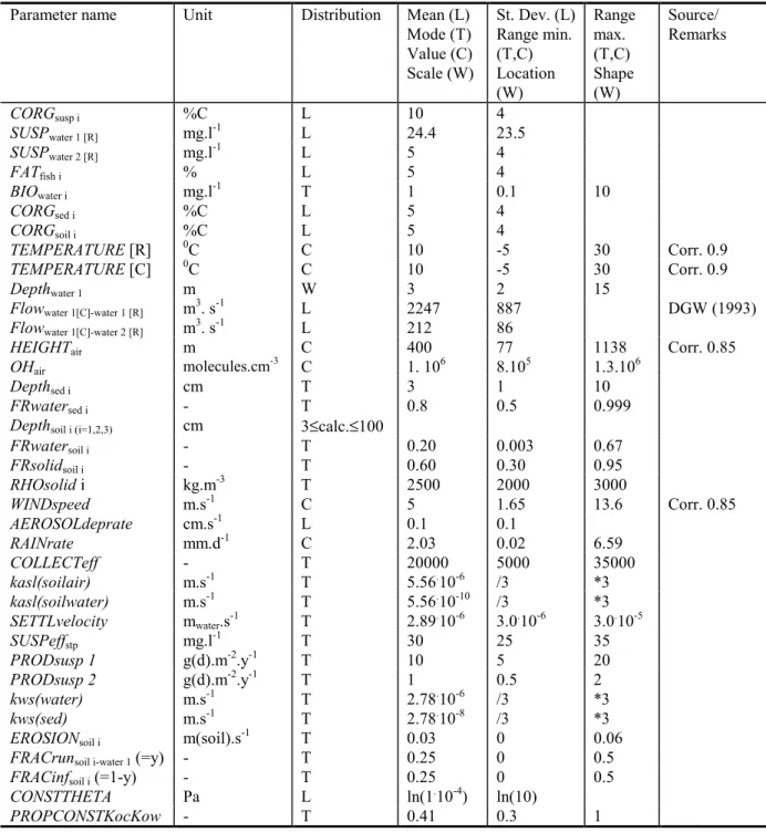
Table 4.2: Characteristics of the probability distributions of non-compound-specific input parameters.

Parameter name Unit Distribution Mean (L) Mode (T) Value (C) Scale (W) St. Dev. (L) Range min. (T,C) Location (W) Range max. (T,C) Shape (W) Source/ Remarks CORGsusp i %C L 10 4 SUSPwater 1 [R] mg.l-1 L 24.4 23.5 SUSPwater 2 [R] mg.l-1 L 5 4 FATfish i % L 5 4 BIOwater i mg.l-1 T 1 0.1 10 CORGsed i %C L 5 4 CORGsoil i %C L 5 4 TEMPERATURE [R] 0C C 10 -5 30 Corr. 0.9 TEMPERATURE [C] 0_{C C 10 -5 30 Corr. 0.9} Depthwater 1 m W 3 2 15

Flowwater 1[C]-water 1 [R] m3. s-1 L 2247 887 DGW (1993)

Flowwater 1[C]-water 2 [R] m3. s-1 L 212 86

HEIGHTair m C 400 77 1138 Corr. 0.85

OHair molecules.cm-3 C 1. 106 8.105 1.3.106

Depthsed i cm T 3 1 10

FRwatersed i - T 0.8 0.5 0.999

Depthsoil i (i=1,2,3) cm 3≤calc.≤100

FRwatersoil i - T 0.20 0.003 0.67 FRsolidsoil i - T 0.60 0.30 0.95 RHOsolid i kg.m-3 _{T 2500 2000 3000} WINDspeed m.s-1 _{C 5 1.65 13.6 Corr. 0.85} AEROSOLdeprate cm.s-1 _{L 0.1 0.1} RAINrate mm.d-1 _{C 2.03 0.02 6.59} COLLECTeff - T 20000 5000 35000 kasl(soilair) m.s-1 _{T 5.56}.₁₀-6 _{/3 *3} kasl(soilwater) m.s-1 _{T 5.56}.₁₀-10 _{/3 *3} SETTLvelocity mwater.s-1 T 2.89.10-6 3.0.10-6 3.0.10-5 SUSPeffstp mg.l-1 T 30 25 35 PRODsusp 1 g(d).m-2_.y-1 _{T 10 5 20} PRODsusp 2 g(d).m-2_.y-1 _{T 1 0.5 2} kws(water) m.s-1 _{T 2.78}.₁₀-6 _{/3 *3} kws(sed) m.s-1 _{T 2.78}.₁₀-8 _{/3 *3}

EROSIONsoil i m(soil).s-1 T 0.03 0 0.06

FRACrunsoil i-water 1 (=y) - T 0.25 0 0.5

FRACinfsoil i (=1-y) - T 0.25 0 0.5

CONSTTHETA Pa L ln(1.₁₀-4_{) ln(10)}

PROPCONSTKocKow - T 0.41 0.3 1

The distributions are indicated as Normal, Lognormal, Triangular, Weibull and Custom. The various distributions are characterised by different parameters: Normal and Lognormal by the mean and a standard deviation, triangular by mode and range etcetera.

4.5 Chemical compound properties

Chemical properties of the selected chemicals (physical-chemical properties and degradation rates) are obtained from different literature sources. Most common sources of chemical properties are: