October 2004 ECN-C--04-085
Realised energy savings 1995 -2002
According to the Protocol Monitoring Energy Savings
P.G.M. Boonekamp, ECN A. Gijsen, RIVM/MNP H.H.J. Vreuls, SenterNovem
Milieu- en Natuurplanbureau
Acknowledgement
This study was carried out for the Dutch Ministry of Economic Affairs by ECN-Policy Studies, in collaboration with the Netherlands Environmental Assessment Agency (MNP) of RIVM and SenterNovem. The work has been accomplished at ECN under project number 7.7543, the re-port number is ECN-C--04-085, the RIVM/MNP rere-port number is 773001028.
This report is the translation of a Dutch report that was published in September 2004 (ECN re-port number ECN-C--04-016 and RIVM/MNP-rere-port number 773001027). The translator, Mrs M.E. Kamp of ECN, is gratefully acknowledged for her efforts.
Abstract
In this report the realized energy savings in the Netherlands for the period 1995-2002 are pre-sented for the sectors households, industry, agriculture, services, transportation, refineries and electricity and for the national level. First a short description is given of the ‘Protocol Monitor-ing Energy SavMonitor-ings’, a common methodology and database for calculatMonitor-ing the amount of energy savings that was set up earlier by four Dutch institutes CPB, ECN, Novem and RIVM. Results are presented for savings on final energy use, conversion in end-use sectors (co-generation) and for conversion in the energy sector. National savings of 1.0% per year are found, with a decreas-ing tendency in recent years.
Much attention is given to the uncertainty margins that result from the uncertainty in the input data and the ‘quality’ of the variable that is used to calculate the reference energy use (without savings). It turns out that it is impossible to supply a reliable savings figure for final energy use in the services sector. On the other hand, the savings from better conversion can be calculated quite well. Overall, a margin of +/-0.3% is found for the national yearly savings figure.
Next to savings, an analysis has also been made of volume and structural effects with respect to energy consumption, energy intensity developments and other relevant factors in different sec-tors. Finally, savings have been put in perspective: a comparison is made with the savings of the EU-countries, the contribution of savings to the reduction of the CO2 emissions is examined and
CONTENT
LIST OF FIGURES 4
LIST OF TABLES 5
SUMMARY 7
1. INTRODUCTION 11
2. PROTOCOL METHOD IN BRIEF 12
2.1 Definition of energy savings 12
2.2 Volume, structure and saving effects 13
2.3 Energy consumption quantities 15
2.4 Calculation of savings per sector and national 19
3. ENERGY SAVINGS 1995 - 2002 21
3.1 Calculation method and input data 21
3.2 Savings per sector and national 21
3.3 Volume, structure and saving effects 22
3.4 Uncertainty margins in the results 22
3.5 Trend in development of savings 23
4. SECTORAL ENERGY CONSUMPTION AND SAVINGS TRENDS 24
4.1 Introduction 24
4.2 Households 25
4.3 Industry (including construction) 28
4.4 Agriculture and horticulture 33
4.5 Services sector 36
4.6 Transportation 39
4.7 Refineries 42
4.8 Electricity supply 44
4.9 Other energy companies 48
4.10 Total energy consumption 48
5. ENERGY SAVINGS IN PERSPECTIVE 53
5.1 International comparison 53
5.2 Energy savings and CO2 emission reduction 54
5.3 Savings through cogeneration 54
5.4 Other evaluations 56
LITERATURE 57
ANNEX A SECTORAL DIVISION PROTOCOL ENERGY SAVINGS 59
ANNEX B COMPARISON WITH PREVIOUS EVALUATIONS 60
ANNEX C UNCERTAINTY ANALYSIS SAVINGS DATA 62
LIST OF FIGURES
Figure S.1 Energy consumption per capita and per € GDP for 1990-2002 8
Figure 2.1 Energy consumption, reference consumption and savings 12
Figure 2.2 Energy consumption developments and volume, structure and saving effect 14
Figure 2.3 Relation energy use with final energy consumption and primary energy
consumption 17
Figure 2.4 Energy use and energy consumption in primary units for cogeneration and
separate generation of heat and electricity 18
Figure 3.1 Decomposition of change in national energy consumption 1995-2002 22
Figure 4.1 Volume, structure and saving effects for Households 1995-2002 26
Figure 4.2 Heat and electricity intensity for Households 1990-2002 27
Figure 4.3 Primary energy consumption per energy function for Households (1990=100) 27
Figure 4.4 Volume, structure and saving effects in Industry (including construction) 1995-2002 29
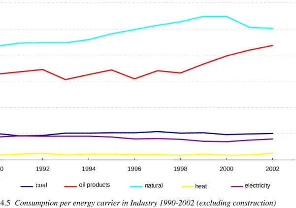
Figure 4.5 Consumption per energy carrier in Industry 1990-2002 (excluding construction) 30
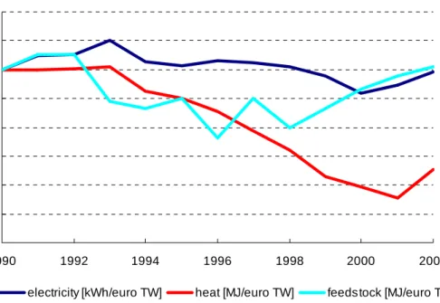
Figure 4.6 Electricity, heat and feedstock intensity for Industry 1990-2002 31
Figure 4.7 Final intensity of electricity consumption in industrial sectors [MJ/€] 32
Figure 4.8 Final intensity of heat consumption in industrial sectors [MJ/€] 33
Figure 4.9 Volume, structure and saving effects in Agriculture and horticulture 1995-2002 34
Figure 4.10 Electricity and heat intensity in Agriculture and horticulture 1990-2002 35
Figure 4.11 Volume, structure and saving effects in the Services sector 1995-2002 37
Figure 4.12 Electricity and heat intensities for Services 1990-2002 38
Figure 4.13 Volume, structure and saving effects in Transportation 1995-2002 40
Figure 4.14 Fuel and electricity intensities of passenger and freight transport 1990-2002 (index, 1990=100) 41
Figure 4.15 Volume, structure and saving effects in Refineries 1995-2002 43
Figure 4.16 Electricity and fuel intensities for Refineries 1990-2002 44
Figure 4.17 Composition of electricity supply 1990-2002 45
Figure 4.18 Conversion efficiency developments per type of power plant 1990-2002 46
Figure 4.19 Total efficiency of electricity supply, including or excluding heat delivery, waste incineration or import 47
Figure 4.20 Statistical and temperature corrected energy consumption in the Netherlands for 1990-2002 49
Figure 4.21 Energy consumption per capita and per unit of GDP 50
Figure 4.22 Development of energy consumption per sector 1990-2002 51
LIST OF TABLES
Table S.1 Energy savings 1995-2002 according to protocol method 7
Table S.2 Trend in national savings as of 1995 7
Table S.3 Development of GDP, energy consumption and energy intensity 8
Table 3.1 Saving results for the period 1995-2002 21
Table 3.2 Trend in national savings as of 1995 23
Table 4.1 Used multiplication factors per energy carrier 24
Table 4.2 Development of savings for Households, according to the protocol method 25
Table 4.3 Growth of expenditures and electricity consumption for Households 28
Table 4.4 Development of savings in Industryaccording to the protocol method 29
Table 4.5 Annual growth rate value added of industry and energy-intensive subsectors 32
Table 4.6 Development of savings in Agriculture and horticulture, according to the
protocol method 34
Table 4.7 Development of savings in the Services sector, according to the protocol method 36
Table 4.8 Relation between growth of value added and final energy consumption in
Services 38
Table 4.9 Energy consumption categories and ERG in Transportation 39
Table 4.10 Development of savings in Transportation, according to the protocol method 39
Table 4.11 Development of savings in Refineries, according to the protocol method 42
Table 4.12 Input, output and overall efficiency of power plants 1990-2002a 45 Table 4.13 Relation between input and output for waste incineration 46
Table 4.14 Input and output and efficiency of cogeneration production 46
Table 4.15 Input, output and efficiency of coke production 48
Table 4.16 Trends in growth of GDP, energy consumption and energy intensity 50
Table 4.17 Build-up of the national structure effect in the protocol method 52
Table 5.1 Comparison of energy consumption trends for the Netherlands and the EU 53
Table 5.2 Total increase in energy efficiency for 1995-2002 in the Netherlands and the EU 53
Table 5.3 Savings from cogeneration production 1990-2002 55
Table 5.4 Energy efficiency trends in Agriculture and Horticulture, according to PME
and LEI 56
Table A.1 Division of energy consumers according to CBS and current / original protocol 59
Table B.1 Comparison of savings data of the three Protocol evaluations 60
Table B.2 Volume, structure and saving effect period 1990-2000 61
Table B.3 Energy savings for 1990 - 1999/2000/2001 61
SUMMARY
At the request of the Dutch ministry of Economic Affairs, the institutions CPB, ECN, Novem1 and RIVM/MNP, with assistance of CBS, developed a common method for the calculation of the realised energy savings, the so-called ‘Protocol Energy Savings’. Energy savings for 1990 to 2000 and 2001 respectively were reported in previous publications. This report covers the results for the period 1995-2002.
Realised savings
When calculating savings according to the Protocol, a distinction is made between: • final energy consumption in end use sectors and refineries,
• conversion in end use sectors, among which cogeneration production, • conversion in the electricity supply (see Table S.1).
Table S.1 Energy savings 1995-2002 according to protocol method [%/year] National Industrya Services Households Agriculture
and horticulture
Transportb Refineries
Final energy 0.7 0.8 0.0 1.2 1.1 0.4 0.8
Conversion 0.2 0.2 0.5 0.0 0.6 0.0 0.2
Total end users 0.9 1.0 0.5 1.2 1.7 0.4 1.0
Supply 0.1
National 1.0
a
Including construction.
b
Including energy consumption mobile equipment.
The savings on final energy consumption in different sectors result in national savings of 0.7% annually. If savings from cogeneration are included, savings amount to 0.9%. The savings in electricity supply add 0.1%-point to the total national savings of 1.0% annually. It must be noted that it was impossible to establish a final savings figure for Services due to unreliable energy consumption data and unavailability of variables to determine the reference consumption. In this case the final savings were set at nil. The uncertainty in the national savings figure amounts to 0.3 %-point. With a certainty of 95% it can be said that national savings lie between 0.7% and 1.3%. The figures on final energy consumption for the separate sectors have a larger uncertainty range. The figures for conversion, however, are relatively firm.
Table S.2 illustrates the recent trends in national savings. From these data it can be concluded that the level of savings is decreasing gradually, both in final energy consumption and in cogeneration and power plants. This trend is visible in various sectors and is also supported by additional analyses (see Chapter 4).
Table S.2 Trend in national savings as of 1995
[%/year] 1995-2000 1995-2001 1995-2002
Final energy consumption 0.8 0.8 0.7
Cogeneration and power plants 0.4 0.3 0.3
Total 1.2 1.1 1.0
1
Energy consumption developments
The analysis covers the period starting from 1990, in coherence with previously defined policy. The energy consumption trend is not only influenced by savings but also by volume developments, such as economic growth, and structural developments such as sectoral shifts, more appliances per household, heavier cars and more air-conditioning in offices. The growth of the gross domestic product (GDP) would, everything else unaltered, have led to an annual increase of in energy consumption of 2.6%. This increase is lowered by structural developments with 0.4%-point. Taking into account the 1.0% savings, the total energy consumption increases with 1.2% per year (see Table S.3, last column).
The energy intensity, defined as the relation between economic growth and energy consumption, appears to decrease more rapidly in case of a larger economic growth (see Table S.3). As a result, energy consumption does not increase much faster in a period with a larger than average economic growth compared to periods with a smaller economic growth.
Table S.3 Development of GDP, energy consumption and energy intensity
[%] 1990-1994 1994-1998 1998-2002 1990-2002
GDP growth 1.9 3.6 2.2 2.6
TPES growth 1.0 1.3 1.3 1.2
Energy-intensity -0.9 -2.2 -0.9 -1.3 to -1.4
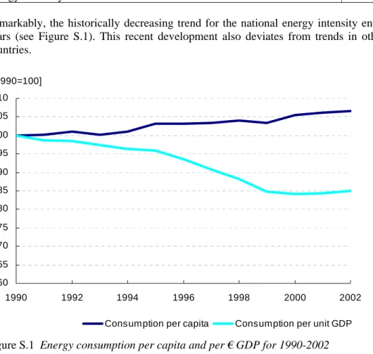
Remarkably, the historically decreasing trend for the national energy intensity ended in recent years (see Figure S.1). This recent development also deviates from trends in other European countries. 60 65 70 75 80 85 90 95 100 105 110 1990 1992 1994 1996 1998 2000 2002 [1990=100]
Consumption per capita Consumption per unit GDP
Figure S.1 Energy consumption per capita and per € GDP for 1990-2002
Savings in power plants and cogeneration production
The average conversion efficiency of power stations increased by 1995 due to the start of the newer and very efficient Eems Power Plant. After 1998, efficiency is decreasing again as a result of energetically less optimal deployment of production capacity. This probably relates to the abandonment of the national optimisation scheme for the deployment of power plants of Sep and the substantial growth in imports of electricity.
Total savings due to (non-central) cogeneration production increased rapidly as of 1990. After reaching a maximum value in 1998 the savings decreased again. Savings from cogeneration have been determined using the average power production efficiency in the base year. If the current average efficiency would be chosen, lower savings are found as of 1995 but relatively higher savings as of 1998 (due to the decreased average efficiency of power plants).
CO
2emission reduction of savings
The avoided CO2 emission, resulting from realised energy savings since 1990, amounted to
14-16 Mton or approximately 8% of the total Dutch emissions. About 3-4 Mton of this amount is the result of more efficient conversion (cogeneration and power plants); the rest stems from savings on final energy consumption. This emission reduction is partly due to energy policy and partly the result of autonomous technological advancement. Compared to the avoided emissions of renewable energy production, approximately 3 Mton, savings have contributed five times more to the emission reduction than renewable energy.
International comparison of realised savings
The saving figures have been compared with the realised efficiency improvements in the EU as determined in the Odyssee project. For households the Netherlands show higher savings than the EU in total. For industry and transportation it is difficult to draw firm conclusions because of the differences in method. Overall it may be concluded that the Netherlands do not score worse than EU countries as a whole.
Necessary improvement of the monitoring
For industry a new method has been used to calculate energy savings that is based on detailed physical production data. This appears to be a valuable alternative for the prior information derived from the LTA-monitoring that was ended recently. However, this does not constitute a solution for refineries where necessary data for a proper division of energy consumption development into saving- and structure effects are missing (changes in crude oil input, use of semi manufactured products and changes in output mix). As for the sector Services, reliable energy consumption data from distribution companies databases have to be awaited. Also a substantial effort is needed, for example by means of a survey, to determine the reference consumption and savings.
1. INTRODUCTION
Monitoring energy savings
Dutch figures on energy consumption and savings have not been calculated and presented in a uniform manner in the past, by policy makers (Ministries of Economic Affairs and Spatial Plan-ning, Housing and the Environment) as well as by the institutes involved (CPB, ECN, Novem2 and RIVM/MNP). In addition, little attention has been paid to the uncertainties in the data. By request of the Ministry of Economic Affairs the institutes have elaborated on a joint method laid down in the report ‘Protocol Monitoring Energy savings (PME)’ (Boonekamp, 2001). The pro-tocol defines the quantities and system boundaries to be used. The report also describes the ap-plied decomposition method and the calculation scheme, including the variables and data needed.
Performed evaluations
Since the establishment of the protocol, results on savings have been presented twice:
• for the period 1990-2000, as part of the report ‘Energy savings trends 1990-2000’ (Boone-kamp, 2002),
• for the period 1990-2001, at a workshop organised by the platform (Vreuls, 2003). In addition, a publication was devoted to uncertainty margins (Gijsen, 2003).
Changes in the protocol method
This report presents the realised savings for 1995-2002. As data from the Long Term Agree-ments (LTA) were no longer available for calculating industrial savings as of 2000, a new ap-proach had to be used (Neelis, 2004). An outcome of this new method was a shift in base year from 1990 to 1995. Moreover, the sector definitions were adjusted to the new division, agreed upon as part of the formulation of sectoral indicative targets for CO2 emissions. Furthermore,
the opportunity was seized to improve the protocol method in a number of other sectors and to provide for a better linking of the calculation scheme to the energy data from the MONIT sys-tem (Boonekamp, 2004). Finally, the presentation of results on savings has been extended with information on general energy consumption developments over a longer period of time and in a broader framework.
Reading instructions
Given the substantial changes an extended report is published. Chapter 2 summarises the previ-ously established protocol method. Chapter 3 presents the savings for the period 1995-2002, in-cluding a trend and uncertainty analysis. Chapter 4 elaborates on energy consumption develop-ments per sector and elucidates the protocol method into more detail. Moreover, developdevelop-ments are explained as good as possible. Finally Chapter 5 sheds a light on the savings from different perspectives, including a comparison with abroad and the emission reduction of savings.
2
2.
PROTOCOL METHOD IN BRIEF
2.1
Definition of energy savings
General definition
Energy is saved when the same activities are performed or the same functions are provided with less energy consumption. The energy savings are expressed in absolute units (PJ) or relative (%) to the energy consumption before the savings were achieved.
Determination of savings using the reference consumption
Energy savings cannot be measured or observed directly because it entails energy that has not been used. Energy savings must therefore be determined in a different way. The protocol makes use of the so-called reference consumption that is equal to the theoretical energy consumption in case no energy savings would take place. By definition energy savings are the difference be-tween realised energy consumption and reference consumption in the end year (see Figure 2.1). In this way the problem of calculating energy savings is replaced by the problem of determining the correct reference consumption.
Consumption Reference consumption
Base year Reference year
Saving
Mutation
Figure 2.1 Energy consumption, reference consumption and savings
Energy relevant quantities for the determination of the reference consumption
The reference consumption is determined by linking it to a so-called energy relevant variable (ERG in Dutch). The changes over time for such a variable determine the decrease or increase of the reference consumption. The ERG is connected to the activities, the performances or the social needs that require energy. It is expressed in physical, social or economic units, e.g. tons of steel production in the industrial sector or the number of households in the households sector. The definition and determination of savings thus entails choosing the relevant physical and socio-economic quantities. At a high aggregation level it is often not possible to use just one variable for calculating the reference consumption. Industry, for example, does not produce one single product where the production level would qualify as a good energy-relevant variable. In order to find suitable quantities lower des-aggregation levels of energy consumption have to be
sought, e.g. space heating in households or fertilizer production in the chemical industry. Some examples of ERGs for various reference consumptions are:
• aluminium production for the electricity consumption of the non-ferro sub-sector of base metal industry,
• the floor area of offices for the gas consumption of space heating in the services sector, • hot water consumption of households for the gas consumption of tap water systems in
households.
Base year and end year
Evaluation of energy savings entails a time span: the realised savings are always determined for a certain period of time. Therefore the protocol uses a base year and an end year (see Fi-gure 2.1). In the base year, reference consumption and actual energy consumption are the same by definition. The difference between the two in the end year constitutes the savings after the base year.
Change in energy consumption and savings
The change in energy consumption is equal to the difference between observed energy con-sumption in the base year and that in the end year (see Figure 2.1). Energy savings lead to a change in energy consumption, but a change in energy consumption does certainly not equate savings. The energy consumption change refers to differences between base year and end year. Savings regard differences in the end year (i.e. reference consumption and realised energy con-sumption).
Efficiency improvement and savings
Next to ‘savings’ the term ‘efficiency improvement’ is often used. In the energy field the term efficiency refers to the conversion efficiency of power plants or central-heating boilers. Mean-while efficiency is also used for the relation between a certain performance and the energy con-sumption of that performance. If the insulation of a dwelling decreases its energy concon-sumption per m2, this decrease is considered an efficiency improvement. The broader defined efficiency increase means the same as savings in the protocol, albeit that efficiency is often expressed in relative units.
2.2
Volume, structure and saving effects
Volume, structure and saving effects
The change that was observed in the energy consumption between base year and end year (see Figure 2.1) is attributed to three effects, namely:
• volume effect, • structure effect, • saving effect.
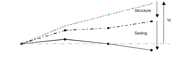
Figure 2.2 illustrates these volume, structure and saving effects.
Volume effect
Society shows a continuous increase of activities in various areas that often require extra energy. The extent of socio-economic activities is usually described by:
• gross domestic product (GDP) on a national level, • value added or production volume in production sectors, • total inland expenditure in households,
• transport performance in transportation.
These quantities are called ‘volume quantities’ here. If the volume of socio-economic activities grows, but all other factors remain unchanged, then the energy consumption will increase in
ac-cordance with the growth of the volume variable. On a national level, for example, this means that the total energy consumption increases with the same speed as GDP. The energy consump-tion development according to the socio-economic volume quantities is called ‘volume energy consumption’ in the protocol (see Figure 2.2).
Base year Reference year
Consumption Reference consumption Volume Saving Structure
Volume
Figure 2.2 Energy consumption developments and volume, structure and saving effect
The volume effect is equal to the increase of the volume energy consumption compared to the energy consumption level in the base year. It is assumed here that the energy consumption in-creases proportional to the increase of the volume of the activity.
Structure effect
As described earlier, the development of the reference consumption is linked directly to the trend for an energy-relevant variable. This trend is not only influenced by volume develop-ments, but also by various changes in the nature of the production and energy consumption that influence energy consumption (see Chapter 4 for examples per sector). The reference consump-tion usually develops along a different path than the volume energy consumpconsump-tion. This differ-ence can be ascribed to changes in the structure of productive and consumptive activities and is called the ‘structure effect’. The structure effect presented equals the difference between the ref-erence consumption and the volume energy consumption in the end year. In Figure 2.2 the structure effect slows down energy consumption trends as the reference consumption increases less than the volume energy consumption. The structure effect can also have an energy con-sumption promoting character.
Saving effect
As described earlier, the saving effect equals the difference between reference consumption and observed energy consumption in the end year. Taken together, the volume, structure and saving effect account for the total change in realised energy consumption between base year and end year. Further explanation of the volume, structure and saving effect can be found in Chapter 4 and in the Protocol report (Boonekamp, 2001).
Energy intensity and specific energy consumption
In energy consumption analyses, the terms ‘energy intensity’ and ‘specific energy consumption’ are often used. The protocol method refers to the relation between energy consumption and
(volume of) economic activity as the energy intensity (expressed in MJ/€). The term specific en-ergy consumption is used here in cases where enen-ergy consumption is related to physical vari-ables (e.g. MJ/ton steel or MJ/vehicle-km).
By definition, the volume effect no longer plays a role in the development of the energy inten-sity; the change in energy intensity is due to saving- and structure effects. For that reason, a de-crease in energy intensity cannot be called savings or improved energy efficiency.
2.3 Energy
consumption
quantities
The protocol method adheres as much as possible to the statistical information of Statistics Netherlands (CBS). The energy statistics are published annually in the Dutch NEH (Neder-landse Energie Huishouding). However, for the protocol choices have to be made on which data to use, and the data will have to be processed. These adaptations are done in the MONIT system and will be discussed below (Boonekamp, 1998).
Energy consumption sectors
In statistics the division of energy consumers is based on SBI codes (Standard Industrial Classi-fication of economic activities). In the Energy Balance format CBS distinguishes end user sec-tors (households, industry, transportation and other consumers) and energy secsec-tors (refineries, electricity generation and other energy companies). Transportation comprises both transport companies, own freight transport of other companies and passenger cars in households. The category other energy consumers consists of agriculture and horticulture, construction and ser-vices (trade, commercial serser-vices and public serser-vices). Other energy companies consist of gas supply, coke plants and distribution companies. In this recent analysis the sector definition has been slightly altered due to the new division that was agreed upon in the framework of the for-mulation of sectoral indicative targets for CO2 emissions (See Annex A).
In 1994 a new sector, decentralized (co-)generation of electricity, was introduced in the energy statistics of CBS. This sector involves mainly cogeneration plants that are administered by more than one party, e.g. an industrial company and an energy distribution company (so-called joint ventures). In the protocol calculations the joint venture capacity is transferred to the industrial sectors where the plant is physically present.
Energy carriers
Energy consumption means consumption of energy carriers such as coal, coke, crude oil or oil products, residual gases, electricity and steam or hot water. The consumption of various energy carriers can be added up as the energy content for every energy carrier has been defined (e.g. 31,65 MJ per m3 natural gas). Energy carriers are often divided in primary energy carriers, such as crude oil, coal, uranium and natural gas, or secondary energy carriers such as motor fuels, electricity and heat. The energy companies transform primary energy carriers into secondary en-ergy carriers that can be used by enen-ergy consumers.
Energy use
CBS provides an energy use figure for all sectors that equals: • energy deliveries (+),
• own energy supply, among which renewable energy (+), • energy deliveries to other sectors (-).
This energy use is corrected - if necessary- for changes in the stock of energy carriers at the site of the energy consumers.
Total Primary Energy consumption (TPEC)
Energy use at the national level is the Total Primary Energy consumption (TPEC). This quantity is the sum of all energy extraction and import, minus export and changes in the stocks of energy carriers. Export also includes bunkering, i.e. fuels bunkered by international shipping and avia-tion. The TPEC also equals the sum of energy use of all end users and energy suppliers.
Non-energetic energy consumption
According to the NEH approximately 14% of total energy consumption in the Netherlands was used for ‘non-energetic purposes’ in 1995. This is mainly the case in the chemical industry, where this energy consumption is usually referred to as ‘feedstocks’. In international analyses (e.g. IEA) the so-called ‘non-energy use’ is often not included. In the protocol, however, this energy consumption is included, but as a separate part of total energy consumption. In this way statements can also be made about the energetic applications of energy carriers only.
Temperature-corrected energy use
The average outdoor temperature during the heating season influences the energy consumption for space heating. In the past this effect amounted to approximately 10% in some years (see Figure 4.14). This stochastic effect hampers the analysis of energy consumption trends in rela-tion to socio-economic trends and policy measures. Therefore the statistical energy consumprela-tion data are corrected for temperature. The part of the statistical energy consumption that is used for space heating is increased or decreased depending on the deviation of outdoor temperature from the 30-year average. The deviation is expressed in the number of degree days compared to the standard number of degree-days (3200 in the period 1960-1990). The largest corrections (in PJ) occur for gas consumption of dwellings and buildings, but heat deliveries from district heating systems show also substantial corrections.
Final energy consumption
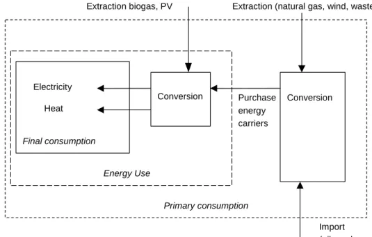
The relation between final energy consumption and energy use is illustrated in Figure 2.3. Pur-chased energy carriers are converted at the consumer into the so-called final energy carriers heat and electricity. In particular production with cogeneration plants causes a (small) conversion loss. As a result total final energy consumption of a sector is smaller than total energy use. More important however is the fact that final energy consumption has a different composition than energy use. For instance electricity use of the paper industry regards only half of final electricity consumption; the remainder is produced in own cogeneration plants. Thus energy use does not offer a correct view of the real energy consumption of electricity within the sector. Therefore the protocol uses final energy consumption to adequately specify the relation between energy consumption and the activities for which the energy was used.
Energy Use
Primary consumption
Extraction biogas, PV
Final consumption
Extraction (natural gas, wind, waste)
Purchase energy carriers Import (oil, coal, electricity) Heat Electricity Conversion Conversion
Figure 2.3 Relation energy use with final energy consumption and primary energy consumption
In addition, it appears in practice that the consumption and savings for final electricity consumption show a completely different pattern than final consumption of fuel/heat. This coheres with the very different applications of both energy carrier types. The same reasoning holds for non-energetic energy consumption. Thus, three nearly separated end use applications can be distinguished in the protocol method:
cks). • final electricity consumption, • final fuel/heat consumption,
• final non-energetic energy consumption.
The final electricity consumption is the sum of purchased electricity and own electricity produc-tion. In the transportation sector, the final fuel/heat consumption consists entirely of motor fuels. In other sectors, it is the sum of steam and hot water deliveries, own production of heat in co-generation plants and heat from conversion of final fuel consumption (fuel, not used for cogeneration or used as feedsto
Energy consumption in primary units
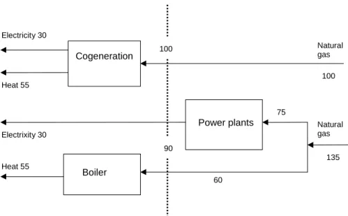
One adaptation of the statistical data that is necessary for the protocol involves the translation of energy use into energy consumption in primary units. Total energy use of a sector is the aggre-gate of all energy carriers on the basis of their energy content. The highest-quality energy carrier electricity can be used everywhere with a very high conversion efficiency. Therefore large-scale application of electricity appears to have a positive effect on energy use trends. However, in or-der to deliver the electricity, power plants are facing substantial conversion losses. To provide a true insight into the developments, the losses that occur elsewhere should be taken into account. The protocol therefore uses the quantity ‘energy consumption in primary units’ in end user sec-tors (see Figure 2.3). The energy consumption in primary units of an end user sector equals en-ergy use times a correction factor per enen-ergy carrier, representing the losses that occur else-where due to the delivery of this energy carrier to the sector (see also the end of this section). An important practical reason to use energy consumption in primary units is to unhide the sav-ing effect of combined cogeneration production. This is illustrated in Figure 2.4 where the same amounts of heat and electricity are produced via either cogeneration or power station/boiler
pro-duction. For cogeneration energy use is higher (100 to 90) but the energy consumption in pri-mary units is lower (100 to 135). Thus, energy consumption in pripri-mary units is needed to visual-ise the saving effect of cogeneration.
Cogeneration
Energy use Primary
Power plants Electricity 30 Electrixity30 Heat55 Heat55 Boiler Natural gas Natural gas 75 60 135 100 100 90
Figure 2.4 Energy use and energy consumption in primary units for cogeneration and separate
generation of heat and electricity
Static and dynamic energy consumption in primary units
The energy consumption in primary units in a certain year can be determined using multiplica-tion factors that apply to the year in quesmultiplica-tion. The development of this ‘dynamic energy con-sumption’ in primary units is the result of energy consumption developments on the one hand and changes in the energy sectors on the other hand. For example, the dynamic energy con-sumption in primary units for households will decrease when electricity generation becomes more efficient, even if household will continue to consume the same amount of electricity. The energy consumption in primary units can also be determined with fixed multiplication fac-tors that apply to the base year: the so-called ‘static energy consumption in primary units’. The development of this energy consumption variable is only influenced by developments at the end user. The static energy consumption in primary units provides a more transparent view of en-ergy consumption trends for end users. In the protocol all enen-ergy consumption figures of the end use sectors are defined in primary units with fixed multiplication factors.
Multiplication factors
The multiplication factors that were used in the protocol indicate the conversion losses in the energy sectors. These factors are specified per type of energy carrier for a fixed base year (see Table 4.1). For the Dutch electricity supply the overall conversion efficiency (including grid losses) lies beneath 40%. This means that approximately 2.7 PJ fuel is needed to generate 1 PJ of electricity, or a multiplication factor of approximately 2.7. For oil products, the multiplication factor amounts to 1.05-1.10 and for natural gas to approximately 1.01. Grid supplied heat has a factor lower than 1, because less than 1 PJ extra fuel is needed to generate 1 PJ of heat from a power plant (see Table 4.1). In the calculation of the multiplication factor no distinction is made between energy consumer types; the value is based on the total deliveries of energy companies and is the same for all end users. The multiplication factors also apply to energy carriers that are used for non-energetic applications.
2.4
Calculation of savings per sector and national
In line with the preceding starting points a calculation scheme has been set up to actually calcu-late the energy savings. A condensed description of the scheme is given.
Sectors distinguished
The protocol distinguishes the following sectors3: • Households
• Industry (including Construction) • Agriculture and horticulture • Services
• Transportation • Refineries • Electricity supply • Other energy companies.
Where necessary for the analysis the sectors will be split up further but the results are only pre-sented at sector and national level.
The protocol method determines figures on savings for:
• final energy consumption in 5 end user sectors and refineries,
• conversion in the same sectors (cogeneration production and heat delivery), • conversion in electricity supply (more efficient plants and cogeneration).
Savings on final energy consumption
Final energy consumption per sector is divided into a number of applications with their own ERG (energy relevant variable). For each application the trend in the ERG is used to compose time series for the reference consumption. These figures per application are aggregated to sector level and compared to the figures for realised final energy consumption. The difference consti-tutes the savings on final energy consumption. As described earlier all energy consumption data are in static primary energy units. The savings on final energy consumption are also expressed in PJprimary.
Savings from cogeneration
Savings by means of more efficient conversion at end users mainly involve cogeneration pro-duction. The savings are calculated by comparing the cogeneration input with the total input for separate heat and electricity production. The reference system for heat is a gas fuelled boiler with a sector-specific conversion efficiency. The reference system for electricity is central elec-tricity production with its average conversion efficiency. The savings are calculated in PJ, both for the base year and the year of analysis. The increase in savings between both years is taken as the savings achieved with cogeneration.
Grid supplied heat to end use sectors also contributes to the savings of more efficient conver-sion, because this heat generally originates from cogeneration by electricity companies. The amount of savings is calculated by converting delivered heat into primary units and comparing this figure with the fuel consumption in case of own heat production. For grid supplied heat multiplication factor of only 0.5 is used (see also Section 2.3). As own heat production demands more than 1 unit of fuel per unit of heat grid supplied heat will lead to savings for the end use sector.
3
Savings in electricity production
The savings of energy companies regard refineries and electricity production. The savings of refineries are calculated in a similar manner as in industry. The conversion losses of power plants are calculated per type of plant (coal, waste combustion, nuclear and gas). This is done both for the actual efficiencies and for the base year efficiencies. The differences per type of plant are aggregated, resulting in total savings (in PJ) for power plants. This approach forestalls shifts in fuel mix influencing the savings. The savings of extra cogeneration by electricity com-panies are calculated in the same manner as with cogeneration of end users.
Sectoral and national savings
The savings (in PJ) of final energy consumption and cogeneration are added to determine total sectoral savings. Aggregate sector savings and that of power plants constitute national savings. Linking this result to the TPEC finally results in the national savings percentage.
Uncertainty analysis
All input data are subject to an uncertainty margin. In addition, a margin is ascribed to the rela-tionship between ERG and the reference consumption. This margin indicates how well the ERG trend ‘predicts’ energy consumption in case of no savings. Using a Monte-Carlo algorithm, the margins in the inputs are translated into a margin in the calculated saving results. Because of the so-called ‘law of the large numbers’ the margin in the national saving figure is smaller than the margin for the sectors. The margins are also smaller as the length of the period increases (see Gijsen, 2003). Due to the relatively large uncertainty, especially in the data of the most recent year, the protocol method uses average values that include the previous two years. This also de-creases the uncertainty margin.
3.
ENERGY SAVINGS 1995 - 2002
3.1
Calculation method and input data
The method applied here to calculate savings in conformity with the protocol energy savings has been described in the previous chapter. In this report 1995 is used as the base year; in previous analyses 1990 was used as the base year (Boonekamp, 2002; Vreuls, 2003). One reason to change the base year was the need for a new approach in industry, which demanded data that were not available for previous years (see Chapter 4). The change in base year was seized as an opportunity to apply minor changes in the determination of savings in other sectors as well. All energy consumption data used are retrieved from the MONIT system of ECN (Boonekamp, 1998) that relies heavy on CBS energy statistics. In MONIT the CBS data are corrected for yearly variations in outdoor temperature; moreover industrial cogeneration production is trans-ferred from decentralized production to industry. Also determined are final end use and the mul-tiplication factors (see Chapter 2) that are needed in the analysis of savings. The socio-economic and physical data needed have been taken from various sources (see Chapter 4).
3.2
Savings per sector and national
The savings as of 20024 are determined as an average for the period 1995-2002, distinguishing between:
• end use sectors: households, industry5
, agriculture/horticulture, services and transportation6, • energy sectors: refineries and electricity supply,
• the national level (see Table 3.1).
For end use sectors and refineries both the savings on final energy consumption and the effect of more efficient conversion (cogeneration production and heat deliveries) have been determined. The savings in the electricity sector are displayed under ‘national’. Total national savings turn out to amount to 1% per year; per sector the annual savings vary between 0.4 and 1.7%. The contribution of more efficient conversion amounts to approximately 0.2 to 0.6% for the relevant sectors.
Table 3.1 Saving results for the period 1995-2002
[mean % per year] National Industry Services Households Agriculture Transport Refineries Final consumption -0.7 -0.8 0.0 -1.2 -1.1 -0.4 -0.8 Cogeneration end users -0.2 -0.2 -0.5 0.0 -0.6 0.0 -0.2
Power station -0.1
Cogeneration energy sector 0.0 Total -1.0 -1.0 -0.5 -1.2 -1.7 -0.4 -1.0
The determination of savings in each sector is explained in Chapter 4. The following remarks on the results can already be made:
• For Services it was impossible to determine a figure for savings in final energy consump-tion. A suitable variable to calculate the reference consumption was not available and the energy consumption data were unreliable (see also Chapter 3.3). There is no reason to
4
The energy consumption data for 2002 have been averaged with that of the previous two years before the results were determined
5
Including construction, coke plants and decentralized cogeneration production.
6
sume that dissavings have occurred given the realisation of low energy new buildings. However, savings cannot be proved either. The final savings have been set at nil for practi-cal reasons, as the national savings figure is not influenced by an (unreliable) negative fig-ure for Services. The cogeneration savings for Services have been determined, though. • In industry, the figure on savings is related to total energy consumption including
feed-stocks. This figure is not directly comparable to that from the LTA evaluations (based on consumption for energetic purposes only).
• Cogeneration savings for Services and Agriculture include also savings due to grid-supplied heat (from cogeneration elsewhere). Cogeneration in industry includes both own production and joint-venture (decentralized) production.
3.3
Volume, structure and saving effects
In Figure 3.1 the actual change in national energy consumption is divided into so-called volume, structure and saving effects. At the national level the volume effect is the (hypothetical) increase in total energy consumption in conformity with the growth of GDP. At the sectoral level an en-ergy consumption trend can be determined on the basis of the volume development per sector: growth of value added in industry, growth of number of households in the domestic sector, growth of haulage in the transportation sector, etcetera. Together this results in a smaller growth of total energy consumption. This difference is represented by the main structure effect. Within the sectors all kind of changes (not savings) are taking place that affect energy consumption. This structure effect is sometimes positive, i.e. more electrical appliances per household, and sometimes negative, i.e. a more energy-extensive production structure in industry. Over all sec-tors the structure effect leads to relatively larger energy consumption (see Figure 3.1). Finally a number of saving effects are shown. The sum of saving, structure and volume effects delivers by definition the mutation in energy consumption.
0.0% 10% 2.0% 3.0% 4.0% GD P ef fect mai n st ruct ure effe ct stru ctur e ef fect savi ng e ffect end use coge nera tion savi ng e nd u sers savi ng e ffect e-s ecto r coge nera tion savi ng e -sec tor mut atio n co nsum ptio n 0.0% 10% 2.0% 3.0% 4.0% GD P ef fect mai n st ruct ure effe ct stru ctur e ef fect savi ng e ffect end use coge nera tion savi ng e nd u sers savi ng e ffect e-s ecto r coge nera tion savi ng e -sec tor mut atio n co nsum ptio n
Figure 3.1 Decomposition of change in national energy consumption 1995-2002
3.4 Uncertainty
margins in the results
In (Gijsen, 2004) the uncertainty margins for the savings figures have been analysed. The amount of uncertainty is determined by three factors:
• the error margin in the energy data for the base year and all analysed years, • the error margin in the value of the ERG (energy relevant variable)
The margins in all inputs have been translated into a margin for total savings per sector and na-tional savings, using a stochastic Monte Carlo simulation method The margin in the nana-tional savings figure for 2002 amounts to 0.3%-point; the margins for the different sectors are higher (see Annex C, table C.1). For Services the uncertainty was so high that is was impossible to pre-sent any figure on savings on final energy consumption. This uncertainty was due to a lack of suitable ERG-quantities to determine the correct reference consumption and the bad quality of the energy consumption data.
3.5
Trend in development of savings
Table 3.2 provides the national savings data for various periods as of 1995. From these data it can be concluded that the rate of savings is gradually decreasing, both for final energy consump-tion and for cogeneraconsump-tion and power plants.
When drawing conclusions one should take into account on the one hand the rather large uncer-tainty margins in the results, especially for final energy consumption. On the other hand, it should be noted that this trend appears in various sectors and is also supported by supplemen-tary analyses (see Chapter 4).
Table 3.2 Trend in national savings as of 1995
[mean % per year] 1995-2000 1995-2001 1995-2002
Final energy consumption 0.8 0.8 0.7
Cogeneration and power plants 0.4 0.3 0.3
4.
SECTORAL ENERGY CONSUMPTION AND SAVINGS TRENDS
4.1 Introduction
In this chapter the determination of the amount of savings per sector is explained into more de-tail. Also the underlying energy consumption developments per sector are analysed. This in-cludes, among others, the development of energy intensities over time and sector specific trends: stabilisation of electricity consumption in households, shifts in the sector structure in in-dustry, the influence of assimilation lighting in horticulture, etcetera. The analysis period is ex-tended to 1990-2002, as to put the energy developments in the general policy perspective since Kyoto.
Finally it must be noted that all energy consumption figures are corrected for yearly variations in mean outdoor temperature in the heating season, unless stated otherwise.
Used multiplication factors
As described earlier in Chapter 2, the protocol method uses energy consumption data in primary units. In this respect, the consumption of each energy carrier is multiplied by a specific multipli-cation factor. The multiplimultipli-cation factor is based on the conversion losses that occurred in base year 1995, in order to deliver the energy carrier to the end use sectors. Table 4.1 presents the multiplication factors for 1995 that were used in the protocol calculations. For the purpose of comparison the values of 2002 have been provided too.
Table 4.1 Used multiplication factors per energy carrier
Multiplication factors 1995 2002 Coal/coke 1,087 1,051 Oil products 1,070 1,080 Natural gas 1,012 1,018 Heat (delivered) 0.5 0.5 Electricity 2,746 2,689
Explanation of multiplication factors
The conversion losses of coke production determine the multiplication factor for coal and coke. The multiplication factor decreased after 1995, due to closing down one of the two production locations (see Section 4.9). The utilities energy consumption of refineries determines the multi-plication factor for oil products. That factor increased due to extra processing of crude oil be-cause of higher product quality demands (see Section 4.7). In gas supply natural gas - and re-cently also electricity - is used for compressors. The multiplication factor increases because more and more compression is needed as a result of decreasing pressure in the main gas fields. The multiplication factor for grid supplied heat is a value determined on the basis of an assess-ment of the extra PJ of fuel that are needed in electricity production to supply a PJ of heat. As this heat would otherwise have been dumped into the cooling water, this heat is partly ‘free of charge’, resulting in a multiplication factor of less than 1. The fuel input of power plants, insofar fuel is not ascribed to heat production, determines the multiplication factor for electricity. This multiplication factor also covers production in waste combustion plants and grid losses of dis-tribution companies (see Section 4.8).
4.2 Households
Development of savings according to protocol method
In the protocol method sectoral energy consumption is divided into different segments or appli-cations, each with its own ERG-quantity (see Chapter 2). For households the following applica-tions and ERG-variables apply:
• fuel and heat for space heating (number of households), • fuel and heat for hot tap water (number of inhabitants),
• electricity consumption for appliances and lighting (overall penetration degree). 7
Without savings each energy consumption segment is assumed to increase in conformity with the growth of the ERG-quantity specified. The aggregate of all applications, transferred to pri-mary energy units, constitutes the reference consumption. This energy consumption appears to increase faster than the total statistical energy consumption (corrected for temperature), meaning that savings are realised indeed. Table 4.2 shows the calculated savings expressed in a mean percentage per year. Because of uncertainties in the data for the last observed year an average value, including the previous two years, has been constructed. The savings on final energy con-sumption amount to 1.2% for the period 1995-2002. Since the end of the nineties, the savings appear to decrease slightly, from 1.4% to 1.2%.
Table 4.2 Development of savings for Households, according to the protocol method
[%/year] 1995-1999 1995-2000 1995-2001 1995-2002
Final energy consumption 1.4 1.2 - 1.3 1.1 - 1.2 1.2
Cogeneration and district heating 0.0 0.0 0.0 0.0
Total 1.4 1.2 - 1.3 1.1 - 1.2 1.2
Next to final energy consumption, other savings can be realised in the households sector through the application of district heating. The number of connections has increased with 50% as of 1990. The total heat delivery has barely increased though (according to statistics and cor-rected for temperature) because the heat consumption per household has decreased significantly. To the extent that this is the result of savings on heat demand, it is taken along in the saving fig-ure for final energy consumption. As no extra heat has been produced compared to 1995, nor any change in the production, no extra savings have been realised for district heating. As a con-sequence no savings can be ascribed to the households sector (see Table 4.2).
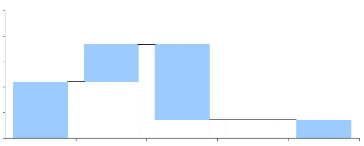
Volume, structure and saving effects
The limited increase of energy consumption in the households sector is the result of relatively large, yet opposing, effects (see Figure 4.1).
7
The overall penetration rate is an average of the increase of the penetration rates of all large households appliances, weighed for the electricity consumption per appliance.
0,0% 0,4% 0,8% 1,2% 1,6% 2,0%
volume-effect structuur-effect besparings-effect eindverbruik
wkk-besparing eindverbruikers
mutatie verbruik volume effect structure effect saving effect
end use
cogeneration saving end users
mutation consumption 2.0% 1.6% 1.2% 0.8% 0.4% 0.0%0,0% 0,4% 0,8% 1,2% 1,6% 2,0%
volume-effect structuur-effect besparings-effect eindverbruik
wkk-besparing eindverbruikers
mutatie verbruik volume effect structure effect saving effect
end use
cogeneration saving end users
mutation consumption 2.0% 1.6% 1.2% 0.8% 0.4% 0.0%
Figure 4.1 Volume, structure and saving effects for Households 1995-2002
The volume effect involves the energy consumption increase in conformity with the growth of the number of households. The structure effect entails:
• a faster increase in the number of dwellings compared to the number of households (appli-cation space heating),
• a decrease in the average size of households (application hot water consumption),
• an increase in the number of large household appliances per household (application electric-ity for appliances).
Together, these three structural trends lead to a larger energy consumption increase than could be expected on basis of the number of households; the structure effect comes on top of the vol-ume effect (see Figure 4.1). If the saving effects are taken into account too, the energy consump-tion increase amounts to only 0.3% per year.
Next to the above-mentioned factors other factors have also influenced energy consumption, among which:
• decreasing occupation of the dwelling (due to increased labour participation), • more intensive use of appliances,
• higher settings for space heating thermostat.
These factors are not part of the structure effect, though. Any possible effect on energy con-sumption of these factors will be part of the saving effect.
Background energy consumption developments in Households
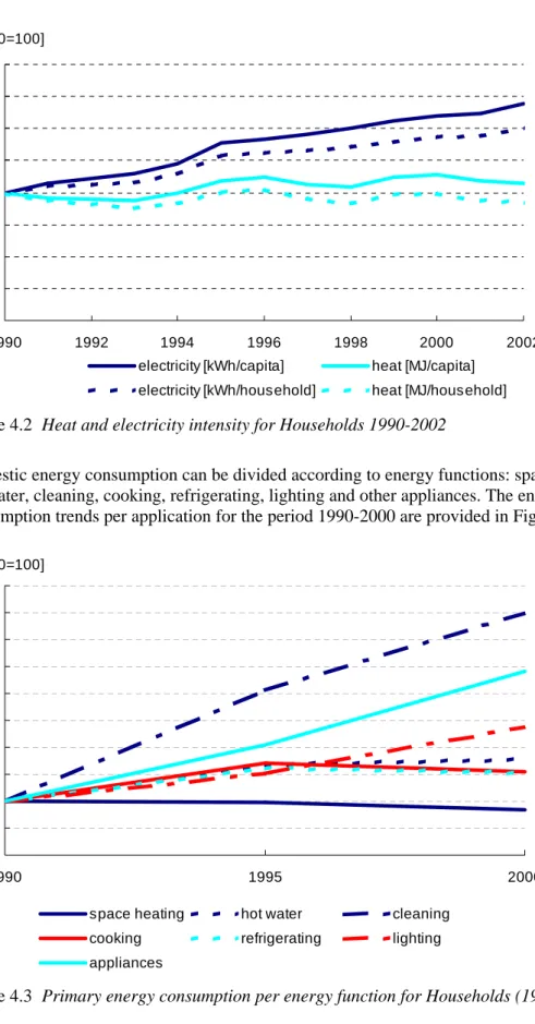
In the period 1990-2002 the number of inhabitants has increased with 0.6 to 0.7% per year and the number of households has increased with 1.2%. Household expenditures have increased on average with 2.8%. The increase in energy consumption (corrected for temperature) is very lim-ited, i.e. 460 to 467 PJ. There have been very few changes in the fuel mix over the last decades. Important fuels are gas, electricity and grid supplied heat. The electricity consumption increased with 38% in the period 1990-2002; gas consumption decreased with 2-3%; heat consumption increased strongly from 5.6 to 7.7 PJ, but the share remained limited. Because the share of elec-tricity consumption increases from 13% to 18%, primary energy consumption increases more strongly than energy consumption itself, i.e. with 5%.
In Figure 4.2, the growth of final consumption of heat and electricity is compared to that of population and number of households. Contrary to the growth trend for electricity per household
the trend for heat shows almost stabilisation. It should be noted that the intensity of fuel con-sumption develops even more favourably, because the average boiler efficiency has increased.
60 70 80 90 100 110 120 130 140 1990 1992 1994 1996 1998 2000 2002 [1990=100]
electricity [kWh/capita] heat [MJ/capita] electricity [kWh/household] heat [MJ/household]
Figure 4.2 Heat and electricity intensity for Households 1990-2002
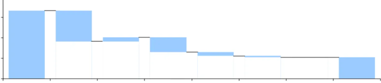
Domestic energy consumption can be divided according to energy functions: space heating, hot tap water, cleaning, cooking, refrigerating, lighting and other appliances. The energy
consumption trends per application for the period 1990-2000 are provided in Figure 4.3.
80 90 100 110 120 130 140 150 160 170 180 1990 1995 2000 [1990=100]
space heating hot water cleaning cooking refrigerating lighting appliances
Figure 4.3 Primary energy consumption per energy function for Households (1990=100)
For the sake of comparability electricity consumption has been converted into primary energy consumption. The trends per energy function are based on a separate analysis with the simula-tion model of historic household energy consumpsimula-tion (Boonekamp, 1997). The energy
con-sumption for space heating decreases a bit due to insulation, high efficiency boilers and more energy-efficient new dwellings. The energy consumption for cleaning increases the most, due to the penetration of the clothes dryer. The energy consumption of other appliances increases too as a result of a large increase in ownership of various appliances. However, since the energy consumption of these appliances is small, the total primary energy consumption increases only slightly.
The growth of expenditures, expressed in billion €, is often seen as an important cause for in-creasing energy consumption. Figure 4.3 demonstrates that this is mainly the case for energy functions where electricity consumption plays a role. Table 4.3 illustrates the relation with ex-penditures for different periods.
Table 4.3 Growth of expenditures and electricity consumption for Households
[%/year] 1990-1994 1994-1998 1998-2002 1990-2002
Expenditures 2.3 3.4 2.6 2.8
Expenditures per household 0.8 2.4 1.6 1.6
Final electricity 2.9 3.0 2.3 2.7
Final electricity per household 1.4 2.0 1.3 1.5
Electricity compared to expenditures +0.6 -0.4 -0.3 -0.1 Until 1994, electricity consumption appears to increase more rapidly than expenditures (intensity +0.6%, but with a larger income increase in the period 1994-1998 the electricity consumption increase lags behind (intensity -0.4%). This unlinking remains intact with a decreasing growth of expenditures after 1998. This could point to a structural saturation trend in which several electric appliances such as the dryer and dishwasher have reached their maximum penetration and no new ‘heavy’ energy consumption devices developing.
4.3
Industry (including construction)
Development of savings according to the protocol method
The energy consumption in construction and coke plants (4% and 1% of industrial energy con-sumption respectively) has also been ascribed to industry. That coheres with the definition of sectors used in the formulation of indicative targets for sectoral CO2 emissions.
To determine savings total industrial energy consumption is divided into the three applications electricity, fuel/heat and feedstock, as well as the following subsectors:
• food and beverages, • chemical industry, • iron and steel production, • non-ferro (aluminium, zinc), • paper and printing,
• building materials, • other metal, • other industry.
Neelis (2004) has determined the development of the reference consumption for the first six subsectors (i.e. excluding other metal and other industry). For these subsectors electricity and heat consumption in the base year is ascribed to a number of physical products. Energy con-sumption is scaled in conformity with the development of physical production8. The reference consumption for ‘other metal’ and ‘other industry’ is determined using the trend in sales in
stant prices. The total reference consumption thus determined, minus the statistical energy con-sumption, results in savings on final energy consumption.
Table 4.4 provides the calculated savings as an average from 1995 until the year in question. The savings on final energy consumption appear to decrease since 2000, namely from 1.0% to 0.8% per year. It should be noted that physical data for the year 2002 were not available in the food and chemical industry and non-ferro. Therefore the last year was partly based on estimates. However, this has only a limited effect on the margin for 2002 as the figures for 2002 have been averaged with that of the two previous years.
Table 4.4 Development of savings in Industryaccording to the protocol method
[%/year] 1995-2000 1995-2001 1995-2002
Final energy consumption 1.0 1.0 0.8
Cogeneration and heat delivery 0.1 - 0.2 0.1 - 0.2 0.2
Total 1.1 - 1.2 1.1 - 1.2 1.0
Note:Industry including Building industry and coke plants.
Next to final energy consumption, the application of cogeneration also leads to savings. Savings from cogeneration in industry originate from:
• own cogeneration production,
• decentralized (cogeneration) production in industrial companies,
• grid supplied heat from cogeneration production elsewhere (small contribution).
As can be seen in Table 4.4 cogeneration has delivered a substantial contribution to the total in-dustrial savings (see also the extended analysis of cogeneration savings in Chapter 5).
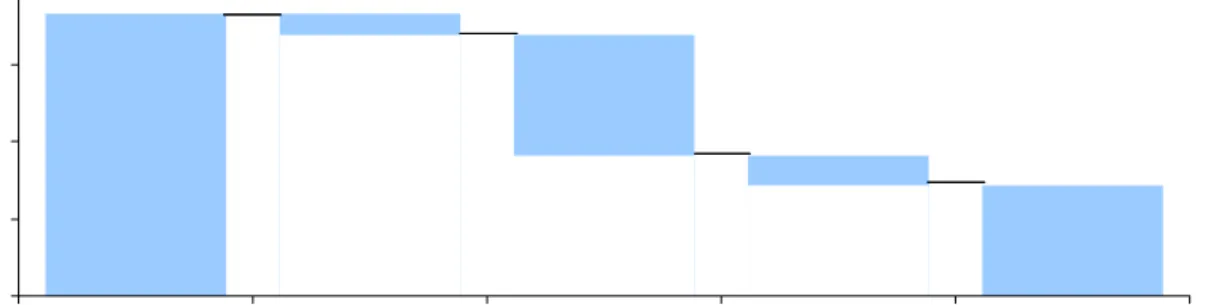
Volume, structure and saving effects
The increased energy consumption of industry is the result of relatively large, yet opposing, ef-fects (see Figure 4.4). The volume effect involves the energy consumption increase following the growth of total value added in industry. The structure effect involves:
• the shift between the shares of energy-intensive and energy-extensive subsectors in total value added,
• changes in the relation between the total value added and the physical production in the six subsectors analysed,
• changes in the relation between the total value added and the sales in constant prices (other metal and other industry).
0,0% 0,5% 1,0% 1,5% 2,0%
volume-effect structuur-effect besparings-effect eindverbruik
wkk-besparing eindverbruikers
mutatie verbruik
volume effect structure effect saving effect
end use
cogeneration saving end users
mutation consumption 2.0% 1.5% 1.0% 0.5% 0.0%0,0% 0,5% 1,0% 1,5% 2,0%
volume-effect structuur-effect besparings-effect eindverbruik
wkk-besparing eindverbruikers
mutatie verbruik
volume effect structure effect saving effect
end use
cogeneration saving end users
mutation consumption 2.0% 1.5% 1.0% 0.5% 0.0%
volume effect structure effect saving effect
end use
cogeneration saving end users
mutation consumption 2.0% 1.5% 1.0% 0.5% 0.0%
Together, these developments lead to a slightly smaller energy consumption increase than would have been the case according to the value added trend for industry; the structure effect compensates the volume effect for a small part (see Figure 4.4). When the different saving ef-fects are included, the energy consumption increase amounts to 0.7% per year.
Other factors than mentioned previously (excluding savings) influence energy consumption too. These are not part of the structure effect though. Some examples are:
• extra operations for physical bulk products (e.g. coating of steel), • extra measures due to safety regulations or environmental regulations,
• physical production trends in other metal and other industry that deviated from sales trends, • changes in the rate of capacity utilisation of energy intensive production processes.
The possible energy consumption effect of these factors is included in the saving effect.
Background energy consumption developments in industry
The analysis limits itself to the industry only, without the (relatively small) energy consumption of construction and coke plants. This facilitates the comparability of the results with that of other studies and data sources.
The total energy consumption in the period 1990-2002 varies between 960 and 1132 PJ (cor-rected for temperature). On balance the increase amounts to 17% (1.3%/year). Figure 4.5 shows that oil consumption is increasing the most, especially for use as feedstock (+4.6% per year). Electricity consumption decreases because more and more electricity comes from own genera-tion. As a result of the decreasing share of electricity, total energy consumption in primary units increases with 12% only.
0 100 200 300 400 500 600 1990 1992 1994 1996 1998 2000 2002 [PJ]
Kolen coal Olieproducten oil products Aardgas natural Warmte heat Elektriciteit electricity
Figure 4.5 Consumption per energy carrier in Industry 1990-2002 (excluding construction)
The industry is divided in subsectors food and beverages, base metal, chemicals, paper, other metal, building materials and other industry. The primary energy consumption of the chemical industry is by far the largest. Its fraction in industrial energy consumption is still increasing,
slightly decreased in 2002. The share of food and beverages increases from 9% to 10%; the share of building materials decreases relatively strongly (4.4% to 3.1%), as does the share of other industry (5.0% to 3.6%). The subsectors paper and other metal maintain their share (approximately 4% and 6% respectively).
In final energy demand three distinctive applications are distinguished: • heat production in boilers, furnaces, etcetera,
• electricity consumption,
• use of energy carriers as feedstocks.
Figure 4.6 shows the ratio of final energy demand to production, expressed in € value added. Final electricity demand, covered by cogeneration or the grid, increases nearly as fast as value added in the period 1990-2002 (1.7 and 1.8% per year respectively). From 1990 tot 2002 the feedstock energy consumption increases similarly to the value added. But this is the result of a remarkable trend break in the mid nineties. Final heat demand barely increases; the heat inten-sity decreases with 1.6% per year on average. But in this case too, a remarkable change in the trend is visible recently. It must be remarked that a recent investigation of CBS indicates that the observed shift in later years, from fuel use to feedstock use, has to be revised.
70 75 80 85 90 95 100 105 110 1990 1992 1994 1996 1998 2000 2002 [1990=100]
electricity [kWh/euro TW] heat [MJ/euro TW] feedstock [MJ/euro TW]
Figure 4.6 Electricity, heat and feedstock intensity for Industry 1990-2002
Table 4.5 describes the economic development of the most energy-intensive sectors and of total industry. It shows that the most energy-intensive part of industry, the chemical industry, grew faster than total industry in the period 1990-2002. In eight out of the twelve years in this period, the growth of chemicals exceeds that of total industry. Other energy-intensive subsectors, such as base metal and paper, grew slower than total industry. But all in all, the subsector develop-ments between 1990 and 2002 have led to a more energy-intensive production structure, espe-cially in the last four years.
Table 4.5 Annual growth rate value added of industry and energy-intensive subsectors 90-91 91-92 92-93 93-94 94-95 95-96 96-97 97-98 98-99 99-00 00-01 01-02 90-02 Industry 0.6 1.0 -1.7 6.8 3.2 0.4 3.5 3.0 3.0 3.9 -0.9 -1.2 1.8 Chemicals -3.7 -3.3 0.2 10.9 6.4 -3.7 5.3 -0.4 6.7 7.9 3.5 2.9 2.6 Base metal -3.3 -7.0 -2.5 9.6 1.1 -2.4 8.3 2.0 0.3 1.7 -1.3 -1.9 0.3 Paper 2.6 0.6 -0.1 4.3 0.8 1.8 4.4 5.8 1.4 1.9 -1.6 -3.1 1.5
Apart from shifts between subsectors other developments within the subsectors are also important for the relation between total production and total energy consumption. Figure 4.7 and 4.8 provide the trends for the most important sectors with regard to the electricity and heat intensity. For electricity, the intensities are always close to the level of 1990, except for the chemical industry since of 1998. For heat, a downward trend can be seen for all sectors, with the exception of base metal that first shows an increase from 1990 on. Here, the differences between the subsectors are larger than for electricity.
60 70 80 90 100 110 120 130 1990 1992 1994 1996 1998 2000 2002 [1990=100]
food base metal chemical ind. paper