Sensitivity of ozone concentrations in the LOTOS-EUROS model

(1)

Report 500045003/2005

Sensitivity of ozone concentrations in the LOTOS-EUROS model

F.P.E. Brouwer

Contact: G.J.M. Velders

Netherlands Environmental Assessment Agency (MNP) Guus.Velders@mnp.nl

Process Report Environmental Science nr. 18

This report is part of the Series Process Reports Environmental Science of the Department of Environmental Science of the Radboud University Nijmegen.

This investigation has been performed by order and for the account of the Ministry of Housing and Physical Planning, within the framework of project M500045, “Model Instruments Air”.

Netherlands Environmental Assessment Agency (MNP associated with the RIVM), P.O. Box 303, 3720 AH Bilthoven, the Netherlands, telephone: +31-30 274 274 5, website: www.mnp.nl

(2)

(3)

Abstract

Sensitivity of ozone concentrations in the LOTOS-EUROS model

The study reported here describes the influence on ozone concentrations in the LOTOS-EUROS model of model parameters, chemistry scheme, VOC emissions, NOx emissions,

convergence of the chemistry scheme, washout ratios in wet deposition, emission time profiles and the boundary conditions for ozone. The most important outcome of this study was that results were found to be highly dependent on the applied chemistry scheme, boundary ozone concentrations and NOx emissions and less dependent on the implemented

VOC split and washout ratios.

Keywords: troposphere, chemistry, Europe, boundary conditions, VOC-split

Rapport in het kort

Gevoeligheid van ozonconcentraties in het LOTOS-EUROS model

In dit rapport wordt beschreven de gevoeligheid van de ozonconcentraties in het LOTOS-EUROS model als gevolg van veranderingen in modelparameters, chemieschema, VOS emissies, NOx emissies, convergentie van het chemie schema, natte depositiesnelheden,

emissie tijdprofielen en de ozonrandvoorwaarden. Het belangrijkste resultaat is dat de resultaten sterk afhankelijk bleken te zijn van het toegepaste chemieschema, de ozonrandvoorwaarden en de NOx emissies en minder van de VOC-split en de natte

depositieparameters.

(4)

Preface

This study was carried out in the framework of my traineeship at MNP, forming part of the Masters’ degree programme in Environmental Sciences at the University of Nijmegen. I would like to thank Guus Velders, Ferd Sauter, Martijn Schaap and Mark Huijbregts for their guidance during this study.

(5)

Samenvatting

LOTOS en EUROS zijn beide Europese verspreidingsmodellen voor het modelleren van lucht vervuilende stoffen. LOTOS is afkomstig van TNO, EUROS is ontwikkeld bij het RIVM/MNP. Er is besloten samen te werken en deze modellen samen te voegen tot het LOTOS-EUROS model.

Om inzicht te krijgen in de werking van het nieuwe model is het nuttig te weten voor welke parameters het model gevoelig is. In dit project zijn enkele parameters gevarieerd en is het effect op de berekende ozon-concentraties bekeken. De conclusies die hieruit getrokken kunnen worden zijn:

- De resultaten worden significant beïnvloed door de keuze van het chemieschema (CBMIV of CB99).

- Resultaten zijn weinig gevoelig voor de samenstelling van de VOC-split, een verdubbeling van de VOC emissies heeft echter een significant effect.

- Veranderingen in NOx emissies hebben een groot effect, dit is niet lineair, maar hangt af

van de omstandigheden in het systeem. In de gemodelleerde periode kunnen NOx

gelimiteerde periodes onderscheiden worden.

- Een minimum aantal van 10 iteraties in de chemie-module lijkt optimaal te zijn omdat meer iteraties weinig effect hebben. Opvallend is het dat ozon-concentraties systematisch lijken af te nemen met een toenemend aantal iteraties.

- Uitwasconstanten in de natte depositiemodule hebben minder invloed op berekende ozon-concentraties dan verwacht.

- Het effect van dagelijkse, wekelijkse en jaarlijkse tijdsafhankelijkheid van de emissies in het model is klein. De aanwezigheid van tijdsprofielen geeft echter een net iets betere correlatiecoëfficiënt met de waarnemingen dan wanneer deze niet toegepast worden. - Het variëren van ozon-concentraties aan de grenzen van het systeem heeft grote invloed

op berekende ozon-concentraties binnen het systeem. Door deze grensconcentraties aan te passen, bijvoorbeeld door middel van een functie waarin bijvoorbeeld het aantal zonuren is opgenomen, zouden de resultaten mogelijk kunnen worden verbeterd.

- De chemieschema’s reageren niet hetzelfde op variatie in de parameters, CB99 lijkt gevoeliger dan CBMIV.

(7)

Summary

LOTOS and EUROS are chemical transport models for air pollutants on a European scale developed by TNO and RIVM/MNP, respectively, and later integrated into the LOTOS-EUROS model. Investigating the model’s sensitivity to different parameters was thought useful for gaining a better understanding of its features. This idea took form in my study aimed at investigating the influence of varying several parameters on calculated ozone concentrations. A number of conclusions drawn from this investigation are listed below. - Results are highly influenced by the choice of chemistry scheme (CBMIV or CB99). - Results are little influenced by the composition of the VOC-split; variation in the VOC

emissions, however, has a relatively large effect on ozone concentrations.

- NOx emissions have a significant, non-linear, effect on ozone concentrations, depending

on the circumstances in the system. During the modelling period, NOx-limited periods as

well as non-NOx limited periods could be observed.

- Ten iterations would seem the optimal value for the minimum number of iterations in the chemistry module, as more iterations only slightly influence model results. Striking is that ozone concentrations systematically decrease when the minimum number of iterations increase.

- Washout ratios in wet deposition have less influence on ozone concentrations than was expected.

- Although the influence of emission time profiles is only small, correlation coefficients are slightly better when the time dependency of emissions is implemented.

- Variation in boundary ozone concentrations has a major effect on calculated ozone concentrations. Adjusting these values, for example, by employing a function in which the hours of sunshine are included may improve results.

- CB99 and CBMIV responded differently to the variation among the parameters, with CB99 seemingly more sensitive to the varying parameters than CBMIV.

(8)

(9)

1. Introduction

TNO and RIVM separately developed chemical transport models for air pollutants on a European scale. These two models (LOTOS and EUROS respectively) have the same structure. It was decided to set up a cooperation in which the two models are integrated into the LOTOS-EUROS model (Schaap et al., 2005).

LOTOS-EUROS is, just as LOTOS and EUROS both are, a 3D Eulerian chemistry transport model. It describes transport of air pollutants by use of atmospheric chemistry and wet and dry deposition modules. Meteorological data is derived from ECMWF or from UBA Berlin. LOTOS-EUROS is developed in such a way that the chemistry schemes CBMIV (used in LOTOS) and CB99 (used in EUROS) can both be applied. These chemistry schemes use different groups of species, which has to be taken into account in the input files. Emissions of volatile organic compounds (VOC) are given in VOC-splits, in which the total VOC

emissions are divided into species per emission sector.

To get more insight into the new, combined model, it is useful to analyse its sensitivity towards different parameters. This report discusses the influence of the following parameters on calculated ozone concentrations:

- Chemistry scheme (Chapter 2) - VOC-split (Chapter 3)

- NOx emissions (Chapter 4)

- Iterations in chemistry module (Chapter 5) - Wash out ratios in wet deposition (Chapter 6) - Emission time profiles (Chapter 7)

- Boundary conditions for ozone (Chapter 8)

In Chapter 9 all results are compared on basis of the difference of their AOT40 to reference runs. Appendix 1 gives an overview of all runs used in this report.

(10)

(11)

2. Chemistry schemes

In LOTOS-EUROS two chemistry schemes can be applied, namely: CBMIV and CB99. These are both carbon bond 4 mechanisms, CB99 is an updated version of the CBMIV mechanism. For more information about these mechanisms see Hammingh et al. (2001). Application of the different chemistry schemes does significantly affect ozone

concentrations.

In the Netherlands, day time peak values for ozone modeled with CBMIV are higher than that modeled with CB99. CBMIV values are in better agreement with observations during periods with high ozone concentrations. However, after smog events they are too high and the CB99 values are, although still too high, in better agreement with the observations. As can be seen from Figures 2.1 and 2.2, performance of the chemistry schemes highly depends on the modeled period and area.

Figure 2.1: Difference between CBMIV (run 929) and CB99 (run 932). Left: July, 31 1999 at 17:00. Right: August, 03 1999 at 07:00.

CB99 is 2 to 3 times more time consuming than CBMIV.

Comparison of calculation rates is however not straightforward. Because of different calculation methods, it is unclear what the threshold value for ongoing iterations is. To make proper comparison more information about these mechanisms has to be obtained. More info is included in Appendix 2.

Figure 2.2: Hourly mean ozone concentrations averaged over 22 background stations in the Netherlands, comparing CBMIV and CB99 chemistry for Jul/Aug 1999.

(12)

(13)

3. VOC-splits

Volatile Organic Compounds (VOCs) play a crucial role in atmospheric chemistry and in the formation and degradation of ozone. Therefore proper treatment of these compounds is very important. Many different types of VOCs are emitted into the atmosphere, each with its own reactivity and ozone forming potential. The differences between species cannot be neglected, as for example, encouragement of the use of less reactive VOCs could provide a cost

effective control strategy to achieve ozone reductions (Carter, 1994).

Model input is a bulk VOC emission, which is divided into emissions per species. This subdivision depends on emission category (e.g. transport, solvent use, etc.) and on the applied chemistry scheme. The composition of a VOC mixture is obtained from emission inventories.

3.1 Existing VOC-splits and deduction of new ones

Several VOC-splits are present at TNO and MNP, these are:

1. Euros CB99 (so far used in CB99) (Barrett and Berge, 1996) 2. Euros CBMIV (Barrett and Berge, 1996)

3. Lotos CBMIV (so far used in CBMIV) (Builtjes et al., 2003) 4. Trotrep CBMIV (Roemer et al., 2003)

These VOC-splits have different categories, species and units, which can be converted into each other.

VOC-splits 1 and 2 have 6 categories, namely: Combustion Domestic Refinery Industry Solvent Transport

The VOC-split currently used in CBMIV (3) has 12 categories, these are only numbered 1 to 12, no category names are provided.

The model works with SNAP codes instead of categories. LOTOS-EUROS assigns these codes according to the classification in Table 3.1.

When necessary the input VOC-splits are adjusted to the SNAP codes. The program code is adapted in such a way that it reads SNAP codes instead of the earlier used categories.

(14)

Table 3.1: Assignment of categories to SNAP codes in LOTOS-EUROS SNAP

code

SNAP name Category

(Euros/CB99, Euros/CBMIV)

Category (Lotos/CBMIV)

1 Power generation Combustion 1

2 Residential, commercial and other combustion

Combustion 1

3 Industrial combustion Combustion 1

4 Industrial processes Industry 4

5 Extraction, distribution of fossil fuels

Combustion 1

6 Solvent use Solvent 5

71 Road transport gasoline Transport 6

72 Road transport diesel Transport 7

73 Road transport lpg Transport 7

74 Road transport evaporation Transport 3

8 Other mobile sources Combustion 1

9 Waste treatment and disposal Combustion 1

10 Agriculture Combustion 1

To make the VOC-splits suitable as input files for the model, CBMIV must contain the species:

OLE (olefins)

PAR (paraffinic compounds) TOL (toluene) XYL (xylene) FORM (formaldehyde) ALD (aldehydes) KET (ketones) ACET (acetone) ETH (ethane)

UNR (unreactive compounds) For CB99 the chemistry scheme contains:

OLE PAR XYL FORM ETH ETOH (ethanol) MEOH (methanol) ALD2

The trotrep VOC-split has CBMIV species, to obtain an additional CB99 VOC-split, this scheme can be converted. To do this the chemical groups TOL, ACET and KET have to disappear and MEOH and ETOH have to be added (ALD becomes ALD2, values are kept the same, because the difference between these species is unclear, but assumed to be very little). In LOTOS-EUROS PAR, ACET and KET are not treated separately:

(15)

PAR’ = PAR + 3 ACET + 4 KET

In this way ACET and KET get incorporated in PAR. TOL is incorporated in XYL by simply adding TOL to XYL.

According to Barrett and Berge (1996) ETOH is incorporated in ALD in the CBMIV split. As Euros CBMIV and CB99 are derived from the same data, the ratio ALD:ETOH can be

deduced from these files and used to divide ALD into ALD’ and ETOH.

ETOHtrotrep, CB99 = ETOHEuros, CB99 * ALDtrotrep, CBMIV / ALDEuros, CBMIV

ALDtrotrep, CB99 = ALDtrotrep, CBMIV – ETOHtrotrep, CB99

Barret and Berge (1996) reported that MEOH makes 0.39 weight% of the total VOC emissions. In CBMIV MEOH is incorporated in PAR, it can therefore be calculated and subtracted from PAR. This different allocation has however, no significant influence on ozone concentrations (Appendix 3).

Input values for the LOTOS-EUROS model have to be in mol/kg VOC. Euros CBMIV is given in mass fractions. These can be converted by dividing them by the molar mass (kg/mol), which gives the desired units.

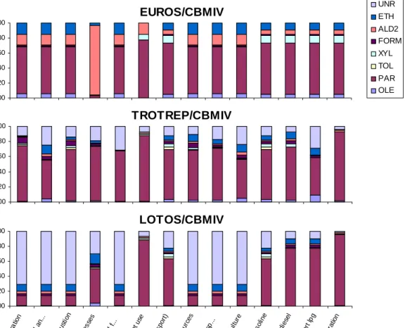
Figure 3.1 and 3.2 give the composition of the different VOC-splits per category.

Figure 3.1: Composition of VOC’s per category in CB99.

EUROS/CB99 0.00 0.20 0.40 0.60 0.80 1.00 Po we r g en era tion Re sid enti al, c om me rci.. Ind ustr ial com bu stio n Ind us tria l p roce sse s Ex tra ctio n d istr ibu tion .. So lve nt u se (Ro ad tr ans port) Oth er mo bile so urc es Wa ste tre atm ent a nd ... Ag ricu lture Ro ad tra nsp ort ga so line Ro ad tra nsp ort d iese l Ro ad tr ans port lpg Ro ad tr ans port ev apo r... Fr a c ti on ETOH MEOH UNR ETH ALD2 FORM XYL TOL PAR OLE TROTREP/CB99 0.00 0.20 0.40 0.60 0.80 1.00 Po we r ge ne ratio n Re sid entia l, c om me rci.. Ind ustr ial c om bust ion Ind ustr ial pro ces ses Ex tra ctio n d istr ibu tio.. . So lve nt u se (Ro ad tra nsp ort ) Oth er mo bile so urc es Wa ste tre atm en t an d... Ag ricu lture Ro ad tr ans port ga so... Ro ad tr ans po rt d iese l Ro ad t ran sp ort lpg Ro ad tr ans port ev a... Snaps F ract io n

(16)

Figure 3.2: Composition of VOC’s per category in CBMIV

3.2 Results for different VOC-splits

For several periods, model runs were performed to get information about the influence of different compositions of the VOC mixture. It can be concluded that differences in the implemented VOC-splits, only slightly influence ozone concentrations (Appendix 3). Correlation coefficients are the same for the different VOC-splits, this may however be different for other periods and areas.

To get information about the influence of individual species, emissions of each of the species in the trotrep split was decreased by 50%. Results are compared to the original VOC-split. Especially in CBMIV, decreasing individual species has little influence on the calculated ozone concentrations (Appendix 3). In CB99, effects are larger, but still limited. As reductions are a percentage of the emissions, instead of absolute amounts, no ranking in reactivity of the species, can be deduced from the results in Figure A3.4. To get insight in this reactivity, AOT40 is scaled by the relative VOC emission factor (mol/kg VOC) of an

individual species in Figure A3.5.

EUROS/CBMIV 0.00 0.20 0.40 0.60 0.80 1.00 Po we r g en era tion Re sid enti al, c om me rcia l an ... Ind ustr ial com bu stio n Ind ustr ial p roce sse s Ex tra ctio n d istr ibu tion of f... So lve nt u se (R oad tra nsp ort ) Oth er mo bile so urc es Wa ste tre atm ent and dis p.. . Ag ricu lture Ro ad tra nsp ort gas olin e Ro ad tra nsp ort die sel Ro ad t ran spo rt lp g Ro ad tr ans port eva pora tion F ract io n UNR ETH ALD2 FORM XYL TOL PAR OLE TROTREP/CBMIV 0.00 0.20 0.40 0.60 0.80 1.00 Po we r ge nera tion Re sid enti al, c om me rcia l an ... Ind ustr ial com busti on Ind ustr ial pro ces ses Ex tra ctio n d istr ibu tion of f ... So lve nt u se (R oad tra nsp ort) Oth er m obile so urc es Wa ste tre atm ent and dis p.. . Ag ricu lture Ro ad tr ans po rt g aso line Ro ad t ran spo rt d iese l Ro ad tr ans port lpg Ro ad tra nsp ort ev apo ratio n F ract io n LOTOS/CBMIV 0.00 0.20 0.40 0.60 0.80 1.00 Po we r g en era tion Re sid entia l, c om me rcia l an ... Ind ustr ial com bu stio n Ind ustr ial p roce sse s Ex tra ctio n d istr ibu tion of f... So lve nt u se (R oad tra nsp ort) Oth er mo bile so urc es Wa ste tre atm ent and dis p.. . Ag ricu lture Ro ad tr an spo rt g aso line Ro ad tra nsp ort die sel Ro ad tr ans port l pg Ro ad t ran sp ort ev apo ratio n Snaps p a rt p e r s p e c ie

(17)

As ozone chemistry is not a linear process, increasing concentrations may give other results than decreasing them. Therefore, ozone concentrations are calculated with an emission increase of 50% for each of the species as well. It can again be concluded that the influence of changes in the VOC-split is very little, especially in CBMIV.

A reason for the small influence of VOC emissions can be low concentrations of NOx. In

such a situation, ozone formation can be NOx limited.

Figure 3.3 shows differences in ozone concentrations when VOC emissions are doubled or halved. These differences are, as expected, more significant than effects of variations in the composition of the VOC-splits. Increasing VOC emissions result in increased ozone

concentrations, where decreased emissions give decreased ozone concentrations.

Notwithstanding the differences in the calculated ozone concentrations, from CBMIV and CB99, response on variation in VOC emissions is in the same order of magnitude for both chemistry schemes.

Figure 3.3: Upper left: Difference between ozone concentrations resulting from the original VOC emissions (Run 926) minus concentrations from the doubled emissions (Run 974) in CBMIV. Upper right: Difference between ozone concentrations resulting from the original VOC emissions (Run 926) minus concentrations from the halved emissions (Run 975) in CBMIV. Lower left: Difference between ozone concentrations resulting from the original VOC emissions (Run 931) minus concentrations from the doubled emissions (Run 978) in CB99. Lower right: Difference between ozone concentrations resulting from the original VOC emissions (Run 931) minus concentrations from the halved emissions (Run 979) in CB99.

(18)

(19)

4. NO

x

emissions

To get a picture of the role of NOx in the model, calculations are performed with NOx

emissions decreased or increased by 50%. As NOx is an important ozone precursor, the effect

of varying these emissions could be large. Ozone is produced by reactions 4.1-4.6 (Wayne, 1991). NO2 + hν Æ O + NO (4.1) O + O2 + M Æ O3+ M (4.2) OH + CO Æ H + CO2 (4.3) H + O2 + M Æ HO2+ M (4.4) HO2 + NO Æ OH + NO2 (4.5) CO + 2O2 + hν Æ CO2 + O3 (4.6)

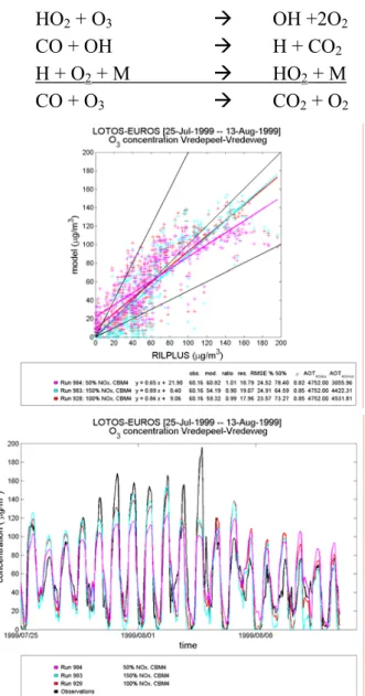
When however, not enough NO is present reaction 4.5 cannot proceed and reactions 4.7-4.10 take over, reducing ozone concentrations (Wayne, 1991).

HO2 + O3 Æ OH +2O2 (4.7)

CO + OH Æ H + CO2 (4.8)

H + O2 + M Æ HO2 + M (4.9)

CO + O3 Æ CO2 + O2 (4.10)

In such a case there is a NOx limited

situation, in which variations in VOC emissions will only slightly influence ozone concentrations.

Figure 4.1 shows results of variation of the NOx emissions by plus and minus

50%.

During the first nine days of the modeled period, increased NOx

emissions result in higher ozone concentrations, were decreased NOx

emissions give lower ozone

concentrations. This suggests a NOx

limited system, with ozone formation proportional to NOx concentrations. In

the latter part of the modeled period, this proportionality disappears and during the last three days it is even the other way around (increasing ozone concentrations with decreasing NOx

Figure 4.1: Influence of varying NOx emissions

by +/-50% on ozone concentrations at Vredepeel.

(20)

concentrations). This is caused by high NOx concentrations, which react directly with OH

(reaction 4.11), preventing ozone formation. Because there is still photolysis of ozone, ozone concentrations decrease with increasing NOx concentrations.

Appendix 4 shows NO2 concentrations during the modeled period.

OH + NO2 Æ HNO3 (4.11)

When enough NOx is present, hydrocarbons become the limiting factor in ozone production.

As can be seen in Figure 4.2, variation of the VOC emissions does not influence ozone concentrations during the first 4 days (25-28 July), as expected in a NOx limited system.

From day 5 till the end of the period ozone concentrations depend on VOC as well as on NOx

concentrations.

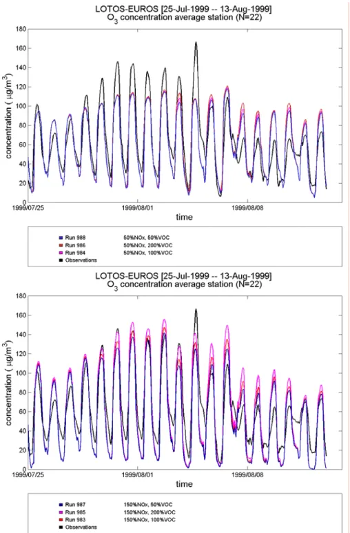
The modeled NOx or VOC dependence of ozone concentrations is shown in Figure 4.3, in

which NOx and VOC concentrations are varied simultaneously. It shows the minor influence

of VOC emissions when NOx concentrations are low. The response of ozone concentrations

to VOC emissions increases, when NOx emissions are increased.

Figure 4.2: Influence of varying VOC emissions by +100 and -50% on the ozone concentrations at Vredepeel.

(21)

Figure 4.3: Influence of simultaneous variation of NOx and VOC

emissions on ozone concentrations averaged over 22 background stations in the Netherlands.

(22)

(23)

5. Minimum number of iterations

For CBMIV chemistry, minimum and maximum number of iterations are specified in the input file. The length and output of model runs depends on the minimum number of iterations. It is taken 5, 10 and 15, to investigate its influence.

It can be concluded that 10 iterations seems to be sufficient. Increasing the minimum number of iterations hardly effects ozone concentrations, as can be seen in Figure 5.1. Striking however, is that ozone concentrations decrease with an increasing number of iterations. The calculation rate is only little influenced by the minimum number of iterations. Doubling the number from 5 to 10 iterations takes only 8% more CPU time (250 vs 269 min.).

Increasing the number of iterations from 5 to 15, increases the CPU time by 31% (250 vs 327 min.).

Correlation coefficients are the same for all three of the runs. For more information see Appendix 5.

Figure 5.1: Difference in ozone concentrations for runs with 5, 10 and 15 minimum iterations on 1999-08-11, 15:00 h. Upper left: 5 (Run 901) vs 10 (Run 904) iterations. Upper right: 10 (Run 904) vs 15 (Run 905) iterations. Bottom: 5 (Run 901) vs 15 (Run 905) iterations.

(24)

(25)

6. Washout ratios in wet deposition

Sudden decrease in ozone concentrations is poorly modeled by LOTOS-EUROS. Reason for such a sudden decrease in the observed ozone concentrations, can be a period of rain, as is in agreement with the meteorological data (Figure 6.1).

Wet deposition is partly controlled by washout ratios. The model version used so far, only includes washout ratios for SO2, HNO3, H2O2,

NH3 and formaldehyde

(FORM). In a new version of the model (0.4_001 and 0.4_002 for CBMIV and CB99, respectively) washout ratios for an extended list of species are included

(Appendix 6).

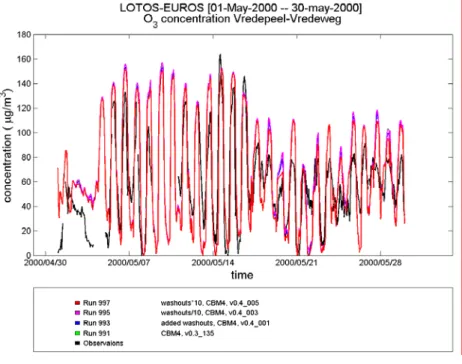
To investigate sensitivity to the washout ratios, these were divided and multiplied by 10. Ozone concentrations are highest when washout ratios are low and wet deposition is minimal.

Figure 6.2 shows that ozone concentrations are rather insensitive to the washout ratios, a factor 10 only slightly influences concentrations in periods of rain. However, because of great uncertainties, a factor 10 is not unrealistic.

A more direct effect of increasing and decreasing the washout ratios can be seen from other species than ozone. HNO3 and OH have high washout ratios (1.0*106 and 2.0*104,

respectively), therefore, periods of rain should have major effect on their concentrations in the atmosphere.

Figure 6.3 shows the effects of multiplying and dividing the washout ratios by a factor 10 on HNO3 concentrations. Although washout ratios do not have much effect, HNO3

concentrations decrease when washout ratios are increased and vice versa, which becomes especially clear during periods of rain.

(26)

Figure 6.2: Effect of variation in the washout ratios on ozone concentrations at Vredepeel, for May 2000, for CBM4 (top) and CB99 (bottom).

OH is not taken into account in earlier versions of the model, its washout ratio is added in the new version of the model. Figure 6.4 shows the influence of the washout ratios on calculated OH concentrations. The influence of variation in the washout ratios is obvious. However, the influence is less directly than it is for HNO3. A possible explanation for this can be the

(27)

Figure 6.3: Influence of washout ratios on HNO3 concentrations

at Vredepeel, for May 2000, for CBMIV

Figure 6.4: Influence of washout ratios on OH concentrations at Vredepeel, for May 2000, for CBMIV

The correlation coefficient (for data from Vredepeel) is, in CBMIV as well as in CB99, best when washout ratios are multiplied by 10 [0.77 (CB99) and 0.75 (CBMIV) for only 5 washout ratios, extended list of washout ratios and washout ratios/10 versus 0.78 (CB99) and 0.76 (CBMIV) when washout ratios are multiplied by 10].

(28)

(29)

7. Time profiles

Discharge of pollutants is not a constant process. It is variable in time, as is probably best demonstrated by the emissions of traffic. These will peak during rush hours and are different for weak and weekend days. Time profiles differ for each category. Figure 7.1 shows the daily, weekly and monthly variation in emissions from road transport.

To investigate the sensitivity towards these time profiles, emissions are set constant in time.

Results of removal of the time dependency of the emissions are pictured in Figure 7.2. It can be seen that time profiles do have a significant effect on ozone concentrations, especially during nighttime. Smoothing the profiles leads to lower ozone concentration during the night. The effect of removal of the time dependency is the same for both chemistry schemes.

In both chemistry schemes effect on the correlation coefficient is small, but it is still

better when time profiles are applied (CBMIV: 0.89 vs 0.88, CB99: 0.88 vs 0.86).

Figure 7.2: Influence of time profiles on ozone concentrations averaged over 22 background stations in the Netherlands for CBMIV and CB99.

Monthly variation 0 0.5 1 1.5 2 1 2 3 4 5 6 7 8 9 10 11 12 Month E m issi o n f a c to r Weekly variation 0 0.5 1 1.5 2 1 2 3 4 5 6 7 Day E m issi o n f a c to r Daily variation 0 0.5 1 1.5 2 2.5 1 3 5 7 9 11 13 15 17 19 21 23 Hour E m issi o n f a c to r

(30)

(31)

8. Boundary conditions for ozone

Ozone concentrations are primarily determined by production and removal processes in the system. However, at the outsides of the defined grid as well as at the top, ozone travels in and out of the system. Important in these processes are the ozone concentrations just outside the modeled area. These concentrations are laid down as input variables in the model code. To investigate the influence of boundary ozone concentrations, these are varied between 50 and 150% of the values used so far. Figure 8.1 shows the major influence of a decrease or increase of 50% for both chemistry schemes.

Figure 8.1: Influence of variation of boundary ozone concentrations on ozone concentrations averaged over 22 background stations in the Netherlands, for CBM4 (top) and CB99 (bottom).

(32)

Ozone concentrations in the Netherlands are about 20 μg m-3 higher or lower when boundary ozone concentrations are increased or decreased by 50% respectively, in both chemistry schemes.

As can be expected, variation of boundary conditions has its largest influence at the

boundaries of the defined grid. This is clearly shown in Figure 8.2, which shows calculated ozone concentrations at Mace Head, a station at the very west of Ireland. Especially at night the ozone concentrations are much more influenced by the boundary conditions than the ozone concentrations in the Netherlands.

The difference becomes especially clear when comparing differences in the change in AOT40’s for Mace Head and the Netherlands (Figure 8.3).

Figure 8.2: The influence of variation in boundary ozone concentrations on ozone concentrations at Mace Head, for CBMIV (top) and CB99 (bottom).

Boundary conditions for the top and sides of the system can also be varied separately. Figure 8.4 shows that calculated ozone concentrations for the Netherlands, are more

(33)

the system, for Mace Head it is just the other way around (Figure 8.4 shows results for CBMIV, the same trend is found when CB99 is applied, see Appendix 7).

Sensitivity of AOT40 -200 0 200 400 600 800 1000 Bou ndar y oz one* 0.5 Bou ndar y oz one* 1.5 Bou ndar y oz one* 0.9 Bou ndar y oz one* 1.1 D if feren ce w it h ref eren ce ru n ( % )

CBM 4 Vredepeel CB99 Vredepeel CBM 4 M ace Head CB99 M ace Head

Figure 8.3: Difference in influence of boundary ozone concentrations on AOT40’s calculated at Vredepeel and Mace Head.

Side conditions only influence ozone concentrations in the Netherlands in periods with low ozone concentrations. This results in an improved

correlation coefficient of 0.91, when side conditions are decreased by 50%, against 0.89 for the reference run. These results are however based on just one period.

(34)

In periods with low ozone concentrations, low boundary ozone concentrations give results that are in best agreement with the observations. However, during periods with high ozone concentrations, high boundary ozone concentrations give best results.

To combine these best results in time, boundary ozone concentrations multiplication by a function in which, for example, the number of hours of sunshine is implemented, may be a good opportunity. In this way high boundary ozone concentrations can be generated in sunny periods (high ozone concentrations) and low boundary ozone concentrations are generated in periods with less sunshine (low ozone concentrations).

Figure 8.4: Influence of top and side boundary ozone concentrations on calculated ozone concentrations in the Netherlands (averaged over 22 background stations, top) and at Mace Head (bottom), for Jul/Aug 1999, for CBMIV.

(35)

9. Comparison of sensitivities

Comparison of the varied parameters is not a straightforward task, as most do not have the same units. Therefore one cannot rank all parameters in a sensitivity order. However, Figure 9.1 gives the percentage of change in the AOT40 due to variation of the parameters, to get an idea of the sensitivity of the model to these input variables. The AOT40 is defined as the accumulated amount of ozone over the threshold value of 40 ppb, which is (EMEP, 2004):

(

)

∫

−

= max O , . dt

AOT40 ₃ 40ppb00 (9.1)

In this comparison, the integral was taken from July 25, 1999 (00h) till August 12, 1999 (23h) (except for the values on the washout ratios which were calculated from May 1st (00h), 2000 till May 20 (00h)). The value can be calculated in the visualization package grads by functions 9.2 and 9.3, with 456 and 1 timesteps, respectively.

(

O3,O3 40

)

40 maskout VAR1= − − (9.2) 456) 1,t sum(VAR1,t 2 VAR = = = (9.3) Sensitivity of AOT40 -100 -50 0 50 100 150 200% VO C 50% VO C 150% NO x 50% NO x 200% VO C, 1 50% NO x 200% VO C, 5 0% NO x 50% VO C, 1 50% NO x 50% VO C, 5 0% NO x emis sion , no tim epro file s was hout rat ios, add ed* was hout rat ios/ 10* was hout rat ios* 10* chem istr y, C BM 4 - CB 99 VO C-s plit, EU RO S C BM IV VO C-s plit, Tro trep chem istr y, 1 0-5 itera tions chem istr y, 1 5-5 itera tions boun dary ozo ne*0 .5 boun dary ozo ne*1 .5 boun dary ozo ne*0 .9 boun dary ozo ne*1 .1 top boun dary *0.5 top boun dary *1.5 side bou ndar y*0. 5 side bou ndar y*1. 5 D iff er en ce wi th re fe re nc e r u n (%) CBM4 CB99

Figure 9.1: Sensitivity of calculated ozone concentrations to several parameters in LOTOS-EUROS, plotted as the difference in AOT40 at Vredepeel to the reference run for July 25 – August 13, 1999 (* May 1 – 20, 2000).

(36)

To prevent that positive and negative values from different locations average out, the plotted values are from one location (Vredepeel). The AOT40 is an integral over time, therefore under- and overestimated values may cancel out over the whole period. Therefore, the influence of a variable may be underestimated when only the AOT40 is taken into account. - Figure 9.1 shows that the choice of chemistry scheme results in a major difference (53%). - Composition of the VOC-split only slightly influences model results. Variation of total

VOC emissions however, has a significant effect.

- Increased VOC emissions seem to have a larger effect than increased NOx emissions, this

may however be a wrong conclusion. VOC emissions are doubled were NOx emissions

are only increased by 50%, this may be a first reason for the larger effect. Next to this, the increase of VOC concentrations results in increasing ozone concentrations over the whole period. Increased NOx concentrations take care for the breakdown of ozone as well as the

increase of ozone concentrations, which, as stated above, may cancel out. The large effect of decreasing NOx emissions relative to the effect of decreasing VOC emissions, shows

that the system is mostly NOx limited.

- Emission time profiles have a significant effect, especially in CB99.

- The number of iterations in the chemistry module has a systematical, instead of a random, effect, otherwise increasing and decreasing ozone concentrations would cancel out in time.

- The direction of the effect of variations in the washout ratios is as was expected, it is however really small.

- Variations in the boundary concentrations of ozone have a major effect on calculated ozone concentrations. For the Netherlands especially ozone concentrations at the top of the system have a major influence on calculated ozone concentrations.

Overall it can be concluded that CB99 is more sensitive for the varied parameters than CBMIV is.

(37)

References

Barrett K, Berge E (1996). Transboundary air pollution in Europe; part 1: Estimated dispersion of acidifying agents and of near surface ozone. EMEP/MSC-W, Norwegian Meteorological Institute, Oslo

Builtjes PJH, van Loon M, Schaap M, Teeuwisse S, Visschedijk AJH, Bloos JP (2003). Project on the modelling and verification of ozone reduction strategies: contribution of TNO-MEP. TNO-report, MEP-R2003/166, Apeldoorn, The Netherlands

Carter WPL (1994). Development of ozone reactivity scales for volatile organic compounds. J. Air & Waste Manage. Assoc. 44: 881-899

EMEP (2004). Status Report 1/2004, Transboundary acidification, eutrophication and ground level ozone in Europe. Norwegian Meteorological Institute, Kjeller

Hammingh P, Thé H, De Leeuw F, Sauter F., Van Pul A, Matthijsen J., (2001). A comparison of three simplified chemical mechanisms for tropospheric ozone modeling, in Transport and Chemical Transformation in the Troposphere: Proceedings of EUROTRAC

Symposium 2000, Garmisch-Partenkirchen, Germany, 27-31 March 2000, edited by P.M. Midgley, M. Reuther, and M. Williams, pp 836-840, Springer-Verlag, New York.

Roemer M, Beekmann M, Bergström R, Boersen G, Feldmann H, Flatøy F, Honore C, Langner J, Jonson JE, Matthijsen J, Memmesheimer M, Simpson D, Smeets P, Solberg S, Stern R, Stevenson D, Zandveld P, Zlatev Z (2003). Ozone trends according to ten dispersion models. Eurotrac report, Eurotrac-ISS, Garmisch Partenkirchen, Germany Schaap M, Sauter F, Boersen G, Builtjes P (2005). The integration of LOTOS and EUROS:

Activities during 2004. TNO-report, Apeldoorn, The Netherlands (in Dutch) Wayne RP (1991). Chemistry of atmospheres, an introduction to the chemistry of the

atmospheres of earth, the planets and their satellites. Second edition. University of Oxford, Oxford University Press, New York

(38)

Appendix 1 Model runs in LOTOS-EUROS

Number Version VOC-split Chemistry Start End Characteristic

901 0.3_134 LOTOS/CBM4 CBM4 25-7-1999 13-8-1999 Test 5 iterations

918 0.3_135 TROTREP/CBM4 CBM4 1-5-2000 20-5-2000 Reference TROTREP/CBM4

920 0.3_135 LOTOS/CBM4 CBM4 1-5-2000 20-5-2000 Reference LOTOS/CBM4

924 0.3_135 EUROS/CBM4 CBM4 1-5-2000 20-5-2000 Reference EUROS/CBM4

925 0.3_135 EUROS/CB99 CB99 1-5-2000 20-5-2000 Reference EUROS/CB99

926 0.3_135 TROTREP/CBM4 CBM4 25-7-1999 13-8-1999 Reference TROTREP/CBM4

928 0.3_135 LOTOS/CBM4 CBM4 25-7-1999 13-8-1999 Reference LOTOS/CBM4

929 0.3_135 EUROS/CBM4 CBM4 25-7-1999 13-8-1999 Reference EUROS/CBM4

930 0.3_135 TROTREP/CB99 CB99 25-7-1999 13-8-1999 Reference TROTREP/CB99, MEOH=0

931 0.3_135 EUROS/CB99 CB99 25-7-1999 13-8-1999 Reference EUROS/99, with wrong xylene

932 0.3_135 EUROS/CB99 CB99 25-7-1999 13-8-1999 Reference EUROS/CB99

933 0.3_135 TROTREP/CB99 CB99 1-5-2000 20-5-2000 Reference TROTREP/CB99, calc. MEOH

936 0.3_135 TROTREP/CB99 CB99 25-7-1999 13-8-1999 Sensitivity -50% OLE

937 0.3_135 TROTREP/CB99 CB99 25-7-1999 13-8-1999 Sensitivity -50% PAR

938 0.3_135 TROTREP/CB99 CB99 25-7-1999 13-8-1999 Sensitivity -50% XYL

939 0.3_135 TROTREP/CB99 CB99 25-7-1999 13-8-1999 Sensitivity -50% FORM

940 0.3_135 TROTREP/CB99 CB99 25-7-1999 13-8-1999 Sensitivity -50% ALD

941 0.3_135 TROTREP/CB99 CB99 25-7-1999 13-8-1999 Sensitivity -50% ETOH

942 0.3_135 TROTREP/CB99 CB99 25-7-1999 13-8-1999 Sensitivity -50% MEOH

943 0.3_135 TROTREP/CB99 CB99 24-7-2003 13-8-1999 Sensitivity -50% ETH

944 0.3_135 TROTREP/CBM4 CBM4 25-7-1999 13-8-1999 Sensitivity -50% OLE

945 0.3_135 TROTREP/CBM4 CBM4 25-7-1999 13-8-1999 Sensitivity -50% PAR

946 0.3_135 TROTREP/CBM4 CBM4 25-7-1999 13-8-1999 Sensitivity -50% TOL

947 0.3_135 TROTREP/CBM4 CBM4 25-7-1999 13-8-1999 Sensitivity -50% XYL

948 0.3_135 TROTREP/CBM4 CBM4 25-7-1999 13-8-1999 Sensitivity -50% FORM

949 0.3_135 TROTREP/CBM4 CBM4 25-7-1999 13-8-1999 Sensitivity -50% ALD

950 0.3_135 TROTREP/CBM4 CBM4 25-7-1999 13-8-1999 Sensitivity -50% KET

951 0.3_135 TROTREP/CBM4 CBM4 25-7-1999 13-8-1999 Sensitivity -50% ACET

952 0.3_135 TROTREP/CBM4 CBM4 25-7-1999 13-8-1999 Sensitivity -50% ETH

953 0.3_135 TROTREP/CB99 CB99 25-7-1999 13-8-1999 Sensitivity +50% OLE

954 0.3_135 TROTREP/CB99 CB99 25-7-1999 13-8-1999 Sensitivity +50% PAR

955 0.3_135 TROTREP/CB99 CB99 25-7-1999 13-8-1999 Sensitivity+50% XYL

956 0.3_135 TROTREP/CB99 CB99 25-7-1999 13-8-1999 Sensitivity +50% FORM

957 0.3_135 TROTREP/CB99 CB99 25-7-1999 13-8-1999 Sensitivity +50% ALD

958 0.3_135 TROTREP/CB99 CB99 25-7-1999 13-8-1999 Sensitivity +50% ETOH

959 0.3_135 TROTREP/CB99 CB99 25-7-1999 13-8-1999 Sensitivity+50% MEOH

960 0.3_135 TROTREP/CB99 CB99 24-7-1999 13-8-1999 Sensitivity +50% ETH

961 0.3_135 TROTREP/CBM4 CB99 1-8-1999 5-8-1999 Sensitivity +50% OLE

962 0.3_135 TROTREP/CBM4 CBM4 25-7-1999 13-8-1999 Sensitivity +50% PAR

963 0.3_135 TROTREP/CBM4 CBM4 25-7-1999 13-8-1999 Sensitivity +50% TOL

964 0.3_135 TROTREP/CBM4 CBM4 25-7-1999 13-8-1999 Sensitivity +50% XYL

965 0.3_135 TROTREP/CBM4 CBM4 25-7-1999 13-8-1999 Sensitivity +50% FORM

966 0.3_135 TROTREP/CBM4 CBM4 25-7-1999 13-8-1999 Sensitivity +50% ALD

967 0.3_135 TROTREP/CBM4 CBM4 25-7-1999 13-8-1999 Sensitivity +50% KET

968 0.3_135 TROTREP/CBM4 CBM4 25-7-1999 13-8-1999 Sensitivity +50% ACET

(39)

974 0.3_135 LOTOS/CBM4 CBM4 1-5-2000 20-5-2000 Doubled VOC

975 0.3_135 LOTOS/CBM4 CBM4 25-7-1999 13-8-1999 Halved VOC

976 0.3_135 LOTOS/CBM4 CBM4 25-7-1999 13-8-1999 No time profiles

977 0.3_135 LOTOS/CBM4 CBM4 25-7-1999 13-8-1999 No time profiles

978 0.3_135 EUROS/CB99 CB99 25-7-1999 13-8-1999 Doubled VOC, wrong xylene

979 0.3_135 EUROS/CB99 CB99 25-7-1999 13-8-1999 Halved VOC, wrong xylene

983 0.3_135 LOTOS/CBM4 CBM4 25-7-1999 13-8-1999 +50% NOx , 100%VOC 984 0.3_135 LOTOS/CBM4 CBM4 25-7-1999 13-8-1999 -50% NOx, 100%VOC 985 0.3_135 LOTOS/CBM4 CBM4 25-7-1999 13-8-1999 +50% NOx, 200%VOC 986 0.3_135 LOTOS/CBM4 CBM4 25-7-1999 13-8-1999 -50% NOx, 200%VOC 987 0.3_135 LOTOS/CBM4 CBM4 25-7-1999 13-8-1999 +50% NOx, 50%VOC 988 0.3_135 LOTOS/CBM4 CBM4 25-7-1999 13-8-1999 -50% NOx, 50%VOC

990 0.3_135 TROTREP/CB99 CB99 25-7-1999 13-8-1999 Reference TROTREP/CB99

991 0.3_135 LOTOS/CBM4 CBM4 1-5-2000 1-8-2000 Washout ratios reference run

992 0.3_135 EUROS/CB99 CB99 1-5-2000 1-8-2000 Washout ratios reference run

993 0.4_001 LOTOS/CBM4 CBM4 1-5-2000 1-8-2000 Added washout ratios (propty41test2)

994 0.4_002 EUROS/CB99 CB99 1-5-2000 1-8-2000 Added washout ratios (propty41test2)

995 0.4_003 LOTOS/CBM4 CBM4 1-5-2000 1-8-2000 Washout ratios/10

996 0.4_004 EUROS/CB99 CB99 1-5-2000 1-8-2000 Washout ratios/10

997 0.4_005 LOTOS/CBM4 CBM4 1-5-2000 1-8-2000 Washout ratios*10

998 0.4_006 EUROS/CB99 CB99 1-5-2000 1-8-2000 Washout ratios*10

999 0.4_005 LOTOS/CBM4 CBM4 1-5-2000 1-8-2000 Washout ratios*10 (HNO3, OH)

801 0.4_003 LOTOS/CBM4 CBM4 1-5-2000 1-8-2000 Washout ratios/10 (HNO3, OH)

802 0.4_001 LOTOS/CBM4 CBM4 1-5-2000 1-8-2000 Added washout ratios (HNO3, OH)

804 0.4_007 LOTOS/CBM4 CBM4 25-7-1999 13-8-1999 Boundary conditions * 0.5

805 0.4_007 EUROS/CB99 CB99 25-7-1999 13-8-1999 Boundary conditions * 0.5

812 0.4_011 LOTOS/CBM4 CBM4 25-7-1999 13-8-1999 Top boundary conditions * 0.5

813 0.4_011 EUROS/CB99 CB99 25-7-1999 13-8-1999 Top boundary conditions * 0.5

814 0.4_012 LOTOS/CBM4 CBM4 25-7-1999 13-8-1999 Top boundary conditions * 1.5

815 0.4_012 EUROS/CB99 CB99 25-7-1999 13-8-1999 Top boundary conditions * 1.5

816 0.4_013 LOTOS/CBM4 CBM4 25-7-1999 13-8-1999 Side boundary conditions * 0.5

817 0.4_013 EUROS/CB99 CB99 25-7-1999 13-8-1999 Side boundary conditions * 0.5

818 0.4_014 LOTOS/CBM4 CBM4 25-7-1999 13-8-1999 Side boundary conditions * 1.5

819 0.4_014 EUROS/CB99 CB99 25-7-1999 13-8-1999 Side boundary conditions * 1.5

In the evaluation of the results, the average of 22 measuring stations in the Netherlands has been used, stations which have more than 90 % of valid data for the simulation period.

(40)

Appendix 2 Differences between chemistry schemes

CBMIV and CB99 in LOTOS-EUROS

Table A3.1: Calculation rates in CBMIV and CB99

CPU time (min)

Run Chemistry scheme VOC-split

25 Jul-13 Aug 1999 1 May-20 May 2000 990 & 933 CB99 Trotrep/CB99 706 722

932 & 925 CB99 Euros/CB99 706 721 929 & 924 CBMIV Euros/CBMIV 268 255 928 & 920 CBMIV Lotos/CBMIV 262 254 926 & 918 CBMIV Trotrep/CBMIV 255 255

(41)

Figure A2.1: Ozone concentrations resulting from CBMIV and CB99 for May Jul/Aug 1999.

(42)

Figure A2.2: Ozone concentrations resulting from CBMIV and CB99 for May 2000.

(43)

Appendix 3 Effect of VOC-splits on ozone

concentrations calculated by

LOTOS-EUROS

Figure A3.1: Effect of allocation of MeOH in MeOH or PAR on ozone concentrations for Jul/Aug 1999 (red line is behind green one).

(44)

Figure A3.2: Differences between Euros/CBMIV, Lotos/CBMIV and Trotrep/CBMIV for Jul/Aug 1999 and May 2000 (red line is behind others).

(45)

Figure A3.3: Differences between Euros/CB99 and Trotrep/CB99 for Jul/Aug 1999 and May 2000.

(46)

AOT40, difference with reference run (scaled with -1 in case of emission reductions)

0 50 100 150 200 250 CBMIV, -50% CBMIV, +50% CB99, -50% CB99, +50% ug h /m 3 ETH MEOH ETOH ACET KET ALD FORM XYL TOL PAR OLE ? ?

Figure A3.4: Influence on AOT40 from variation by +/-50% of the individual species for CBMIV and CB99 for July 25, 1999 till August 13, 1999, averaged over 22 background stations in the

Netherlands. AOT40 reference run = 4172 μg/m3_{h (CBMIV) or 1415 μg/m}3_{h (CB99). Note that the}

emission of the individual VOC is also taken into account here. Missing data (two runs with ALD, FORM) is indicated by a ?.

AOT40, scaled difference with reference run

scaled by relative VOC emission factor (mol/kg VOC) of traffic (scaled also with -1 in case of reductions)

0 10 20 30 40 50 60 CBMIV, -50% CBMIV, +50% CB99, -50% CB99, +50% (u g /m 3 ) h / (m ol/ k g V O C ) ETH MEOH ETOH ACET KET ALD FORM XYL TOL PAR OLE ? ?

Figure A3.5: Influence on AOT40 from variation by +/-50% of the individual species for CBMIV and CB99 for July 25, 1999 till August 13, 1999, averaged over 22 background stations in the

Netherlands. AOT40 reference run = 4172 μg/m3h (CBMIV) or 1415 μg/m3h (CB99). Scaling is used, to see the effect on AOT40 of an equivalent amount of each individual species. Missing data (two runs with ALD, FORM) is indicated by a ?.

(47)

Appendix 4 Calculated NO

2

concentrations Jul/Aug

1999

Calculations suggest a NOx limited system in the beginning of the modeled period, while at

the end of the period this NOx deficiency has vanished. As can be seen in Figures A5.1-A5.3

this is consistent with the modeled NO2 concentrations.

Figure A4.1: NO2 concentrations at Vredepeel, CBM4.

Figure A4.2: NO2 concentrations at Vredepeel, when

(48)

Figure A4.3: NO2 concentrations at Vredepeel, when

(49)

Appendix 5 Minimum number of iterations in the

chemistry module

Aim Testing chemistry settings in LOTOS-EUROS

Description For a test period of 19 days, several model runs, in which the minimum number of iterations for the chemistry in LOTOS-EUROS (CBMIV) is varied, are performed. Calculation rates and results are compared to each other.

Date 2005-05-31 Version v0.3

Report runs:

project LCA-LER, testperiod: 1999-07-25-01 to 1999-08-13-01, chemistry: CBMIV, variables: NO2 and O3, maximum iterations: 15, Δt=10 min., grid 100 x 140, (25 km),

FUB-meteo /mnpmbz/data/lotos/input/meteo/z4/1999/, UBA emissions mnpmbz/data/lotos/input/emissions/emis_uba_scaled.txt

version run min number of iterations CPU (min)

0.3 901 5 250

0.3 904 10 269

0.3 905 15 327

Remarks • Results are compared on basis of ozone concentrations in Europe.

Results 1. Results are pictured in Figure A6.1.

2. Differences up to 8 ppb are calculated between 5 and 15 iterations, the differences are mainly found between 5 and 10 iterations. From 10 to 15 iterations the maximum difference is 2.7 ppb.

3. In general ozone concentrations decrease when increasing the number of iterations, only very few negative values are obtained for

(50)

the differences between the runs, none of these were less than -0.5 ppb.

Conclusions 1. The number of iterations doesn’t really influence the calculation rate when changing from 5 to 10 iterations. However, there is a big difference between the calculation rates for a minimum of 5 and 15 iterations.

2. As increasing the minimum number of iterations from 5 to 10 is not really expensive in time and minor concentration differences are obtained when increasing the minimum number of iterations from 10 to 15, a minimum of 10 iterations seems to be the best choice. Further

research

1. Why are ozone concentrations decreasing with an increasing number of iterations?

2. Why hasn’t the number of iterations major influence on the calculation rate?

Figure A5.1: Difference in ozone concentrations for runs having 5, 10 and 15 iterations on 1999-08-11, 15:00 h. Upper left: 5 vs 10 iterations, upper right: 10 vs 15 iterations, bottom: 5 vs 15 iterations.

(51)

Appendix 6 List of washout ratios

CBMIV CB99 Species Washout ratio Species Washout ratio

HNO3 1.0*106 HNO3 1.0*106 SO2 5.0*104 SO2 5.0*104 NH3 1.0*106 NH3 1.0*106 H2O2 5.0*105 H2O2 5.0*105 FORM 7.4*105 FORM 7.4*105 PAN 8.5*101 PAN 8.5*101 CRO 1.2*101 N2O5 1.3*102 N2O5 1.3*102 XYL 1.2*101_{XYL 1.2*10}1 HNO2 4.8*103 HONO 4.8*103 PNA 2.74*105 ROR 1.4*102 CRES 5.0*104 TOL 1.7*103 TOL 1.7*103 CO 1.0 CO 1.0 ETH 1.0*10-1 ETH 1.0*10-1 OPEN 5.0*104 PAR 5.0*10-1_PAR _5.0*10-1 OLE 5.0*10-1 OLE 5.0*10-1 ALD 7.3*102_{ALD2 7.3*10}2 C2O3 2.0 C2O3 2.0 NO2 1.0*10-1 NO2 1.0*10-1 NO3 1.0*10-1 NO3 1.0*10-1 O3 1.0 O3 1.0 NO 1.0*10-1 NO 1.0*10-1 OH 2.0*104 OH 2.0*104 HO2 5.2*105 HO2 5.2*105 NTR 1.0*10-1 MEOH 2.4*104 ETOH 3.2*104 ISPD 5.0*10-1

(52)

Appendix 7 Influence of boundary conditions for ozone

on calculated ozone concentrations

Figure A7.1: Influence of top and side boundary ozone concentrations on calculated ozone concentrations in the Netherlands (averaged over 22 background stations), for Jul/Aug 1999, for CB99.