Countries' climate mitigation commitments under the 'South-North Dialogue' Proposal - a quantitative analysis using the FAIR 2.1 world model

(1)

Report 728001032/2005

Countries’ climate mitigation

commitments under the

“South–North Dialogue” Proposal

a quantitative analysis using the

FAIR 2.1 world model

M.G.J. den Elzen

This research was conducted at the Dutch Ministry of the Housing, Spatial Planning and the Environment as part of the International Climate Change Policy Project (M/728001 Internationaal Klimaatbeleid)

Netherlands Environmental Assessment Agency (MNP associated with RIVM), P.O.Box 303, 3720 AH Bilthoven, the Netherlands, Tel.: +31-30-2742745; Fax: +31-30-2742971, www.mnp.nl\en

Contact:

Michel den Elzen

Global Sustainability and Climate (KMD)

Netherlands Environmental Assessment Agency (MNP) The MNP is associated with RIVM

P.O. Box 1, NL-3720 BA Bilthoven, The Netherlands Phone: +31 30 274 3584; Fax: +31 30 274 4464 E-mail: Michel.den.Elzen@mnp.nl

(2)

Acknowledgements

This study was performed within the framework of International Climate Change Policy Support project (M/728001 Internationaal Klimaatbeleid). I would like to thank Paul Lucas and Detlef van Vuuren (Netherlands Environmental Assessment Agency) for providing their downscaled information for population, GDP and emissions for the IMAGE 2.2 IPCC SRES scenarios and Malte Meinshausen (Swiss Federal Institute of Technology ETH, Zurich) for his contributions to the multi-gas emission pathways. I am also grateful for their comments and contributions from Marcel Berk (Netherlands Environmental Assessment Agency), Bernd Brouns and Herrmann Ott (Wuppertal Institute for Climate, Environment and Energy, Germany), Niklas Höhne and Simone Ullrich (Ecofys, Germany) and Harald Winkler (Energy Research Centre, University of Cape Town, South Africa).

(3)

Abstract

Countries’ climate mitigation commitments under the “South–North Dialogue” Proposal – a quantitative analysis using the FAIR 2.1 world model

The “South–North Dialogue Proposal”, developed by researchers from both developing and industrialised countries, outlines an approach for an “equitable” differentiation of future climate mitigation commitments among developed and developing countries. This

approach is based on the criteria of responsibility, capability and potential to mitigate. The report provides a quantitative analysis of the implications of the proposal in terms of countries’ commitments and costs. The analysis focuses on a “political willingness”

scenario and on four scenarios leading to the stabilisation of greenhouse gas concentrations at 400, 450, 500 and 550 ppm CO2-equivalent. The stabilisation scenarios show what

emission reductions would be required to stabilise greenhouse gas concentrations in the long-term, whereas the “political willingness” scenario starts from what Parties might be willing to do. Use is made of the new FAIR 2.1 world model, i.e. the FAIR 2.1 model at the level of countries, using as input data for population, GDP and emissions from emission scenarios at the national level. The analysis shows that for the stringent stabilisation targets many developing countries will have to take on quantitative mitigation obligations by 2030, even when the Annex I countries adopt ambitious mitigation commitments far beyond the Kyoto obligations. The political willingness scenario will probably not suffice to limit warming of the earth’s atmosphere to a level under 2°C.

Key words: abatement costs, climate policy post 2012, emission allowances, emissions

(4)

Rapport in het kort

Nationale emissiedoelstellingen onder het “South–North Dialogue” Voorstel – een kwantitatieve analyse met het FAIR 2.1 landen model

Het “South–North Dialogue” voorstel, gezamenlijk ontwikkeld door onderzoekers van ontwikkelingslanden en geïndustrialiseerde landen, bestaat uit een benadering voor een “rechtvaardige” verdeling van de toekomstige internationale lastenverdelingen tussen de ontwikkelingslanden en geïndustrialiseerde landen. Deze benadering is gebaseerd op de criteria van verantwoordelijkheid, capaciteit en de mogelijkheid om emissies te reduceren. Dit rapport presenteert een kwantitatieve analyse van de nationale emissiedoelstellingen en de bestrijdingskosten van het voorstel. De analyse concentreert zich op een “political willingness” scenario en vier scenario’s, die leiden tot een lange termijn stabilisatie van de concentraties van de broeikasgassen op 400, 450, 500 en 550 ppm CO2-equivalent. De

stabilisatiescenario’s tonen aan wat voor emissiereducties noodzakelijk zijn voor het bereiken van lange termijn concentratiedoelstellingen, terwijl het “political willingness” scenario uitgaat wat de Partijen bereid zijn te doen. Dit is gebaseerd op berekeningen met het nieuwe FAIR 2.1 wereld model (i.e. het FAIR 2.1 model op het niveau van landen), waarbij gebruik is gemaakt van de data voor bevolkingsgroei, GDP en emissies van emissiescenario’s op het niveau van landen. De analyse toont aan dat voor de meest stringente stabilisatie scenario’s vele ontwikkelingslanden kwantitatieve

reductiedoelstellingen op zich moeten nemen, zelfs wanneer de Annex I landen zeer ambitieuze reductiedoelstellingen op zich nemen, die veel verder gaan dan de huidige Kyoto reductiedoelstellingen. Het “political willingness” scenario zal waarschijnlijk niet voldoende zijn om de twee graden doelstelling te halen.

Key words: Mitigatie-kosten, post-2012 klimaatbeleid, emissiehandel, emissiereductie

(5)

Samenvatting

Dit rapport presenteert een kwantitatieve analyse van de nationale emissiedoelstellingen en de bestrijdingskosten van een benadering voor internationale lastenverdelingen voor het klimaatbeleid gebaseerd op het “South–North Dialogue” voorstel. Dit voorstel gaat uit van een “rechtvaardige” lastenverdeling, in termen van vergaande emissiereducties van zowel de Annex I en Annex II landen en gedifferentieerde inspanningen voor de

ontwikkelingslanden. De laatste groep is verdeeld in vier subgroepen, gebaseerd op een index bestaande uit verantwoordelijkheid, capaciteit en het vermogen om te reduceren. Meer specifiek, de nieuwe geïndustrialiseerde landen en de snel ontwikkelende

ontwikkelingslanden, die kwantitatieve verplichtingen (absolute emissieplafonds) op zich zouden moeten nemen, en de andere ontwikkelingslanden en de minst ontwikkelde ontwikkelingslanden, welke alleen meer kwalitatieve verplichtingen (policies and measures) op zich zouden moeten nemen. De analyse presenteert de nationale

emissiedoelstellingen onder een “political willingness” scenario en vier scenario’s, die leiden tot een lange termijn stabilisatie van de broeikasgassen op 400, 450, 500 en 550 ppm CO2-equivalent. De stabilisatiescenario’s tonen aan welke emissiereducties noodzakelijk

zijn voor het bereiken van lange termijn concentratiedoelstellingen, en veronderstellen dat Partijen bereid zijn om die noodzakelijke reducties te nemen, terwijl het “political

willingness” scenario uitgaat wat de Partijen bereid zijn te doen. Dit is gebaseerd op berekeningen met het nieuwe FAIR 2.1 wereld model, een landen-versie van het FAIR 2.1 model. Dit model maakt gebruik van de een verbeterde methode voor het downscalen van de data voor bevolkingsgroei, GDP en emissies van de IMAGE 2.2 IPCC SRES scenario’s op het niveau van landen. Het “political willingness” scenario leidt tot emissiereducties in de orde van 20% onder het 1990 niveau voor de Annex I landen in 2020, i.e. voor de EU -30% en de VS -15%. Ten einde de 500 ppm CO2-equivalent doelstelling te halen onder dit

scenario, zijn er substantiële emissiereducties noodzakelijk. Het lijkt onwaarschijnlijk dat de twee graden doelstelling onder een dergelijk scenario wordt gerealiseerd. Onder het 400 en 450 ppm CO2-equivalent scenario, dat meer zekerheid geeft voor het behalen van de

twee graden doelstelling, zijn zelfs meer ambitieuze emissiereducties noodzakelijk voor de Annex I landen, i.e. 30% tot 35% beneden de 1990 niveau’s in 2020, en 80-90% in 2050. De emissies voor de nieuwe geïndustrialiseerde landen kunnen tot 2010 blijven groeien, maar zullen daarna aanzienlijk moeten worden gereduceerd. De snel ontwikkelende ontwikkelingslanden zullen hun emissies moeten verminderen ten opzichte van hun

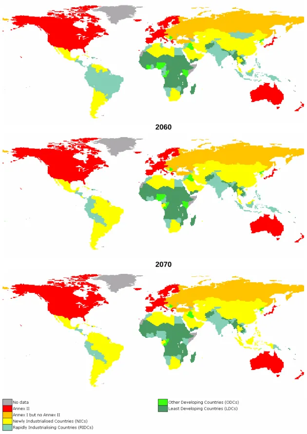
baseline in 2020. Voor het behalen van de stringente doelstellingen zal een grote groep van landen behorende tot deze landen, maar ook de rest van de ontwikkelingslanden in 2020, al in 2030-2040 de status krijgen van de nieuwe geïndustrialiseerde landen.

(8)

(9)

Summary

This report documents a quantitative analysis of the emission and cost implications of the South–North Dialogue Proposal for the differentiation of countries’ future mitigation commitments. This is a proposal outlining equitable approaches to mitigation – including deep cuts in emissions of both the Annex I and Annex II countries, and differentiated mitigation commitments for developing countries. These are divided into four country groups on the basis of an index composed of indicators for responsibility, capability and potential to mitigate. These are: 1) the newly industrialised countries (NICs), 2) the rapidly developing countries (RIDCs), which would have to take on quantitative mitigation

commitments, 3) the other developing countries (Other DCs) and 4) the least developing countries (LDCs), which only have qualitative mitigation commitments (policies and measures).

The tool used for the analysis of the countries’ emission allowances is the FAIR 2.1 world model, the country version of the FAIR 2.1 model, which uses an improved methodology for the downscaling of the population, GDP and emissions data of the IMAGE 2.2 IPCC SRES baseline scenarios to the level of individual countries. The report analyses a “political willingness” scenario and four other scenarios leading to stabilisation of greenhouse gas concentrations at 400, 450, 500 and 550 ppm CO2-equivalent. The

stabilisation scenarios show what the emission reductions are required to reach greenhouse gas concentration in the long-term, and simply assume that Parties will be politically willing to make the necessary effort, whereas the “political willingness” scenario starts from what Parties might be willing to do − or at least one set of assumptions about what “political willingness” might look like. The “political willingness” scenario requires reductions of about 20% below 1990 levels for the Annex I countries in 2020, i.e. the EU-25 (-30%) and the USA (-15%). Under this scenario, stabilisation of CO2-equivalent

concentrations at 500 ppm is kept within reach up to 2020, but substantial reductions have to occur thereafter. It seems unlikely that this scenario will limit global average temperature change to 2 oCelsius. Even more ambitious reduction targets for the Annex I countries will be necessary under the 400 and 450 ppm CO2-equivalent scenarios, which provide more

certainty about limiting global average temperature change to 2 oCelsius, i.e. 30% to 35% below 1990 levels in 2020, and about 80 to 90% in 2050. The NIC emission allowances could grow up to 2010, but then would need to be reduced substantially. RIDCs are assumed to reduce emissions slightly below baseline emissions, but to reach the low emission levels in 2050, a large group of countries in the RIDC group, but also Other DCs and LDCs in 2020, would have to move to the NIC country group as early as around 2030-2040.

(10)

(11)

1 Introduction

The proposal, “South–North Dialogue – Equity in the Greenhouse” (hereafter referred to as the South–North Dialogue Proposal), was designed by researchers from13 industrialised and developing countries. It offers guidance on the content of a future climate agreement and the process of achieving it (Ott et al., 2004). The proposal outlines equitable

approaches to mitigation, including both deep cuts in the emissions of the North and differentiated mitigation commitments for developing countries. It further examines adaptation, as no agreement will be equitable or adequate if it fails to incorporate appropriate funding and institutional mechanisms to address the needs of the most vulnerable to the impacts of climate change. Finally, the proposal includes

recommendations on the political process of achieving such an agreement by outlining a leadership strategy. The proposal is described in detail in Ott et al. (2004) and Winkler et al. (2005) http://www.south-north-dialogue.net.

This report focuses only on the part of the proposal dealing with mitigation commitments, and tries to assess the implications of the proposal for costs and emission allowances1 when combined with different long-term greenhouse gas concentration stabilisation levels. This should help both the drafters of the proposal and others to evaluate the appropriateness of the proposal in arriving at an equitable approach for differentiating mitigation

commitments. But first of all, let us look at a more detailed description of how the mitigation commitments are defined in the proposal.

Mitigation commitments for the South–North Dialogue Proposal

The focus of the ultimate objective of the United Nations Framework Convention on Climate Change (UNFCCC) in Article 2, namely “to achieve stabilisation of greenhouse gas concentrations in the atmosphere” under specified constraints, indicates a consensus among Parties to take action on mitigation. The problem the world is facing is not whether mitigation is important, but rather “who” is mitigating and “how much” is being mitigated. According to the UNFCCC the developed countries should take the lead in mitigation. This is reflected in the Kyoto Protocol, where only the industrialised countries (Annex I) have (quantified) mitigation commitments. The fact that the developed countries need to take the lead implies that at some stage developing countries will be expected to follow. What is required in thinking beyond 2012, therefore, is further and more systematic differentiation among countries, also in the South.

Article 3.1 of the UNFCCC states that such a differentiation should be in accordance with Parties “common but differentiated responsibilities and respective capabilities” (…)

(UNFCCC, 1992). The South–North dialogue proposal thus proposes that the differentiation should be based on the criteria of responsibility, capability and potential to mitigate. These three characteristics are integrated into a differentiation framework as follows:

• Responsibility refers to the Parties’ responsibility for the problem. This was defined

in an earlier attempt by the “Brazilian Proposal” directly in relation to Parties’ overall contribution to temperature increase (UNFCCC, 1997). In the South–North Dialogue proposal, by contrast, cumulative per capita emissions of fossil CO2 over the 1990 to

2000 period are used as a proxy indicator of responsibility. The relatively recent period avoids ‘punishing’ countries for historical emissions, since the consequences

1_{In the literature also referred to as assigned amounts, emission permits, or emission endowments; from this}

(12)

were less widely known in the past. Since the IPCC’s First Assessment Report in 1990, the implications can, at least, be said to be well-known internationally. 2

• Capability refers here to the country’s ability to pay for and implement mitigation

efforts; this criterion recognises the fact that a country’s capability to reduce emissions might be quite different from its level of responsibility. A country may have great responsibility for contributing GHG emissions, but be too poor to devote resources toward mitigation and/or it might not have access to the necessary

technologies. Emissions do not have to be linked to human development, but under given socio-economic and technological conditions, a certain level of emissions will be necessary to guarantee a decent life for poor people (Pan, 2002). Two indicators of capability are considered: the Human Development Index (HDI) and Gross Domestic Product (GDP) per capita. Countries with higher levels of national income and a higher rank on the HDI are expected to carry a higher burden of mitigation.

• Potential (to mitigate) refers to a country’s opportunities for reducing GHG

emissions and can be related to two factors – intensity of the emissions and emissions per capita. A high value for CO2/GDP would suggest a high potential to mitigate. The

more efficient an economy already is (lower CO2 emissions per unit GDP), the less

potential there is (at a given cost) to mitigate further through efficiency. However, the level of emissions per capita needs to be taken into account as well. High per capita emissions suggest unsustainable consumption patterns, which should provide

potential to mitigate without endangering a basic level of development, for example, through lifestyle changes. National circumstances such as resource endowments also influence mitigation potential.

Based on these criteria of responsibility, capability and potential, the South–North dialogue proposal concludes that the first level of differentiation in the Convention – i.e. between Annex I and non-Annex I, remains valid. As a consequence, it is obvious that Annex I countries must continue to take the lead in reducing emissions, and their emissions reductions should be strengthened considerably in the period after 2012.

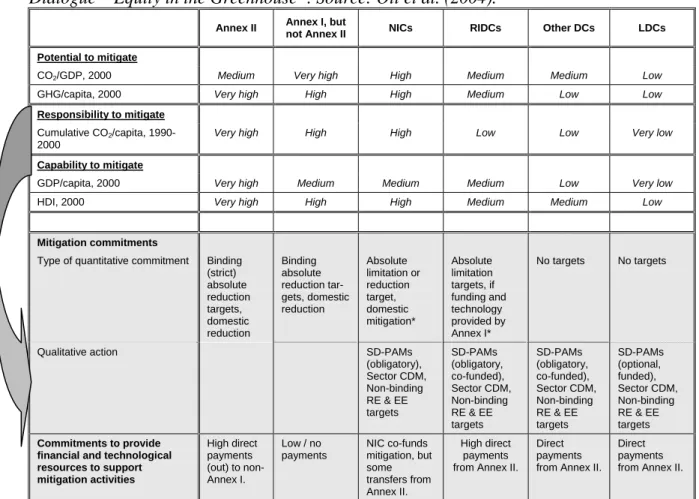
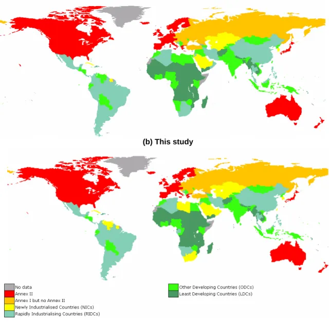
The Proposal defines four groups of non-Annex I countries, each including countries with similar national circumstances. The first two are the newly industrialised countries (NICs) and the rapidly industrialising developing countries (RIDCs). Both groups are considered particularly important in taking the next round of climate negotiations forward. The two other groups are the least-developed countries (LDCs), and “other developing countries” the latter consisting of countries not belonging to any of the previous groups. The last two groups are both excluded from taking on quantitative commitments (Table 1). This

grouping of the non-Annex I countries is based on an index combining the criteria of responsibility, capability and potential to mitigate. This index is defined by the equal

weighting of cumulative fossil CO2 emissions per capita, the Human Development Index

and an indicator of potential (derived from CO2 emissions/GDP and greenhouse gas

emissions/capita).

(13)

Table 1. Regions and their responsibility according to the proposal “South–North Dialogue – Equity in the Greenhouse”. Source: Ott et al. (2004).

Annex II Annex I, but

not Annex II NICs RIDCs Other DCs LDCs Potential to mitigate

CO2/GDP, 2000 Medium Very high High Medium Medium Low

GHG/capita, 2000 Very high High High Medium Low Low

Responsibility to mitigate

Cumulative CO2/capita,

1990-2000

Very high High High Low Low Very low

Capability to mitigate

GDP/capita, 2000 Very high Medium Medium Medium Low Very low HDI, 2000 Very high High High Medium Medium Low

Mitigation commitments

Type of quantitative commitment Binding (strict) absolute reduction targets, domestic reduction Binding absolute reduction tar-gets, domestic reduction Absolute limitation or reduction target, domestic mitigation* Absolute limitation targets, if funding and technology provided by Annex I* No targets No targets

Qualitative action SD-PAMs (obligatory), Sector CDM, Non-binding RE & EE targets SD-PAMs (obligatory, co-funded), Sector CDM, Non-binding RE & EE targets SD-PAMs (obligatory, co-funded), Sector CDM, Non-binding RE & EE targets SD-PAMs (optional, funded), Sector CDM, Non-binding RE & EE targets Commitments to provide financial and technological resources to support mitigation activities High direct payments (out) to non-Annex I. Low / no payments NIC co-funds mitigation, but some transfers from Annex II. High direct payments from Annex II.

Direct payments from Annex II.

* Targets only could become binding if all major Annex I countries have binding quantified emission reduction obligations.

It should be noted that LDCs, which by definition have low potential, low capability and low responsibility, form a distinct analytical group. The remaining non-LDC non-Annex I countries are then ranked by this index. NICs are identified as those countries with an index value more than one standard deviation above the mean, i.e. those with the highest

aggregate score. The next group of non-Annex I countries with a medium index value (mean plus/minus one standard deviation) are defined as RIDCs. RIDCs are generally characterised by having experienced relatively rapid industrial growth in the last decade and a relatively high income. RIDCs are therefore selected more from the remaining non-Annex I countries, i.e. those with higher per capita GDP-PPP than the non-non-Annex I average per capita GDP-PPP and a higher than 2% annual GDP growth in 1991-2000. Finally, the remaining 39 non-Annex I countries that are neither NICs/RIDCs nor LDCs are grouped as “other developing countries”. These are at a very early stage of industrialisation but are not as poor as those countries defined as “least developed” or just – in short: “regular”

developing countries.

Based on the three criteria applied for the differentiation of countries (responsibility, capability and potential to mitigate), a set of decision rules was developed. This resulted in the following types of commitments for the six country groups identified (see Table 1, two groups in Annex I, four in non-Annex I):

• Both Annex I groups – Annex II and others – retain Kyoto-style quantitative

commitments, i.e. (binding) quantified (absolute) emissions reduction obligations with targets for Annex II countries being more demanding than Kyoto levels. The latter will

(14)

also be committed to financial and technological transfers to those non-Annex I countries with low-to-medium capability to mitigate.

• Countries belonging to the group of NICs and RIDCs will have to take on quantitative mitigation commitments as well – although subject to the conditionality that all major Annex I countries (including the USA) take on quantified emission reduction

commitments and fulfil their commitments to provide financial and technological resources. Due to their high responsibility and potential to mitigate, NIC countries will have absolute limitation or reduction commitments, but will also have access to

financial and technological resources (from Annex II countries) to help them fulfil the commitments. RIDC countries would also take on absolute limitation targets, and would have access to an even greater share of resources than the NICs, consistent with their lower capacities. However, the conditionality concerning Annex I participation in the regime is also valid for RIDCs, as well as the availability of full funding of

incremental costs for mitigation activities by Annex II countries. Regardless of whether the terms of conditionality for quantified commitments are fulfilled, NICs and RIDCs will engage in qualitative mitigation commitments, such as sustainable development policies and measures (Winkler et al., 2002), sectoral CDM (Samaniego and Figueres, 2002; Sterk and Wittneben, 2005) or voluntary renewable energy or energy efficiency targets (see Table 1).

• Qualitative mitigation commitments (policies and measures) will also be obligatory for the group of “other developing countries”, but quantifiable mitigation commitments for these countries and the LDC group are not justifiable – and not in line with the decision rules (until their status changes).

There must be agreed conditions (like “binding obligations for all major industrialised countries”) that will lead to the start of developing-country quantitative emission targets. While these conditions can be quantitatively defined, even more important is getting political agreement on what they should be. They further differ from graduation triggers in that they may include conditions for both developing and industrialised countries.

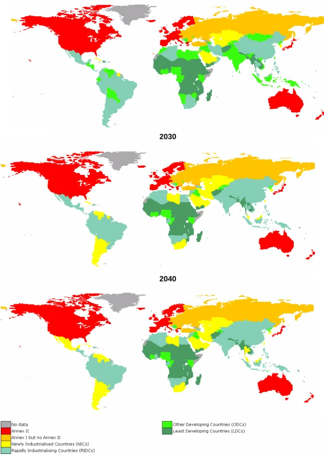
The approach chosen for differentiation of the (types of) commitments among countries is not static. As national circumstances in countries evolve over time, the composition of the groups will change. If a country exceeds (or falls below) a certain threshold (valid for all of the three criteria – potential, responsibility, capability to mitigate) it will move from one group to another and, as a consequence, will have to take on other types of commitments. Countries “graduate” when their indicators become more representative of the following higher group. Therefore, the composition of the groups may need to be modified after each commitment period.

Differences with an earlier analysis of the proposal

This report uses the methodology of Höhne and Ullrich (2005)3 for calculating the emission allowances under the South–North Dialogue Proposal, including a method on how to decide which countries belong to which country group over time. This is supplemented with a methodology for calculating the abatement costs and financial flows resulting from emission trading. Only financial flows associated with quantified emissions commitments in the South-North Dialogue Proposal are evaluated. The methodology does not quantify the effect of qualitative commitments, e.g. SD-PAMs (obligatory), sectoral CDM and non-binding targets of the proposal, as this requires more detailed, disaggregated, sectoral energy modelling. For the quantification of the financial funding related to the support of

3_{The methodology here is almost the same, except that in Höhne and Ullrich the definition of RIDCs is}

without the additional condition on economic growth and income level, which in their analysis leads to a larger group of RIDCs.

(15)

(the incremental costs of) mitigation activities in NICs, RIDCs, simple assumptions have been made. The methodology also includes the financial flows resulting from the use of the Kyoto Mechanisms (particularly international emissions trading).

The study of Höhne and Ullrich was the first quantitative analysis of the emission allowances under this Proposal. Note that Höhne & Ullrich and this study use the same definition of the emission allowances, i.e. CO2-equivalent emissions including the

anthropogenic emissions of six Kyoto greenhouse gases (fossil CO2, CH4, N2O, HFCs,

PFCs and SF6 (using the 100-year GWPs IPCC, 2001)), but excluding LUCF (land-use and

land-use change-related) CO2 emissions.4 The analysis presented here differs in five ways

from the analysis of Höhne and Ullrich:

1. Baseline scenarios at the level of individual countries are based on an improved

(non-linear) downscaling method that tries to deal with the limits of present downscaling methods. Both studies make use of the IMAGE implementation of the IPCC SRES

emission scenarios (hereafter simply referred to as: IMAGE IPCC SRES scenarios) at the level of 17 world regions5, but Höhne and Ullrich (2005) use a different

methodology for downscaling the regional information of population, GDP and emissions to the level of countries (about 192). Höhne and Ullrich used the regional trend to downscale the information, i.e. applied the regional growth rates for all countries belonging to a region (hereafter also referred to as the linear down-scaling method). This linear downscaling method was also used by Gaffin et al. (2004) for downscaling the population (for 2050–2100)6 and GDP (2000-2100) data of the original IPCC SRES emission scenarios defined at the level of the four IPCC regions. However, this linear downscaling method has been criticised in the literature (see Pitcher, 2004; van Vuuren et al., 2005), as it leads to unrealistic results.7 In particular, it falls short in cases where the differences in historical trends and absolute levels between countries in a region are too large. This happens, for example, in the region of East-Asia, including China, North Korea, South Korea, Mongolia and Taiwan, where it can lead to

extremely high income levels for countries considerably richer than their neighbouring countries (e.g. especially South Korea compared to the population-dominant region of China).

The linear downscaling method of Höhne and Ullrich (2005) results in similar problems. On the one hand, the problems are likely to be even more severe than for Gaffin at al., as the method is now applied to a longer time horizon (population projections up to 2050 and emissions up to 2100), while, on the other, they may be less, as they used information at the level of 17 regions instead of the four IPCC regions. This is illustrated in Text box 1 and Appendix A, and in more detail in van Vuuren et al. (2005).8

4_{Emissions from these sources are highly uncertain and emission estimates from various sources are often not}

consistent. Therefore it has also been suggested to treat emissions from deforestation with an instrument separate from other emissions (WBGU, 2003).

5_{Canada, USA, OECD-Europe, Eastern Europe, FSU, Oceania and Japan (Annex I regions); Central}

America, South America, Northern Africa, Western Africa, Eastern Africa, Southern Africa, Middle East & Turkey; South Asia (incl. India), East Asia (incl. China), South-East Asia (non-Annex I regions) (IMAGE-team, 2001).

6_{For the 2000-2050 period Gaffin et al. (2004) used an existing scenario on a country level and the relative}

positions of countries within the larger unit as the basis for the downscaling. This method was not criticised in Pitcher’s review.

7_{Pitcher (2004) concluded that the shortcomings of using the regional trend in Gaffin et al. (2004) were so}

severe that most of the results do not provide a satisfactory basis for doing research.

8_{The country level baseline scenarios of Höhne and Ullrich were also used for the post-2012 regime analyses,}

as described in Höhne et al. (2004; 2005). An earlier study of Höhne et al. (2003) used this downscaling method for the IPCC SRES emission scenarios (Nakicenovic et al., 2000) at the level of the four IPCC SRES regions, where it fails even more, given the larger differences between countries in each region.

(16)

Text box 1. The impact of the linear downscaling method vs. the non-linear downscaling methods on projections of a country’s baseline population, per capita income and emissions Table 2 gives the downscaled information of countries’ population, per capita income and

emissions in 2050 of the IMAGE 2.2 IPCC SRES scenarios of the linear downscaling method used by Höhne and Ullrich (2005), and of the non-linear downscaling method of van Vuuren et al. (2005) used by this study. The absolute numbers here represent the median over the six IMAGE 2.2 IPCC SRES scenarios. It also presents the relative differences, i.e. comparing the relative growth factors compared to the 2000 levels for both studies, which only reflect the differences due to the downscaling method, and not due to differences in the 2000 estimates. These relative differences correspond with the numbers in the last column in Table A.1, A.2 and A.3 in Appendix A. The table depicts the first ten countries, with a population of at least 10 million persons, with the highest differences. This is followed by the first five countries, with again the highest differences, for a population of at least 100 million persons. It also gives the global estimates. The last row gives the average of all relative differenced (in absolute terms) for all countries.

The table shows that the average (relative) difference for population projections in 2050 will be as high as about 25%, with a difference of more than 50% for some African and Asian countries, and also for Cuba, South Africa (almost 90%) and Afghanistan (almost 52%). For per capita income, the highest difference (as mentioned before) for some Asian countries is more than 100%, such as Singapore (about 130%) and South Korea (about 120%), with per capita income levels far

exceeding the Annex I per capita income levels. The average difference over all the countries is now even almost 27%. For the emissions, we find very high differences for some Asian and African countries. Table 2 also shows that aggregates of the linear-downscaling method used by Höhne and Ullrich (2005) may differ from the global estimate of the original IMAGE 2.2 IPCC scenarios (for example, global 2050 per capita income is about 15% higher), whereas the methodology of van Vuuren et al. (2005) is always consistent with the original source, by ensuring that aggregation retains the original dataset. Finally, the data for both studies at the level of all countries are compared in Appendix A.

Table 2. The countries’ population, per capita income and emissions in 2050 of the IMAGE 2.2 IPCC SRES scenarios of the linear downscaling method used by Höhne and Ullrich (2005) v, and of the non-linear downscaling method of van Vuuren et al. (2005) used in this study, and its relative difference. The absolute numbers here represent the median over the six scenarios.

Population (millions) – 2050 Per capita income (1000PPP$/capita) Emissions (in MtCO2) – 2050

Country

Linear downscaling Non

-lin

ear

downscaling Relative differen

ce

* (%)

-lin

ear

ce

*

-lin

ear

ce

*

1 Kenya 68.1 35.2 92.7 Singapore 128.9 53.8 130.1 Burundi 34.4 12.1 337.0 2 South Africa 96.2 51.5 89.6 Korea (South) 10.6 41.3 120.9 Uganda 523.4 87.1 203.7 3 Zimbabwe 28.0 16.4 71.6 Korea (South) 91.2 48.9 109.3 Kenya 420.4 313.3 173.4 4 Cuba 16.3 9.7 67.9 Taiwan 121.2 102.0 94.9 Senegal 152.2 80.9 131.6 5 Yemen 38.2 94.0 -60.2 United Arab. E 93.1 83.4 94.4 Ethiopia 466.3 231.8 129.4 6 Cameroon 33.0 21.2 58.0 Cyprus 85.4 37.0 93.8 Ghana 151.0 96.8 114.6 7 Angola 29.2 62.4 -55.9 Qatar 124.7 87.5 92.5 Congo 15.9 24.7 91.1 8 Afghanistan 33.6 68.5 -51.7 Gabon 39.9 19.9 85.1 Mali 54.7 80.1 77.5 9 Niger 24.0 49.0 -51.4 Slovenia 86.2 44.2 83.4 Namibia 26.0 27.1 71.4 10 Sri Lanka 29.3 19.1 50.1 Israel 87.3 47.3 76.3 Eritrea 197.4 14.2 67.2

Countries with more than 100 million persons

Turkey 138.6 99.8 42.2 Russian Fed. 52.7 32.3 42.0 Dem. Rep. Congo 241 175 59.3 Pakistan 218.4 332.0 -33.6 India 19.5 15.6 24.6 India 8670 7549 18.2 Iran 146.2 107.7 28.2 Iran 23.1 30.1 -16.7 Russian Fed. 3348 3805 -17.3 Dem. Rep. Congo 113.1 135.8 -20.6 Congo 5.9 5.1 16.5 Mexico 1426 1704 -14.6 Russian Federation 150.8 133.5 13.0 Mexico 41.6 35.7 16.1 Nigeria 1275 857 13.4

Global 8583 8629 -1.3 Global 22.1 22.5 -3.5 Global 71782 80174 10.0

Average difference 25.5 Average difference 27.3 Average difference 26.2

v _{The baseline scenarios on a country level from Höhne and Ullrich were also used for the post-2012 regime analyses, as described in}

(17)

Text box 1. Continued

Concluding, the linear downscaling method used by Höhne and Ullrich (2005) does not provide a satisfactory set of results, and leads to completely different results from the non-linear downscaling method by van Vuuren et al. (2005) used here. It should be noted that as emission allowances calculated are dependent on the baseline scenarios used, these are also highly affected by the use of the downscaling methods. In fact, as illustrated above and in Appendix A, the impact of the

downscaling methods may be of more importance than the assumed reductions under a post-2012 regime for differentiation of future commitments for quite a few countries (in particular, the developing countries). This report will not analyse the impact of the downscaling methods used in the emission allowances in much detail as this is not the main focus of this study.

This study uses a set of downscaling algorithms based on recent work of van Vuuren (2005). The recently published long-range population projections on a country level by the UN (UN, 2004b) are used for downscaling population data. For downscaling GDP and emissions, van Vuuren et al. assumed a convergence of countries’ per capita income and emissions per GDP to the average regional level. A form of convergence is likely to occur within larger regions – and has also been assumed in the IPCC SRES storylines. In this way, these downscaling algorithms try to deal with the shortcomings of the earlier methods using a regional trend, and thereby provide much more plausible results for population, GDP and emissions projections.

2. Historical and base-year greenhouse gas emissions are based on the same data as in

the original study, namely the CAIT 2.0 database of the World Resource Institute

(WRI) (http://cait.wri.org), whereas Höhne and Ullrich (2005) make use of national emission inventories submitted to the UNFCCC and, where not available, existing emission databases.

3. More consistent calculations of the multi-gas emission pathways and emission

allowances. Höhne and Ullrich (2005) make use of CO2-only emission pathways

stabilising the CO2 concentration at 400 and 450 ppm CO2-only (Höhne et al., 2005).

For the calculating the countries’ emission allowances, they use the global CO2-only

emission targets (relative to 1990 levels) for the global CO2-equivalent emission targets

(including the six Kyoto greenhouse gases, but excluding LUCF CO2) by assuming the

same trend for the non-CO2 greenhouse gases as for CO2. This assumption does not

seem realistic given the time-dependent share of non-CO2 gases in the reductions in

multi-gas strategies using Global Warming Potentials (GWPs). In other words, the contribution of the non-CO2 gases in total reductions is very large early in the scenario

period, but the focus in the long-term is still CO2 (van Vuuren et al., 2003). However,

assuming the same trend for the fossil CO2 emissions and land-use related (LUCF) CO2

emissions seems unlikely, as the present baseline (non-intervention) scenarios already shows strong decreases in the LUCF CO2 emissions compared to the present levels

(IMAGE-team, 2001).

This study uses the recently developed set of multi-gas emission pathways for different CO2-equivalent concentration9 stabilisation levels, i.e. 400, 450, 500 and 550 ppm

CO2-equivalent (den Elzen and Meinshausen, 2005a; 2005b), compatible with levels of

certainty for adequately keeping the global mean surface temperature increase below 2o Celsius above pre-industrial levels (see section 2). The calculations of the countries’ emission allowances make use of the global CO2-equivalent emission targets of the

emission pathways, which are both calculated in terms of CO2-equivalent emissions of

9_“CO

2 equivalent concentration” summarises the climate effect (“radiative forcing”) of all human-induced

greenhouse gases, tropospheric ozone and aerosols, following the IPCC definition, as if we only changed the atmospheric concentrations of CO2 (see Schimel et al., 1997).

(18)

the six Kyoto greenhouse gases (excluding LUCF CO2). This methodology seems more

consistent, as it better accounts for the time-dependent share of non-CO2, LUCF CO2

and fossil CO2 emissions in the global CO2-equivalent emission pathways.

4. Multi-gas emission pathways allow for an overshoot in the concentration levels, and the

result is less stringent short-term Annex I and Annex II reduction commitments. For the

400, 450 and 500 ppm CO2-equivalent concentration targets, this study assumes a

certain overshooting (or peaking); i.e. concentrations are allowed to peak before

stabilising (going up to 480-500 ppm CO2-equivalent before going down to levels such

as 400 or 450 ppm CO2-equivalent later on). This overshooting is partially reasoned by

the already substantial present concentration levels and the attempt to avoid drastic sudden reductions in the emission pathways presented (den Elzen and Meinshausen, 2005a; 2005b). The CO2-only emission pathways of Höhne and Ullrich (2005) do not

allow for such an overshoot in concentrations, which leads to high, and maybe “unrealistic” fast and deep emission reduction commitment, in particular for the 400 ppm CO2-only scenario, for the Annex I countries in the short-term (2020-2025).10

Such deep reductions seem politically, technically and economically unfeasible. The short-term global CO2-equivalent emission targets are less stringent in this study

(section 3). For example, the global emissions target for 2020 for the most stringent concentration target (400 ppm CO2-equivalent) correspond with Höhne and Ullrich’s

450 ppm CO2-only target (about 500-525 ppm CO2-equivalent). An overall result of the

study are the less stringent short-term reduction commitments for all countries, in particular, the Annex I countries.

5. Abatement costs and financial flows. Besides the emission allowances, as presented in the two studies, this report also outlines the abatement costs and financial flows at the level of individual countries.

Build-up of the report

Section 2 starts by providing the set of multi-gas emission pathways, while section 3 describes the tool, the FAIR 2.1 world model, used for the analysis of the emission allowances. This model is essentially a country version of the FAIR 2.1 model, the policy-decision support tool for analysing emission allowances and abatement costs at the level of world regions. The FAIR 2.1 world model makes use of the baseline scenarios at the level of individual countries. Section 4 describes the assumptions made to quantify the emissions allowances under the South–North Dialogue Proposal. The next two sections present the countries’ emission allowances for the “political willingness scenario” (Section 5) and for the four scenarios leading to stabilisation of CO2-equivalent concentration at 400, 450, 500

and 550 ppm, respectively (Section 6). The stabilisation scenarios show what the emission reductions are required to reach greenhouse gas concentration in the long-term, and simply assume that Parties will be politically willing to make the necessary effort, whereas the “political willingness” scenario starts from what Parties might be willing to do − or at least one set of assumptions about what “political willingness” might look like. Section 6 also presents abatement costs and financial flows for the four scenarios. Section 7 summarises the conclusions.

10_{Höhne and Ullrich concluded: “The 400 ppm scenario requires yet more ambitious reduction by all}

countries, which are at the limit of what some would call realistic. Annex II countries would need to cut emissions in half by 2020 and RIDCs and NICs would follow quickly.”

(19)

2 Multi-gas emission pathways to stabilise long-term

greenhouse gas concentrations

This section presents a set of multi-gas emission pathways for different CO2-equivalent

concentration stabilisation levels, i.e. 400, 450, 500 and 550 ppm CO2-equivalent, along

with an analysis of implied probability of adequately keeping global mean surface temperature increase below 2°C above pre-industrial levels. This work is based on the study of den Elzen and Meinshausen (2005a; 2005b). The applied methodology focuses on a cost-effective division among different greenhouse gas reductions for given emission limitations on GWP-weighted and aggregated emissions. Thus, the model framework reflects the existing policy framework with present caps on GWP-weighted overall

emissions under the assumption of cost-minimising national strategies. The emissions that are iteratively adapted to meet the pre-defined stabilisation targets include those of all the major greenhouse gases (fossil CO2, CH4, N2O, HFCs, PFCs and SF6), ozone precursors

(VOC, CO and NOx) and sulphur aerosols (SO2).

Den Elzen and Meinshausen (2005a) have developed the emission pathways for three baseline scenarios, the IMAGE IPCC B1 scenario (a low-level emissions scenario) and the Common POLES IMAGE (CPI) baseline (a medium-level emissions scenario) (van Vuuren et al., 2003; 2004b) scenario. This was done with both default Marginal Abatement Costs (MAC) curves, and the CPI+tech scenario, with baseline emissions based on the CPI scenario and fixed LUCF CO2 emissions of the IMA-B1 scenario (less deforestation) and

MAC curves assuming additional technological improvements. Here, we focus on the emission pathways under the CPI+tech scenario, as this is a medium-level emissions scenario, leading to feasible emission pathways for the (low) 400 and 450 ppm CO2

-equivalent concentration targets, whereas for the CPI scenario there were no feasible pathways for these concentration levels.

The emission pathways presented aim at stabilisation of the long-term greenhouse gas concentrations at CO2-equivalence levels of 550, 500, 450 and 400 ppm. As already

mention in section 1, a “peaking strategy” is followed here: i.e. concentrations may first increase to an “overshooting” concentration level up to 480, 500 and 525 ppm then decrease before stabilising at 400, 450 and 500 ppm CO2-equivalence, respectively. This

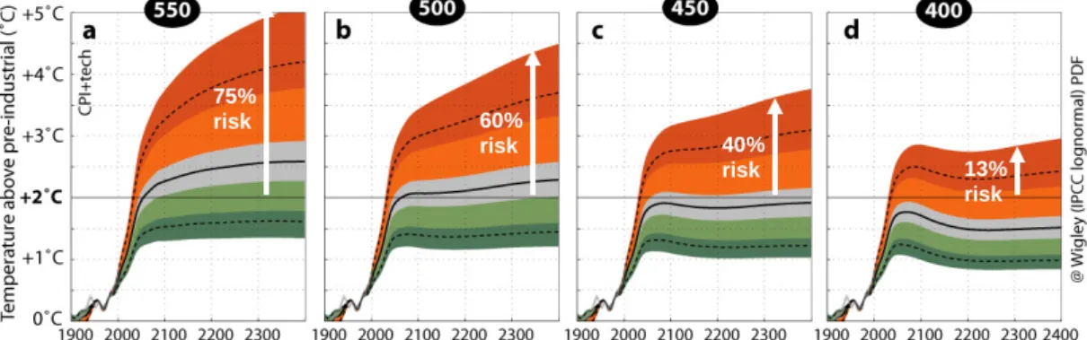
peaking is partially reasoned by the already substantial present net forcing levels (Hare and Meinshausen, 2004) and the attempt to avoid drastic sudden reductions in the emission pathways presented. shows the probabilistic temperature implications (for 2000-2400) of the emission pathways based on the climate sensitivity Probabilistic Density Function (PDF) of Wigley and Raper (2001).11 The natural forcings (i.e. solar and volcanic forcings) are included in these transient calculations of den Elzen and Meinshausen (2005a), (see for more details, Hare and Meinshausen (2004).12

Figure 1 shows that an emission pathway leading to 550 ppm CO2-equivalent stabilisation

is unlikely to adequately limit global mean temperature increase below 2°C above pre-industrial level (Figure 1). In order to adequately limit global temperature increase below 2°C with a probability of more than 60% (85%) (assuming the probabilistic density function of Wigley and Raper, 2001), greenhouse gas concentrations need to be stabilised to below 450 (400) ppm CO2-equivalent or lower. If a different climate sensitivity PDF is

11_{The PDF of Wigley and Raper (2001) assumes the conventional 1.5 to 4.5°C climate sensitivity uncertainty}

range as being a 90% confidence interval of a lognormal PDF.

12_{An exception has been made for the calculations on the risk of overshooting the 2°C limit in equilibrium.}

There, equilibrium temperatures have been directly derived from anthropogenic radiative forcings (Hare and Meinshausen, 2004). See, for example, Figure 1 - the number on the white arrows.

(20)

assumed, for example, the one by Murphy et al. (2004), the probability still sharply increases with lower stabilisation levels, although the risk of overshooting generally

increases. Specifically, stabilisation at 450 (400) ppm CO2-eq. would imply a probability of

achieving 2°C of about 22% (66%).

The emissions of the pathways for stabilisation at 550, 500, 450 and 400 ppm CO2-eq.

concentrations (for the 1990-2060) can be summarised in their GWP-weighted sum of emissions of six Kyoto gases, as illustrated in Figure 2. Clearly, there are different pathways that can lead to the ultimate stabilisation level. Den Elzen and Meinshausen (2005a) have assumed that the global emission reduction rates should not exceed an annual reduction of 2.5%/year for all default pathways (at least not over longer time periods). The reason is that a faster reduction might be difficult to achieve given the inertia in the energy production system: electrical power plants, for instance, have a technical lifetime of 30 years or more. Fast reduction rates would require early replacement of existing fossil-fuel-based capital stock, which may be associated with large costs. A maximum rate of 2%/year is hardly ever exceeded for the majority of the post-SRES mitigation scenarios, apart from some lower stabilisation scenarios. As a result of this (the assumed onset of reductions from the baseline emissions), reduction takes place relatively early, and global emissions peak around 2015-2020. For all stabilisation pathways, the global reduction rates remain below 2.5%/year for the whole scenario period, except for the pathways at 400 ppm CO2-eq., with maximum reduction rates of 2.5-3%/year over 20 years.13

Figure 1. The probabilistic temperature implications for the stabilisation pathways between

1900 and 2400 at (a) 550 ppm, (b) 500 ppm, (c) 450 ppm and (d) 400 ppm CO2-equivalent

concentrations for the CPI+tech baseline scenario based on the climate sensitivity PDF by Wigley and Raper (2001) (IPCC lognormal). The median (solid lines) and 90% confidence interval boundaries (dashed lines) are shown, as well as the 1%, 10%, 33%, 66%, 90%, and 99% percentiles (borders of shaded areas). The historical temperature record and its uncertainty from 1900 to 2001 is shown by the grey shaded band (Folland et al., 2001). Source: den Elzen and Meinshausen (2005a).

By 2050, global greenhouse gas emissions (excl. LUCF CO2), basically the Kyoto gas

emissions, will have to be near 40-45% below 1990 levels for stabilisation at 400 ppm CO2-eq. For higher stabilisation levels, e.g. 450 ppm CO2-eq., greenhouse gas emissions

(excl. LUCF CO2) may be higher, namely 15-25% below 1990 levels. The reduction

requirements become as high as 50 to 55% (30 to 40%) below 1990 levels for stabilisation

13_{A further delay in the peaking of global emissions in 10 years doubles maximum reduction rates to about}

5% per year, and will very likely lead to high costs (den Elzen and Meinshausen, 2005a).

75% risk 13% risk 40% risk 60% risk

(21)

at 400 ppm CO2-eq (450 ppm CO2-eq) in 2050 for all greenhouse gas emissions, including

LUCF CO2.

For the analysis of this report, eight reference points of global greenhouse gas emission levels excluding LUCF CO2 emissions in 2020 and 2050 were selected; these have to be

met by all approaches for the following quantification of emission allowances. These are based on the rounded-off percentages (to the nearest multiple of 5%) from the CPI+tech scenario, as the emissions of this scenario are in the middle of the emissions for the six IPCC SRES scenarios, which are used in the calculations in this study.

2020 2050 400ppm 20 -45 450ppm 30 -25 500ppm 35 -5 550ppm 40 10 +35% +40% +20% - 5% +10% -45% -25% +30% 2020 2050 400ppm 20 -45 450ppm 30 -25 500ppm 35 -5 550ppm 40 10 2020 2050 400ppm 20 -45 450ppm 30 -25 500ppm 35 -5 550ppm 40 10 +35% +40% +40% +20% +20% - 5% +10% -45% -25% - 5% - 5% +10% +10% -45% -45% -25% -25% +30% 2020 2050 400ppm 20 -45 450ppm 30 -25 500ppm 35 -5 550ppm 40 10

Figure 2. Global emissions relative to 1990, excluding LUCF CO2 emissions between 1990

and 2060, for the stabilisation pathways at 550, 500, 450 and 400 ppm CO2-equivalent

concentrations for the CPI+tech scenario. The global reduction targets used (dots) for the analysis of emission allowances of the South–North Dialogue Proposal are also given here.

(22)

(23)

3 The FAIR 2.1 world model: a tool to analyse

countries’ emission allowances and abatement costs

The tool used for the analysis of the emission allowances and abatement costs, the FAIR 2.1 world model, is briefly described here. But first we will briefly review the FAIR 2.0 model, the foundation of the FAIR 2.1 world model.

3.1 The FAIR 2.0 model

The policy decision-support tool, FAIR 2.0 (Framework to Assess International Regimes for the differentiation of commitments) (den Elzen and Lucas, 2003; 2005b) was developed to explore and evaluate the environmental and abatement cost implications of various

international regimes for differentiation of future commitments for meeting such long-term climate targets as stabilisation of the atmospheric GHG concentrations. There have been many proposals for differentiating commitments among countries, both from literature and from Parties to the UNFCCC (see Aldy et al., 2003 for an overview; Bodansky, 2004; Kameyama, 2004; Torvanger and Godal, 2004). The FAIR 2.0 model includes about ten approaches, all defining the differentiation of commitments based on criteria and rules for the distribution of emission allowances (i.e. allocation-based approaches, see also section 2). The model does not comprise approaches for differentiating commitments in terms of outcomes, such as equal mitigation costs (Babiker and Eckhaus, 2002), as these are dependent on a macro-economic model (not included in the FAIR model). “Policies and Measures” approaches, such as technology and performance standards including energy-efficiency standards (e.g. Barrett, 2001; Edmonds and Wise, 1999), financial measures (e.g. Schelling, 2002) and carbon taxes (Cooper, 2001) (for an overview, see Bodansky, 2004; den Elzen and Berk, 2004) have not been implemented, as this requires more detailed, aggregated, sectoral energy modelling. The model focuses on multi-lateral regimes based on the UNFCCC and the Kyoto Protocol, and not on regimes based on smaller coalitions between like-minded parties, the most important players or collaboration at the regional level. This approach is often combined with a pledge-based approach with countries’ commitments based on their “willingness to pay”. While the model allows for simulating such an approach, its focus is on evaluation of rule-based approaches to defining

international commitments.

The FAIR 2.0 model can be used for a consistent and quantitative comparison of various allocation-based, multi-lateral regime proposals, as has been done, for example, for the EU DG Environment project, “Greenhouse gas reduction pathways in the UNFCC post-Kyoto process up to 2025” (Criqui et al., 2003; den Elzen et al., 2003; van Vuuren et al., 2003). The model was also used to evaluate the Kyoto Protocol under the Bonn and Marrakesh agreements in terms of environmental effectiveness and costs (den Elzen and de Moor, 2001; 2002a; 2002b; Lucas et al., 2005), the Bush Climate Change Initiative (van Vuuren et al., 2002) and the Brazilian Proposal (den Elzen et al., 2003; 2005b; den Elzen and

Schaeffer, 2002; 2005d). Furthermore, the model was used to support dialogues between scientists, NGOs and policy makers (e.g. Berk et al., 2001). To this end the model is set up as an interactive tool with a graphical interface, allowing for interactive changing and viewing model input and output.14 Other scientific applications of the FAIR 2.0 model are, in combination with the integrated assessment model IMAGE15 and the energy model

14_{A demonstration version of FAIR 2.0 can be downloaded from:}_{http://www.mnp.nl/fair}_.

15_{The IMAGE 2.2 model is an integrated assessment model, consisting of a set of integrated models that}

(24)

TIMER16, the analysis of multi-gas mitigation scenarios in the Emission Modelling Forum (EMF 21) (van Vuuren et al., 2004b).

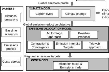
Historical emissions Baseline scenarios Costs curves Emissions profiles DATSETS Regional GHG emissions after trade

Abatement costs & permit price Mitigation costs &

Emissions trade COST MODEL

Climate change CLIMATE MODEL

Global emission profile

Regional emissions targets Contraction & Convergence Multi-Stage approach Emission Intensity Targets EMISSIONS ALLOCATION MODEL

Brazilian Proposal Triptych approach Global climate indicators Carbon cycle

Global emission reduction objective

Figure 3. Schematic diagram of the FAIR model showing its framework and linkages (den Elzen and Lucas, 2003; 2005b).

The FAIR model consists of three linked models (Figure 3): 1. A climate model to calculate the climate impacts of global emission profiles and emission scenarios, and to determine the global emission reduction objective – based on the difference between the global emissions scenario (without climate policy) and a global emission profile (den Elzen and Schaeffer, 2002; den Elzen et al., 2002; 2005d); 2. An emission allocation model to calculate the regional emission allowances for different regimes for the differentiation of future commitments within the context of this global reduction objective (from climate model) (den Elzen, 2002; den Elzen and Berk, 2003; den Elzen et al., 2005a; den Elzen et al., 2003; 2005c); 3. A costs model to calculate the emission targets after emissions trading and regional abatement costs on the basis of the emission allowances (from the emission allocation model) follows a least-cost approach, making full use of the flexible Kyoto mechanisms like emissions trading and substitution of reductions between the different gases and sources (den Elzen and de Moor, 2002a; den Elzen et al., 2005c; Lucas et al., 2005). Furthermore, various data sets of historical emissions, baseline scenarios, multi-gas emission pathways and costs curves are included in the model framework to assess the sensitivity of the outcomes towards these key inputs. Calculations were done for 17 regions, i.e. Canada, USA, OECD-Europe, Eastern Europe, FSU, Oceania and Japan (Annex I regions); Central America, South America, the Middle East and Turkey (middle- and high-income non-Annex I regions); Northern Africa, Southern Africa, East Asia (incl. China) and South-East Asia (low-middle income non-Annex I regions) and Western Africa, Eastern Africa and South Asia (incl. India) (low-income non-Annex I regions) (IMAGE-team, 2001).

agriculture and energy use, atmospheric emissions of greenhouse gases and air pollutants, climate change, land-use change and environmental impacts (IMAGE-team, 2001).

16_{The global energy model, TIMER 1.0 (as part IMAGE), describes the primary and secondary demand and}

production of energy and the related emissions of greenhouse gasses and regional air pollutants (de Vries et al., 2002).

(25)

3.2 The FAIR 2.1 world model

A logical next step after the realisation of the FAIR 2.0 model (2003) was to extend the calculations of the emission allowances and abatement costs to the level of countries, as individual countries are the actors in the international negotiations and countries’ emission profiles may be very different even within one geographic region, e.g. South Korea and China. Hence, individual countries are interested in the implications of various approaches for their emission levels.

However, to date (2005) good reliable data of baseline emission scenarios at the level of all world countries have not been available. The existing downscaling methods to downscale the information on population, GDP and emissions of the IPCC SRES scenarios the level of regions to the level of countries, were strongly criticised in literature (see Pitcher, 2004; van Vuuren et al., 2005), as leading to unrealistic results (in particular the one using the regional trend, as used by Gaffin et al., 2004; Höhne et al., 2003; Höhne et al., 2005). A recently developed new downscaling method by van Vuuren et al. (2005) has changed this situation. This method is used for downscaling the information of the same indicators of the IMAGE IPCC SRES scenarios of the IMAGE-team (2001) at the level of the 17 IMAGE world regions to countries and deals with the limits of the existing downscaling methods. For downscaling the population data, the long-range population projections on a country level recently published by the UN (2004b) are used. For downscaling GDP and emissions, van Vuuren et al. assumed a convergence of countries’ per capita income (in US$ or PPP$) and emissions per GDP to the average regional number. This downscaling method assumes (partial) convergence of the units to the average regional number, making sure that the total of the elements complies with the pathway of the larger unit. For several parameters, there are good reasons to assume that some form of convergence within larger global regions is likely to occur – certainly in some of the SRES storylines. This is a very logical assumption in the case of large differences between units in a region result in unlikely outcomes in cases of linear downscaling. It is also a very logical assumption if (partial) convergence also occurs between regions. The rate of convergence can be influenced by choosing a convergence year. A detailed description of the methodology can be found in van Vuuren et al. (2005).

The FAIR 2.1 world model (still under development) makes use of this downscaled

information of the IMAGE IPCC SRES scenarios at the level of the 192 UN countries (e.g., den Elzen and Lucas, 2005a). This FAIR 2.1 world model can be used for doing quantitative analyses of emission allowances and abatement costs for post-2012 climate regimes for commitments at the level of individual countries, using a set of baseline scenarios at the level of countries, as has been done in this study.17

The basis of the FAIR 2.1 world model is formed by the FAIR 2.1 model (under

development), which is an update of the FAIR 2.0 model with its calculations still at the level of 17 world regions (completely in line with the IMAGE IPCC SRES scenarios); this

includes updated multi-gas emission pathways (see section 2 and den Elzen and

Meinshausen, 2005a; 2005b); historical data using as base year 2000 (instead of 1995) (see this report), updated climate attribution calculations (den Elzen et al., 2005b; den Elzen et al., 2005d); an updated Triptych approach (based on the work of Phylipsen et al., 2005), and

17_{Höhne et al. (2003) were the first to present countries’ emission allowances for post-2012 climate regimes,}

but they used a set of baseline scenarios for population, GDP and emissions at the level of countries, based on applying the regional downscaling method for the IPCC SRES emission scenarios (Nakicenovic et al., 2000) from the four IPCC SRES regions to 192 countries, that was criticised in the literature as being unrealistic. In their follow-up studies (Höhne et al., 2005; Höhne and Ullrich, 2005) they applied the growth rates of the IPCC SRES implementation of the 17 IMAGE regions at the level of countries.

(26)

two additional post-2012 regimes for post-2012 commitments (i.e.

Common-but-differentiated convergence (Höhne et al., 2004) and the South–North Dialogue Proposal (this report). See also den Elzen and Lucas (2005a) and improved costs calculations with the most recent EMF costs curves (den Elzen and Meinshausen, 2005a; den Elzen et al., 2005c; van Vuuren et al., 2004b).

The FAIR 2.1 world model is essentially the same as the FAIR 2.1 model, but now the calculations of emission allowances at the level of 192 UN countries and of abatement costs at the level of 51 countries and/or groups of aggregated countries instead of the 17 regions (see Appendix B). The main specific components of the FAIR 2.1 world model, which differ from the FAIR 2.1 region model, are described below:

• Historical data – The base-year (2000) population data is provided by the UN World Population Prospects (UN, 2004a). The national per capita income levels in the base-year (in US$ or PPP$)18 are based on the 2004 database World Development Indicators (WorldBank, 2004). For the missing countries in this database, the set is supplemented with the series “GDP, at constant 1990 prices – US dollars” from the UN Statistics Database (2005), using a conversion from 1990 to 1995 prices. The historical (1990-2000) countries’ GHG emissions are based on the CAIT 2.0 database

(http://cait.wri.org). More specifically, the CO2 emissions from fossil fuel combustion

and cement production (1765-2000) are based on the CDIAC database (Marland et al., 2003) and IEA data (IEA, 2002).The CO2 emissions from land-use changes

(1950-2000) are based on Houghton (2003). The non-CO2 Kyoto GHG emissions (CH4, N2O

the HCFCs, HFCs, PFCs and SF6) (1990-2000) are based on the EPA (2004) and

EDGAR 3.2 (Olivier and Berdowski, 2001), and where data for 2000 data were

missing, these were estimated by WRI. For alternative calculations, the FAIR 2.1 world model also includes the national inventories submitted to the UNFCCC for the base-year emissions and, where these inventories are not available, other sources (based on the same databases as mentioned above) are used. This database is the same as the one used by Höhne et al. (2005).

• Countries’ baseline scenarios – Baseline scenarios are used for future (2000-2100) projections of the countries’ population and GDP (in US$ or PPP$), along with the anthropogenic baseline emissions of the Kyoto greenhouse gases. The different baseline scenarios included are the six IMAGE implementation of the six IPCC SRES scenarios (IMAGE-team, 2001; Nakicenovic et al., 2000) and the Common POLES-IMAGE baseline emission scenario (van Vuuren et al., 2003; van Vuuren et al., 2004b). These scenarios all occur at the level of the 17 IMAGE world regions. Here, a set of

algorithms is used for the downscaling of this information from the 17 world regions to the 192 countries (van Vuuren et al., 2005), as described earlier in this section.

• 2012 emission targets – Up to 2012, implementation of the Annex I Kyoto Protocol targets is assumed for all Annex I countries (for the EU countries these are the internal EU burden-sharing targets) excluding Australia and the USA.19 Although the USA aims at the proposed greenhouse-gas intensity target (White-House, 2002), this does not lead

18_{The Purchase Power Parity (PPP) is an alternative indicator for GDP per capita, based on relative}

purchasing power of individuals in various regions, i.e. the value of a dollar in any country, or, in other words, the dollars needed to buy a set of goods compared to the dollars needed to buy the same set of goods in the USA.

19 _{Although included in the model, the default calculations here do not analyse the impact of other}

implementations of the Kyoto Protocol: i.e. (1) a “strong” Kyoto implementation, in which the USA and Australia also implement their Kyoto targets and the emissions of economies in transition (Russia and Eastern European countries) follow the lower of their Kyoto targets and their baseline emissions, and their ‘hot air’ will not be sold. Neither do the default calculations analyse (2) a “failure” of the Kyoto Protocol, in which all countries implement their baseline emissions, since implementation of both, the “strong” Kyoto

(27)

to emissions that are significantly different from their baseline emissions (van Vuuren et al., 2002). Note that the economies in transition (Russia and Eastern European countries) follow their Kyoto targets, leading to some excess emission allowances in 2012, and these Kyoto targets will also be used as the starting point for calculating their post-2012 emission allowances.20 The non-Annex I regions follow their assumed baseline emissions up to 2012.

The calculations of the abatement costs are valid for 51 countries (including groups of aggregated countries, as listed in Appendix B), and make use of the baseline emission scenarios for 192 countries and the Marginal Abatement Cost (MAC) curves21 for 17 regions for CO2 and 19 regions or countries for non-CO2 greenhouse gases.

• Marginal Abatement Cost (MAC) curves are used for the 17 regions, six Kyoto

greenhouse gases and different numbers of sources (for example, for CO2 (12), CH4(9),

N2O (7). Technological developments, learning effects and system inertia are

schematically taken into account by using time-dependent MAC curves (described in den Elzen and Lucas, 2005b; van Vuuren et al., 2004a; 2004b). For more details about the costs calculations we refer to Section 6.2.

20_{The assumptions on the targets for the USA and economies in transition are different from those assumed in}

Höhne and Ullrich (2005), in which a “strong” Kyoto implementation was assumed (see previous footnote).

21_{MAC curves reflect the costs of abating the last ton of CO}

2-equivalent emissions and, in this way, describe

(28)