a) Corresponding author. E-mail: a.tiktak@rivm.nl
RIVM report 500026001/2005
Modelling the interactions between transient saturated and unsaturated groundwater flow
Off-line coupling of LGM and SWAP
F.J. Stoppelenburg, K. Kovar, M.J.H. Pastoors and A. Tiktaka
This investigation has been performed by order and for the account of the Directorate-General of the RIVM within the framework of project M/500026, ‘Soil and Groundwater Models’.
Het rapport in het kort
Modellering van de interactie tussen de waterstroming in de bodem en het grondwater. Koppeling van LGM en SWAP.
Het Landelijk Grondwatermodel (LGM) en een één-dimensionaal model van de hydrologie van de onverzadigde zone (SWAP) zijn gekoppeld. Met dit gecombineerde model kunnen de waterstromen in het bodem- en grondwatersysteem, alsmede de stromingen vanuit het grondwater naar het oppervlaktewater, berekend worden. Het model kan zodoende de hydro-logische invoer leveren voor studies naar de belasting van grond- en oppervlaktewater met nutriënten en gewasbeschermingsmiddelen. Een andere mogelijke toepassing van het model is de simulatie van de variatie van de grondwaterstand in de tijd. Om de seizoensdynamiek correct te kunnen berekenen, worden zowel LGM als SWAP dynamisch toegepast. Het model kan op verschillende schalen worden toegepast. De prestaties van het model zijn getoetst in een studie in het Beerze Reusel gebied. In het algemeen bleek dat de overeenkomst tussen de gemiddelde diepte van het grondwaterpeil, zoals berekend met SWAP, goed overeenkwam met de gemiddelde diepte van het grondwaterpeil, zoals berekend met LGM. Ook bleek dat beide modellen de seizoensdynamiek op dezelfde wijze simuleren. Een aanvullende studie moet aantonen in hoeverre de berekende grondwaterpeilen overeenkomen met de gemeten grondwaterpeilen. Deze studie moet aangeven of het gecombineerde model de hydrologische basis kan leveren voor verdrogingstudies en waterkwaliteitsberekeningen, zoals die door het Milieu- en Natuurplanbureau worden uitgevoerd.
Abstract
Modelling the interactions between transient saturated and unsaturated groundwater flow. Off-line coupling of LGM and SWAP
The groundwater flow model for the Netherlands (LGM), and a one-dimensional model of soil water flow (SWAP) were coupled. With this combined model, it is possible to calculate fluxes and residence times of nutrients and pesticides in both the unsaturated zone and the phreatic aquifer. The model can also predict the seasonal dynamics of the groundwater table. In order to correctly simulate these seasonal dynamics, both LGM and SWAP are used in transient mode. The performance of the model was tested in a regional-scale model applica-tion. There was generally a good agreement between the mean depth of the groundwater ta-ble, as simulated with SWAP, and the mean depth of the groundwater depth as simulated by LGM. The seasonal dynamics of the groundwater table were, however, underestimated by LGM. Further investigation showed that correct transfer of the phreatic storage coefficient was the key factor for correctly predicting the seasonal dynamics of the groundwater table. With the correct storage coefficient, the correspondence between the groundwater heads simulated by SWAP and the groundwater heads simulated by LGM were nearly perfect. An additional study should show whether there is also a good agreement with observed ground-water heads. Results from this study can be used to conclude upon the applicability of the adopted methodology for both ecohydrological studies and water quality assessments as re-quired by the Netherlands Environmental Assessment Agency.
Key words: hydrology; groundwater; surface-water; LGM, SWAP; modelling; coupling;
Contents
Samenvatting... 9 Summary ... 11 1. Introduction ... 13 1.1 General introduction 13 1.2 Overview of report 13 1.3 Perspectives 14 2. Model description... 152.1 Theory of the Groundwater Model for the Netherlands (LGM) 15
2.2 Theory of SWAP 18
2.3 The coupling concept 19
3. Derivation of the spatial schematisation and model parameterisation... 29
3.1 Spatial schematisation 29
3.2 Parameterisation of LGM 30
3.3 Parameterisation of SWAP 36
4. Performance of the coupled model at the regional scale... 39
4.1 Introduction 39
4.2 Description of study region Beerze-Reusel 39
4.3 Model set-up 40
4.4 Convergence between SWAP and LGM 42
4.5 Performance of the coupling procedure 43
4.6 Discussion and conclusions 48
5. Application on a national scale... 51
5.1 Two-step modelling approach 52
5.2 Results 54
5.3 Summary and conclusions 60
6. Conclusions and recommendations... 63 References ... 65 Appendix 1 Improved method for coupling of LGM and SWAP... 67
Samenvatting
Dit rapport beschrijft de koppeling tussen het Landelijk Grondwatermodel (LGM) en een één-dimensionaal model van de hydrologie van de onverzadigde zone, SWAP. Met dit ge-combineerde model kunnen de waterstromen in het bodem- en grondwatersysteem, alsmede de stromingen vanuit het grondwater naar het oppervlaktewater, berekend worden. Het model kan zodoende de hydrologische invoer leveren voor studies naar de belasting van grond- en oppervlaktewater met nutriënten en gewasbeschermingsmiddelen. Een andere mogelijke toe-passing van het model is de voorspelling van de variatie van de grondwaterstand in de tijd, bijvoorbeeld gedurende het jaar. Informatie over deze jaarlijkse fluctuaties is met name van belang in studies naar de effecten van verdroging op ecosystemen, waar de diepte van de grondwaterstand in het begin van het groeiseizoen gebruikt wordt als een indicator voor de vochttoestand. Om de seizoensdynamiek correct te kunnen berekenen, worden zowel LGM als SWAP dynamisch toegepast; de uitwisseling van gegevens tussen beide modellen vindt per decade plaats. Aangezien verdrogingstudies in het algemeen een groot ruimtelijk detail vereisen, zijn procedures geïmplementeerd om de resultaten van het gecombineerde model met een hoge ruimtelijke resolutie beschikbaar te maken. De ruimtelijke schematisatie van het model is daarom flexibel gemaakt; de basisgegevens worden hierbij via GIS procedures rechtstreeks naar effectieve modelparameters vertaald. De prestaties van het model zijn ge-toetst in een studie in het Beerze Reusel gebied. In het algemeen bleek dat de overeenkomst tussen de gemiddelde diepte van het grondwaterpeil, zoals berekend met SWAP, goed over-eenkwam met de gemiddelde diepte van het grondwaterpeil, zoals berekend met LGM. Het bleek echter ook dat de seizoensdynamiek onderschat werd door LGM. Nadere studie leerde dat dit veroorzaakt werd doordat de zogenaamde freatische bergingscoëfficiënt onjuist van SWAP naar LGM werd overgedragen. Nadat dit hersteld was, was er een nagenoeg perfecte overeenkomst tussen de grondwaterstand berekend door SWAP en de grondwaterstand bere-kend door LGM. Toetsing aan gemeten grondwaterpeilen heeft nog niet plaatsgevonden. Een aanvullende studie, waarin de resultaten van het gecombineerde model met grondwaterstan-den gemeten in het Nederlandse zandgebied worgrondwaterstan-den vergeleken, kan op korte termijn worgrondwaterstan-den uitgevoerd. Deze studie moet aangeven of het gecombineerde model de hydrologische basis kan leveren voor verdrogingstudies en waterkwaliteitsberekeningen, zoals door het Milieu- en Natuurplanbureau worden uitgevoerd.
Summary
An offline coupling was established between the groundwater flow model for the Nether-lands, LGM, and a one-dimensional model of soil water flow, SWAP. With this combined model, it is possible to calculate fluxes and residence times of chemicals (particularly nutri-ents and pesticides) in both the unsaturated zone and the phreatic aquifer. Because the model considers interactions with local surface-water systems, the model can be used to predict fluxes of these chemicals into surface waters as well. Another possible application of the model is the prediction of the seasonal dynamics of the groundwater table, which is particu-larly important in ecohydrological studies, where the depth of the groundwater table at the start of the growing season is an important indicator of water availability. In order to cor-rectly simulate these seasonal dynamics, both LGM and SWAP are run in transient mode, with a coupling time-step of 10 days. Procedures have been implemented to make the final results available at a very high spatial resolution, which is a requirement for ecohydrological studies. Regardless the grid size, GIS procedures convert the basic model parameters avail-able in the LGM database into effective model input parameters. The performance of the combined model was tested in a regional-scale model application. There was generally a good agreement between the mean depth of the groundwater table, as simulated with SWAP, and the mean depth of the groundwater depth as simulated by LGM. The seasonal dynamics of the groundwater table were, however, underestimated by LGM. Further investigation showed that correct transfer of the phreatic storage coefficient was the key factor for correctly predicting the seasonal dynamics of the groundwater table. After adaptation of the calculation of this coefficient, the correspondence between the groundwater heads simulated by SWAP and the groundwater heads simulated by LGM were nearly perfect. The model has not yet been validated against observed groundwater heads; this should be done in an additional study to be carried out soon. Results of this study can be used to conclude upon the applica-bility of the LGM-SWAP model as the hydrological modelling tool for both ecohydrological studies and water quality assessments as required by the Netherlands Environmental Assess-ment Agency.
1.
Introduction
1.1 General introduction
The Groundwater Model for the Netherlands (LGM) is a model for the simulation of quantity and quality aspects of saturated groundwater systems. The model has been developed by the National Institute of Public Health and the Environment, RIVM (Pastoors, 1992; Kovar et al., 1992) and was applied in various studies. The focus in these studies was on effects of groundwater abstractions on the geohydrological system (Leijnse and Pastoors, 1996). Later, studies were carried out to quantify contamination of drinking water abstraction wells with nutrients and pesticides (Kovar et al., 1998; Kovar et al., 2000; Uffink and Van der Linden, 1998; Tiktak et al., 2004). Since the mid nineties, attention in the policy arena shifted from drinking water to ecohydrological studies and to diffuse source pollution of the shallow groundwater and local surface waters by nutrients and pesticides. These problems require an adapted model approach, in which the mutual relationships between the unsaturated zone, the saturated zone and local surface waters are considered. For this reason, RIVM, Alterra and RIZA together developed the hydrological component of the nutrient fate model STONE (Wolf et al., 2003). This model consists of an offline coupling between the unsaturated zone model SWAP (Van Dam, 2000) and the National Groundwater Model (De Lange, 1996). Al-though this model has successfully been used in the evaluation of the Dutch Manure Policy (RIVM, 2004), it suffered from a number of limitations:
− the model showed an unrealistic, long-term trend in the groundwater table for approxi-mately 10% of the cases;
− the model could not reproduce the seasonal dynamics of the groundwater table, which is required for ecohydrological studies;
− the spatial schematisation of the model was fixed. It was therefore not possible to make local refinements, which are needed for ecohydrological studies and regional studies. To mitigate to these problems, RIVM decided to accomplish an offline coupling between the Groundwater Model for the Netherlands (LGM, version 4) and the SWAP model (ver-sion 2.0.9d). The most important additional requirements for this model are:
− the model should be able to correctly describe both the long-term trend and the seasonal dynamics of the groundwater table;
− the model should be operational at different spatial scales, using finite-element grids of any required spatial resolution.
1.2 Overview of report
After this general introduction, an overview of the model and the coupling procedure is given in chapter 2. The spatial schematisation and the model parameterisation is discussed in chap-ter 3. Chapchap-ter 4 and 5 describe some model applications. In chapchap-ter 4, the combined model is applied in a catchment. The aim of this application was to test the performance of the cou-pling procedure. Chapter 5 describes the application of the model at the national scale. An
important aim of this application was to test the ability of the model to operate at different spatial scales, with local grid refinements. Final conclusions and recommendations are re-ported in chapter 6. A user manual of the model is published in a separate report (Tiktak et al., 2004).
1.3 Perspectives
Due to its flexible set-up, the current model can be used at different spatial scales. The fol-lowing model outputs are calculated in a consistent way:
− long-term trends and seasonal dynamics of fluxes of water into the shallow groundwater and local surface waters;
− long-term trends and seasonal dynamics of hydrological state variables, the most impor-tant one being the groundwater table.
The model can provide the hydrological base for desiccation studies and ecohydrological studies. The model can also provide inputs for such studies as the evaluation of the ‘Dutch Manure Policy’ and the evaluation of the ‘Policy Plan Sustainable Crop Protection’.
2.
Model description
2.1 Theory of the Groundwater Model for the Netherlands (LGM)
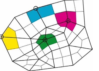
The Groundwater Model for the Netherlands (LGM version 4) is a model for the simulation of quantity and quality aspects of saturated groundwater systems. LGM was developed by the National Institute of Public Health and the Environment, RIVM (Pastoors, 1992; Kovar et al., 1992) and applied in various studies (for example, Leijnse and Pastoors, 1996; Kovar et al., 1998; Kovar et al., 2000).LGM simulates groundwater flow in a saturated multi-aquifer geohydrogical system consist-ing of a series of aquifers separated by aquitards. The flow in the system is assumed to be quasi three-dimensional, namely two-dimensional horizontal flow in aquifers and vertical flow in aquitards. LGM is based on the numerical technique of finite elements. The elements are quadrilaterals and triangles. The model can be applied for any user-selected grid density, the grid density being dependent on the specific conditions of the problem to be solved. The grid can be locally refined, for example within a well capture area or in the vicinity of rivers. Figure 2.1 shows schematically the basic features of the LGMs finite element implementa-tion, namely the grid nodes, the elements, and the node influence areas, Ainf (m2).
Figure 2.1. Example of a finite element grid for LGM, containing nodes, elements and node influence areas Ainf (dashed lines). Influence areas are highlighted at four nodes.
The basic module of LGM calculates groundwater heads in aquifers, the flux across the aqui-tards, the flux between the top aquifer and rivers, and the flux between the top aquifer and the small-scale surface water system (ditches, drains, brooks). The latter flux is referred to as the topsystem flux.
In the current study, LGM was applied in transient mode, with two time-variable inputs, the groundwater recharge rate, qre (m d-1), and the storage coefficient of the top aquifer, µ (-). All
abstrac-tion rates, river water levels, and drainage levels in the small-scale surface water systems, were kept constant in time.
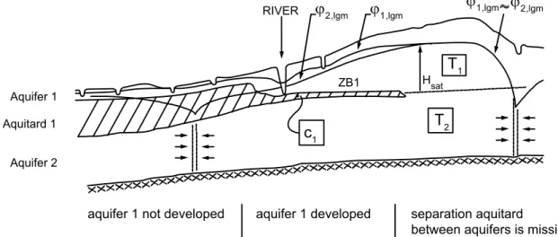
Figure 2.2 depicts the geohydrological system in the Groundwater Model for the Netherlands. Although usually five aquifers are used for national studies, for simplicity the figure is re-stricted to two aquifers. LGM calculates, as a function of time, the groundwater heads in the first and second aquifers, respectively. An essential part of the schematisation is that the up-permost aquifer (aquifer 1) is phreatic. The latter means that the upup-permost aquifer is not overlain by a semi-pervious layer. This implies that the upper boundary of the uppermost aquifer is at the ground surface. Depending on the occurrence and depth of the first aquitard, three situations can be distinguished:
– regions where no aquifer occurs immediately below ground level, such as in peat-clay polder areas shown in the left part of figure 2.2. In these cases, a very thin dummy top aquifer will be modelled with negligible horizontal flow. This horizontal flow does not make part of any (sub)regional flow. It is markedly local in nature, being shallow ground-water flow to the nearest ditches. Obviously, groundground-water abstractions are not permitted in this dummy top aquifer;
– regions where both the top aquifer and the separating aquitard exist, as shown in the cen-tral part of figure 2.2. The modelled top aquifer stretches between the aquitard top and the ground surface;
– regions where only one thick aquifer exists from the base up to the ground level, but the separating aquitard is missing. This is shown in the rightmost part of figure 2.2. In this case a dummy aquitard (with small hydraulic resistance c1) has to be introduced, thus
split-ting the actual aquifer into the top aquifer and aquifer 2. In those regions LGM will calcu-late the groundwater head φ1,lgm ≈ φ2,lgm. It is possible that the calculated groundwater head
φ1,lgm can be below the bottom level of the top aquifer, as is shown in figure 2.2.
RIVER c1 T2 T1
.
ϕ2,lgm Hsat ϕ1,lgm ϕ1,lgm ϕ2,lgm Aquifer 1 Aquitard 1 Aquifer 2 ZB1aquifer 1 not developed aquifer 1 developed separation aquitard
between aquifers is missing Figure 2.2. Sketch of the geohydrological system of the Groundwater Model for the Netherlands. c1 is
the hydraulic resistance of the separating aquitard and T1 and T2 are the transmissivities of the
Unlike the transmissivity T2 (m2 d-1), which is a user-given input value, the transmissivity
T1 (m2 d-1) of the top aquifer (aquifer 1) depends on the current value of the calculated
groundwater head φ1,lgm. T1 follows from the equation:
(
1,lg 1)
1 kHsat k m ZT
T = = ϕ − (2.1)
where k (m d-1) is the horizontal hydraulic conductivity within the top aquifer, H
sat (m) is the
saturated thickness of the top aquifer, and ZT1 is the height of the bottom of the uppermost
aquifer. The value of the saturated thickness Hsat is minimised to 0.1 m to ensure that T1
re-mains a small positive value, which on its turn implies negligible horizontal flow in the top aquifer.
In LGM, two types of surface waters are distinguished, namely rivers and small surface wa-ters. Small surface waters are represented by a lumped ‘top-system relationship’ and are dif-fuse in nature. On the other hand, in the finite element grid of LGM, rivers follow their actual location in space.
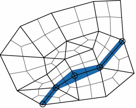
Figure 2.3. Rivers in LGM, coinciding with element sides. Dashed lines delineate the node influence areas (see also figure 2.1).
The rivers represent large (wide) river courses, like the Rhine and its major branches. They also include large canals, like the ‘Amsterdam Rijn Channel’. Figure 2.3 illustrates the loca-tion of a river, the river being located along the element sides between five nodes. All river-related parameters can be variable along the water course. Those parameters are the river width, the hydraulic resistance of the river bottom, and the river-water level. In each river node, the flux between the top aquifer and the river, Qriv is defined by:
(
riv m)
rivriv
riv A h c
where Qriv (m3 d-1) is the flux from the river to the groundwater in the top aquifer, Ariv (m2) is
the surface area of the river within the influence area of a node, hriv (m) is the water level of
the river, and criv (d) is the hydraulic resistance of the river bottom. As mentioned before,
though LGM allows the river-water level hriv to be specified variable in time, in this study we
have used a time invariant water level.
The topsystem flux relation regards the interactions between the top aquifer and the small-scale surface waters (ditches, drains, brooks). The topsystem flux qts (m d-1) is assumed to be
constant within an influence area of a node, the total topsystem flux Qts [m3 d-1] at a node
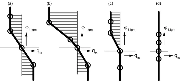
be-ing expressed by Qts = Ainf qts. Figure 2.4 illustrates the shape of the topsystem relation for
LGM. The relation is composed of a series of topsystem points, each topsystem point being defined by a groundwater head hts and a flux qts occurring at hts. Values of qts smaller than
zero and qts larger than zero indicate a drainage and infiltration situation, respectively. The
multiple piecewise relations in figure 2.3 are created by concatenating a series of separate flux-head relationships existing in a given node, for example the relation for the primary sys-tem (see page 21 for definitions of drainage syssys-tems), the relation for the secondary syssys-tem, and the relation for the surface drainage. Note that the number of points in the topsystem rela-tion for LGM is identical at all grid nodes. Consequently, if no relarela-tion exists in a node or the relation is less complex than in other nodes, dummy topsystem points are introduced to pre-serve the same number of topsystem points for all nodes.
(a) (b) (c) (d) ϕ1,lgm ϕ1,lgm ϕ1,lgm ϕ1,lgm qts qts qts qts
Figure 2.4. Examples of shape of the topsystem flux relation in LGM, each with four topsystem points: (a) one drainage/infiltration system with one dummy point on top, (b) one drainage/infiltration system combined with one drainage system, (c) one drainage system with two dummy points, and (d) absence of any infiltration and drainage system (four dummy points, each with qts=0).
2.2 Theory of SWAP
The Soil Water Atmosphere Plant (SWAP version 2.0.9d) model is a one-dimensional, dy-namic, multi-layer model. An extensive overview of the SWAP model is given by Van Dam et al. (1997) and Van Dam (2000).
The SWAP model (Van Dam, 2000) uses a finite-difference method to solve Richard’s equa-tion. The hydraulic properties are described by closed form functions as proposed by Van Genuchten (1980). The upper boundary of the model interacts with the atmosphere, and is situated at the top of the crop canopy (figure 2.5). Daily rainfall fluxes are input to the model; the reference evapotranspiration rate is calculated from daily temperature and radiation data, according to Makkink (1957). The lower boundary of the system is used to interact with the regional groundwater system and was located at a depth of 13 m below soil surface. In this study, a Cauchy type of boundary condition was chosen, which is further described in sec-tion 2.3). The lateral boundary of the system consist of local surface water systems that inter-act with the groundwater. In SWAP, a maximum of five different classes of local drainage systems can be considered. All drainage systems are spatial distributed and have a linear rela-tionship between drainage flux and groundwater level.
precipitation transpiration evaporation of intercepted water soil evaporation throughfall fluctuating groundwater level soil water fluxes ponding water uptake by plant roots seepage lateral discharge to ditches and field-drains uns atur at ed z one sa turated z one crop calendar surface run-off
Figure 2.5. Overview of processes included by SWAP, as such considered in the coupled LGM-SWAP model (after Tiktak et al., 2003).
2.3 The coupling concept
2.3.1 Basic principles
In the Netherlands, the groundwater level is generally shallow and the drainage system dense. As a result, there is a strong interaction between the regional groundwater system, the local drainage system and the unsaturated zone. The feedback between the unsaturated zone and the saturated zone is particularly strong in the case of shallow groundwater tables. The maximum depth of the groundwater table, where interdependence plays a role, depends pri-marily on the soil physical properties. For example, the depth reach of interdependence for a
coarse-sandy soil is significantly smaller than that for a loamy fine-sandy soil. A numerical experiment investigating the importance of the feedback mechanism is presented by Stoppe-lenburg et al. (2002).
An important point in the current coupling concept is that both SWAP and LGM simulate the interaction with local drainage systems (the topsystem flux). For this reason, there is a verti-cal overlap between the two models (figure 2.6). This feature of incorporating local drainage fluxes into the SWAP models allows the calculation of residence times of pesticides and nu-trients in the uppermost saturated zone.
SWAP drainage base hydrological basis qre,swa φ2,lgm φ1,lgm aquifer 1 aquifer 2 aquifer 3 qbot LGM c1 cbot
Figure 2.6. Schematic representation of geohydrological system of LGM and SWAP.
Because of the required vertical overlap, the actual link between SWAP and LGM is not car-ried out at the depth of the groundwater table, but at the depth of the uppermost aquitard (fig-ure 2.6). The two variables that are used for the interaction are the vertical flux and the phreatic storage coefficient. The vertical flux is the bottom boundary condition for SWAP and the upper boundary condition for LGM (section 2.3.2). Because of the higher temporal dynamics in the unsaturated zone, SWAP uses a smaller internal time-step than LGM. For this reason, variables obtained from SWAP are averaged in time before being transferred to LGM (section 2.3.3). In order to get a consistent water balance of the phreatic aquifer in both models, the models should be adjusted in an iterative procedure (section 2.3.4). This iteration procedure must account for the interaction with the local drainage systems, as these systems are part of the (overlapping) phreatic aquifer (section 2.3.5).
2.3.2 Exchange of boundary conditions
Bottom boundary condition of SWAP provided by LGM
Frequently used bottom boundary conditions for unsaturated flow models, that are combined with models for regional groundwater flow, are the Neuman flux condition and the head-dependent Cauchy condition. A Neuman flux as the bottom boundary condition has no real linkage with changing phreatic groundwater heads. In case of an online coupling mechanism (1:1 in time) between a saturated groundwater model and an unsaturated flow model this will not lead to major deviations, as the time-step is small enough to provide for the necessary mutual influence. On the other hand in case of an off-line coupling mechanism, especially when a groundwater model calculates with larger time-steps than the unsaturated flow model, there is no sufficient feedback mechanism to adjust the bottom flux to the phreatic groundwa-ter head and vice visa. This can lead to an under- or overestimation of the infiltration-/seepage flux. As a result a systematic decline or rise of the groundwater table can occur, dur-ing the larger simulation time-step of the groundwater model.
As a Cauchy condition for the bottom boundary of SWAP clearly has a mechanism to adjust the bottom flux to the phreatic groundwater head, it has been selected as most appropriate for the LGM-SWAP coupling. The use of the Cauchy condition provides SWAP with a self-adaptive flux that corresponds with the calculation time-step of the SWAP model itself. The boundary condition at the bottom of the soil column of SWAP, qbot (m d-1) is expressed by
(see also figure 2.7):
lgm , left bot bot bot q c q =ϕ2,lgm−ϕ + (2.3)
where ϕ2,lgm (m) is the groundwater head of the second aquifer of LGM, ϕbot (m) is the
groundwater head of the bottom numerical layer of the soil column of SWAP, cbot (d) is the
vertical resistance of the confining layer and qleft,lgm (m d-1) is the left-over flux of the phreatic
aquifer in LGM, which is explained further on.
Notice that not the phreatic head but the groundwater head of the bottom numerical soil layer is used to define the (regional) bottom flux. In order to produce the same flux across the first aquitard in both models the groundwater head difference should be determined considering the same vertical resistance. Taking the groundwater head at the bottom of the soil column instead of the phreatic head, additional vertical resistance caused by a vertical saturated con-ductivity in each of the soil compartments will be excluded this way. This is consistent with LGM. The resistance in the groundwater model fully occurs at the flow across the first aqui-tard (equivalent to the confining layer in SWAP), and no resistance whatsoever takes place for vertical flow in the phreatic aquifer.
At the same time the phreatic head in LGM ϕ1,lgm corresponds in most cases with the phreatic
head in SWAP ϕ1,swa , on condition that in SWAP the reciprocal of the total vertical saturated
φbot = groundwater head at bottom numerical layer (m)
φ2,lgm = groundwater head of 2nd aquifer of LGM (m)
cbot = resistance of confining layer (day) qbot = Cauchy bottom boundary flux (m day-1)
gwl = groundwater table (m)
zi & zi-1= z-levels of bottom soil compartments (m)
bot bot lgm 2, bot
c
q
=
ϕ
−
ϕ
Cauchy :·
g wl·
·
·
·
·
·
·
φ2,lgm φbot zi-1 zi qbot cbot gwlFigure 2.7. Cauchy bottom boundary condition of SWAP.
The leftover flux qleft,lgm (m d-1) is introduced specifically for the coupled LGM-SWAP
model. The leftover flux contains a composed flux of hydrological processes within the phreatic aquifer that are considered by the groundwater model LGM, but are not taken into account by the unsaturated flow Modelling with SWAP. The leftover flux qleft,lgm is
trans-formed from a volume flux (m3 d-1) to a spatial distributed flux (m d-1) and can consist of the following three fluxes:
inf inf inf lg , A Q A Q A Q
qleft m= riv + well + hor (2.4)
where Qriv (m3 d-1) is the volume flux of surface waters incorporated as line-elements in
LGM, Qwell (m3 d-1) is the extraction volume rate of wells in the phreatic aquifer of LGM,
Qhor (m3 d-1) is the net horizontal volume flux of a finite element nod to or from its
neigh-bouring nods, and Ainf (m2) is the influence area of a finite element node in LGM.
Important to mention here is that the left-over flux has to be taken into account only in the vicinity of wells and large surface waters, that are incorporated as line-elements. Further away from these hydrological features the left-over flux has very small values.
Upper boundary condition of LGM provided by SWAP
The transient groundwater model LGM requires values of the groundwater recharge and the phreatic storage coefficient for its top boundary condition. The groundwater recharge qre,swa
(m d-1) is derived from SWAP and is defined as the vertical soil water flow across the groundwater table. A facility is made to assure a smooth transition of the successive daily output values of the groundwater recharge, in case the groundwater table crosses the bound-ary between two soil compartments during a decade (10 days), the calculation time-step of LGM. The groundwater recharge is actually composed of the vertical fluxes above and below the groundwater table. The proportion between the two vertical soil-water fluxes is deter-mined by their distance toward the groundwater table. The groundwater recharge qre,swa
(m d-1) is expressed as follows: − − + − − = − − − − i i i 1 i 1 i 1 i z z z gwl qv z z gwl z qv q i i swa re 1 , (2.5)
where qvi-1 and qvi (m d-1) are the vertical soil water fluxes above and below the groundwater
table respectively, zi-1 and zi (m) are the bottom boundaries of the soil compartments i-1 and i,
and gwl (m) is the groundwater level, all negative downwards.
The phreatic storage coefficient µ (m3 m-3) is determined over the entire unsaturated column and is given by:
∑
∑
= = − = gwl gwl n i i n i i i act sat D D 1 1 ) (θ θ µ (2.6)where θsat (m3 m-3) is the volumic saturated soil water content, θact (m3 m-3) is the actual
volumic soil water content, Di (m) is the thickness of the soil compartment i and ngwl the
number of soil compartments above the groundwater table.
In cases of deep groundwater tables there is a chance that the entire soil column of SWAP becomes unsaturated. In these situations it is not possible to make use of the Cauchy condi-tion as the bottom boundary condicondi-tion. Therefore, in cases of deep groundwater tables a dif-ferent kind of lower boundary condition is used to provide LGM with the required groundwa-ter recharge. This so-called free drainage of the soil profile assumes unit gradient at the lower boundary (special case of Neuman condition):
m 6 if 1 ⇒ =− lg < = ∂ ∂ m numlay re k gwl q z H (2.7)
where knumlay (m d-1) is the unsaturated hydraulic conductivity of the bottom (lowest)
com-partment of the SWAP column, and gwllgm is the highest/most shallow groundwater level of
2.3.3 Time-averaging aspects
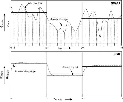
The coupling is performed with a transient decade-based LGM and a transient day-based SWAP. The output values of both models are exchanged in decades according to the model with the larger time-step, which is the LGM model. The daily output values of SWAP (qre,swa
and µswa) are transformed to decade values according to the following rules of the
time-averaging procedure (figure 2.8): − a year exists of 36 decades;
− the first two decades in a month count 10 days each;
− the third decade includes the number of days to complete the month; − the leap day has been accounted for.
The LGM model uses smaller internal time-steps to reach convergence, which is usually within a few days (figure 2.8). The output values of LGM(ϕ2,lgm and qleft,lgm) are in decades
and used as input for the bottom boundary of the daily-based SWAP model.
0 1 10 20 31 0 1 2 3Decade Day LGM SWAP qre ,s wa µswa φ2, lg m qle ft,l gm internal time-steps daily output decade output decade average
Figure 2.8. Time-averaging aspects of the coupled LGM-SWAP model. Top: Daily output of SWAP averaged to decade values for LGM. Bottom: Internal calculation time-steps of LGM used to produce decade output values, used as input for SWAP.
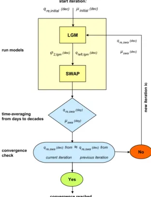
2.3.4 Convergence procedure
The coupling between LGM and SWAP is based on the following iterative procedure (fig-ure 2.9):
− run LGM with initial input series of the groundwater recharge qre,initial (m d-1) and the
a one-year period is used, with an average of 0.8 mm d and an amplitude of 0.4 mm d , the maximum value is reached at day 90. The µinitial (-) has a constant value of 0.1 (-)
dur-ing the first run. The same input series for the groundwater recharge rate and phreatic storage capacity are applied to all finite element nodes as the upper boundary condition of LGM;
− apply the decade values of the LGM-calculated groundwater heads of the second aquifer of LGM ϕ2,lgm (m) and the phreatic leftover flux qleft,lgm (m d-1) to the lower boundary
condition of SWAP and run the SWAP model;
− proceed to time averaging of the daily output of SWAP to decades values of the ground-water recharge and storage capacity;
− check whether convergence has been reached. The LGM-SWAP convergence has been reached if the groundwater recharge qre,swa (m d-1) no longer show significant changes
with the groundwater recharge from the previous iteration.
convergence reached LGM SWAP No Yes (dec) initial re, q iteration previous iteration current from q from
qre,swa(dec) ≈ re,swa(dec)
(day) swa (day) swa re, µ q (dec) swa (dec) swa re, µ q (dec) lgm left, (dec) lgm 2, q ϕ new ite ra tion ic (dec) initial µ start iteration: run models time-averaging from days to decades
convergence check
Figure 2.9. Convergence procedure of the coupled LGM-SWAP model.
2.3.5 Surface waters
As the surface waters form an important part of the hydrological functionality in both LGM and SWAP, their parameterisation should be consistent and produce practically the same drainage/infiltration fluxes. Taking in consideration the functionality and limitations of both models leads to the following approach.
Local surface waters
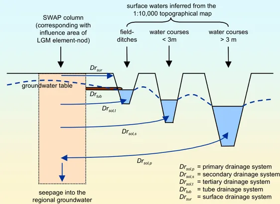
Five different local surface water systems are distinguished, in accordance with the classifica-tion in STONE (Kroon et al., 2001). In this concept, three local drainage systems are used for
the simulation of discharge into the primary, secondary and tertiary surface water systems (figure 2.10). The definition of these classes was inferred from 1:10.000 Dutch topographical maps. Out of these three systems, only the primary system can simulate infiltration, using an infiltration resistance that may differ from the drainage resistance. Preferable, but not yet possible in the applied ‘basic drainage option’ of SWAP, is to limit the infiltration rate by defining a groundwater level at which the maximum rate is reached.
field-ditches water courses < 3m water courses > 3 m SWAP column (corresponding with influence area of LGM element-nod)
surface waters inferred from the 1:10,000 topographical map
seepage into the regional groundwater Drsol,p Drsol,s Drtub Drsol,t Drsur
Drsol,p= primary drainage system
Drsol,s = secondary drainage system
Drsol,t = tertiary drainage system
Drtub = tube drainage system
Drsur = surface drainage system
groundwater table
Figure 2.10. The five local drainage systems considered in the coupled LGM-SWAP model (after Tik-tak, 2003).
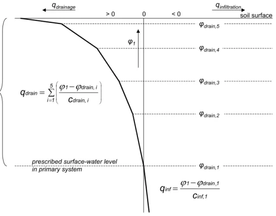
The fourth and fifth drainage systems are used for tube drainage and rapid discharge at the soil surface. This surface drainage occurs when the groundwater table is nearing the soil sur-face. Due to its irregularities the soil surface will then start to function as a drain. The surface drainage resistance has a constant value of 10 days. The lumped drainage relations of the five local surface water systems, such as they are incorporated in the coupled LGM-SWAP model, are shown in figure 2.11.
Surface runoff
In LGM the simulation of surface runoff is not possible. In SWAP on the other hand, it is a standard functionality which can not be switched off. However the consequence of this in-consistency is limited due to the introduction of the (rapid) surface drainage system, men-tioned before. Its low drainage resistance will in most cases prevent the groundwater table from reaching the soil surface.
φ1 > 0 0 < 0 qdrainage qinfiltration soil surface φdrain,5 φdrain,4 φdrain,3 φdrain,2 φdrain,1 ∑ − = = 5 1 i drain,i i drain, 1 drain c q ϕ ϕ inf,1 1 drain 1 inf c q =ϕ −ϕ ,
prescribed surface-water level in primary system
Figure 2.11. Lumped drainage relations of the five surface water systems, as incorporated in the LGM-SWAP model. The drainage-/infiltration flux is a function of the groundwater height (ϕ1),
3.
Derivation of the spatial schematisation and model
pa-rameterisation
The coupled model is applicable at both the regional and the national scale, the difference being the size of the modelled area. An example of a regional-scale application is presented in chapter 4 (modelled area 700 km2, nodal distance 500 m), while a national-scale applica-tion is discussed in chapter 5 (modelled area 31600 km2 with node distance 1250 m, locally downscaled to 250 m). The model output can be generated at any spatial resolution with dis-tances between the model nodes even as small as 25 meters, the latter distance being the most detailed resolution in input data.
3.1 Spatial schematisation
The spatial coupling of LGM and SWAP is realised by using a direct and unique parameteri-sation linkage between the two models, the so-called one-to-one spatial coupling between LGM and SWAP. In this one-to-one coupling the parameter values for both LGM and SWAP are derived for the same node influence area. Examples of influence areas are shown in fig-ure 2.1. Running the LGM-SWAP model consists of a repeated processing of LGM and SWAP (see section 2.3.4).
The advantage of the one-to-one spatial schematisation is that full consistency is guaranteed between the parameter input values for LGM and SWAP. The drawback of the one-to-one approach is a high execution time of the SWAP model. It is for this reason that –with the cur-rently available computational power– the coupled LGM-SWAP model can be used only for a limited number of nodes. In practice, however, it is often required to zoom in on some areas with a great spatial detail, such as in areas with a high hydraulic gradient, areas with a distinct variability of the groundwater table, or in areas with ecologically valuable water-dependent habitats. When dealing with a large number of model nodes, two ways can be followed: − decrease the number of SWAP runs by running SWAP only at the limited number of
so-called ‘unique combinations of SWAP plots’ (Kroes et al., 2001). Using SWAP plots im-plies a certain loss of physical relevance and, thus a decrease of accuracy of model out-puts. After all, a SWAP plot used at a certain node does not represent the actual parame-ters uniquely pertaining to that node;
− use the combined one-to-one LGM-SWAP model in combination with a downscaling procedure to generate greater spatial detail.
In this study (chapter 5) we have used the latter two-steps approach: (a) the application of a spatially coarse coupled LGM-SWAP model, with the node distance of 1.25 km and node influence area 1.3 km2, (b) followed by a single run of a spatially detailed transient LGM model (node distance 250 m) that uses as input the groundwater recharge and storage coeffi-cient downscaled from the coarse coupled model. The detailed transient LGM run is carried out only once, without feedback to SWAP. The feedback is omitted due to high computa-tional time required for running the SWAP model. Therefore its result is an approximation of
the output that would have been achieved by applying iteratively the coupled LGM-SWAP model for the detailed 250-m grid. Both LGM models in the two-step approach are identical in terms of model schematisation and parameterisation, such as the type of boundary condi-tions, layering of aquifers and aquitards, and the topsystem definition.
3.2 Parameterisation of LGM
Model parameterisation is the process resulting in the parameter values at the nodes of the model grid, further referred to as model parameters or model input values. The main type of model parameters concerns the spatially distributed parameters, for example aquifer trans-missivities and hydraulic resistance of aquitards. The other model parameters are line-based parameters (rivers) and point-based parameters (wells).
3.2.1 Spatially distributed parameters
The key element for parameterisation of spatially distributed parameters are the influence ar-eas of nodes, denoted as Ainf (m2). The influence areas are used to generate the parameter
in-put values from the basic data in ArcInfo. Three types of basic data (ArcInfo coverage) are used:
− point information like the elevation of ground level;
− line information like thickness of geological layers and hydraulic conductivity of aqui-fers;
− polygon information like the identification code of geological formations.
An example of a finite element grid for LGM is shown in figure 2.1. An influence area is a polygon. Only if the grid consists of quadrangles, the influence areas will simplify into quad-rangles.
The model parameter values at nodes can always be derived by assigning the nodal values from ArcInfo coverage. The procedures are described below in ‘Step 1, spatial parameterisa-tion’. However, this straightforward assignment method may be used only if the parameters do not significantly vary within the space of the model-node influence area Ainf. If a
parame-ter varies strongly within an influence area – which in our case is expected to occur for influ-ence areas Ainf larger than 250 x 250 m2 – then an area-weighted spatial averaging within the
influence area must be used to account for the parameter variability. The area-weighted spa-tial averaging for generation of model parameters distinguishes four steps:
− first define the parameter values at the nodes of an intermediate grid, which is finer than the model grid. In our case, the intermediate grid consists of a regular mesh of square-shaped elements, with the node distance of 250 m. For basic information defined by ArcInfo coverage for points and lines, the parameter values at the intermediate-grid nodes are defined through the TIN interpolation. For basic interpolation defined by polygons, the parameter values at the intermediate-grid nodes are defined by trivial assignment (identity function in ArcInfo);
− second, execute the existing procedures (computer programs and algorithms) to calculate the model parameters at the nodes of the intermediate grid. An example of this is the cal-culation of aquifer transmissivity as a product of the layer thickness and the hydraulic
conductivity, and the calculation of hydraulic resistance of aquitards as a function of the layer thickness, the layer depth and the type of geological formation (lithology);
− third, generate an overlay of the influence area Ainf of the model nodes with the influence area of nodes in the intermediate grid. This intersection of two sets of influence-area polygons produces another –more detailed– image of polygons, intersection polygons; − finally, as fourth step, use an averaging procedure to calculate the model input values –
parameter values at the nodes of the model grid– from parameter values previously de-fined at the nodes of the intermediate grid. An arithmetic area-weighted average for the intersection polygons is used for all parameters, with the exception of hydraulic resis-tances. In order to preserve the water balance, the area-weighted averaging cannot be done for hydraulic resistances themselves but has to be done for their inverse value.
In the remainder of this section, the basic data and the procedures are discussed regarding the spatially distributed parameters used in this study. The parameters concerned are the ground level, the boundary conditions, aquifers and aquitards, small-scale surface waters, tube drain-age, and surface drainage (in Dutch: ‘maaiveldsdrainage’).
Ground level
The spatial map of the ground level (meters above mean sea level) is based on the topog-raphic map 1:10,000. The map was digitised to a point-type ArcInfo coverage.
Boundary conditions
LGM requires as input the groundwater heads along the model periphery (constant in time) and the initial groundwater heads within the model area. The latter are the groundwater heads at the onset of the transient calculation. In the application discussed in chapter 5, the time of zero coincides with the beginning of January 1, 1986. The boundary-condition groundwater heads for each of the five aquifers were derived from TNO-NITG groundwater head observa-tions for the year 1988. The annual average for 1988 was spatially interpolated (using the TIN procedure in ArcInfo) to the nodes of the model grid.
Aquifers and aquitards
The groundwater system in the Netherlands can be described as a multi-aquifer system con-sisting of a sequence of aquifers and aquitards, where the groundwater head in the shallow phreatic top aquifer is strongly influenced by the small-scale surface water system. For the description of the groundwater flow in this system, the Dupuit assumption can be adopted for the flow in the aquifers, while the flow in the aquitards is assumed to be vertical one-dimensional. Five aquifers are distinguished –the phreatic aquifer and four deeper aquifers–, separated by aquitards, and underlain by an impervious base.
Two blocks with basic information are distinguished, namely the data for the phreatic top aq-uifer, and the data for the aquifer-aquitard system below the phreatic aquifer.
The information required for the phreatic top aquifer is contained in TNO-NITG (2002). That report documents the results of a national-scale study carried out for the topsystem layers in
the Netherlands. For this purpose, the ‘topsystem’ is conceived to be the zone of moderately-to-reasonably permeable deposits occurring (a) between the ground level and the top of the first distinctly permeable layer (to become our model aquifer 1) (b) or, if no aquifer exists within a few metres below ground level (such as in peat-clay polder areas), between the ground level and the bottom of the first-encountered semi-confined layer (aquitard 1, separat-ing the top aquifer and aquifer 2). The national-scale inventory distseparat-inguished 25 subareas, each assumed to have a homogeneous geological structure. The inventory was based on shal-low borings, and the shalshal-low section of the borings from the DINO archive of TNO-NITG (http://dinoloket.nitg.tno.nl). Using the overall information, the vertical hydraulic resistance and transmissivity of the top aquifer were derived.
For the deeper system, use is made of the geohydrological information already available in the previous version of LGM (Pastoors, 1992). Amongst other items, this database contains: − the z-level (metres above m.s.l.) of the top and the bottom of each aquifer and aquitard; − the hydraulic conductivity of aquifers;
− the relationship between the aquitard thickness and the aquitard depth, and the resulting hydraulic resistance of the aquitard. After all, the resistance does not have to be a linear function of the layer thickness. This information is spatially structured through the identi-fication code of geological formations, each formation having its own unique characteris-tics.
The transmissivity of aquifers at each model node is calculated as the product of the hydrau-lic conductivity and the aquifer thickness, the latter being the difference of z-levels at aquifer tops and bottoms. The hydraulic resistance of aquitards at model nodes is calculated as a function of the aquitard thickness and the depth of aquitard top below ground level. At places where the aquitard is lacking, the minimum value of hydraulic resistance of 10 days was adopted. More information on the parameterisation is contained in Pastoors (1992).
Small-scale surface waters
Interaction of the top aquifer (phreatic aquifer) with the small-scale surface water system (ditches, drains, brooks) is approximated by a spatially distributed source/sink, where the in-filtration or drainage is dependent on the phreatic groundwater head. This flux interaction is handled by means of the so-called topsystem flux relation, as it is described in section 2.1. The other two components of the topsystem flux relation are the tube drainage and the sur-face drainage.
The small-scale surface waters are split up into three drainage system groups, namely the primary, the secondary, and the tertiary system. This classification is based on the channel width classes used in the Top10-vector database, the topography database containing also the location of all surface waters:
− shallow trenches (small ditches) and gullies that carry water only at very shallow groundwater tables (tertiary system);
− watercourses with width smaller than 3 m (secondary system); − watercourses with width between 3 and 6 m (primary system);
− watercourses with width larger than 6 m (primary system).
Figures 3.1 and 3.2 illustrate, for a model area in the southern Netherlands, the location and density of the secondary and tertiary drainage systems. The model area shown in the figures is the Brabant-Oost submodel (discussed in chapter 5).
Figure 3.1. Example of location and density of secondary drainage systems, depicted for the Brabant-Oost submodel in southern Netherlands (for location refer to figure 5.1).
Figure 3.2. Example of location and density of tertiary drainage systems, depicted for the Brabant-Oost submodel in southern Netherlands (for location refer to figure 5.1).
The model parameters required as input for the LGM-SWAP model are (a) the drainage depth (the depth of the drain bottom or surface water below ground level), (b) the hydraulic resis-tance for the drainage condition, and (c) the hydraulic resisresis-tance for the infiltration condition. Obviously, the infiltration from a watercourse into groundwater can occur only if surface wa-ter is available and the wawa-ter level in the wawa-tercourse is maintained, as is often the case in polder areas.
For the parameterisation of the drainage depth at each model node, use is made of the so-called ‘hydrotype’ classification (Massop et al., 2000), based on the 1:600.000 geological
map of the Netherlands and geohydrological characteristics of the topsystem. A hydrotype relates to geological characteristics (history) of a region. Separate hydrotypes are defined for, for example, a clay region, a loess region, a river back-swamp region, or a glacial-till region. However, the drainage depth of existing watercourses not only relates to a hydrotype, but also to the groundwater dynamics. The latter expresses the variability of the phreatic groundwater table in time. A convenient way to classify the groundwater dynamics in the Netherlands is the Gt-value, being an identification number for the groundwater depth class (Gt-map 1:50.000). For the parameterisation, we applied the drainage depth as a combined function of hydrotypes and Gt-values (Massop et al., 2000, Appendix 2).
The parameterisation of the drainage resistance and the infiltration resistance at each model node was carried out assuming that the two resistances were equal. For convenience, in the remainder of this section we will use the term ‘drainage resistance’ to denote also the infiltra-tion resistance. The nodal value contribuinfiltra-tion of the drainage resistance, RDiw (d), due to one
watercourse segment, segment iw, within a model-node influence area follows from:
RDiw = Rbot,iw Ainf / Aiw (3.1)
where Rbot,iw (d) is the hydraulic resistance of the material at the watercourse bottom, and
Aiw(m2) is the surface area of the watercourse segment iw within Ainf. The segment area Aiw is
a product of the segment length (m) within Ainf and the segment width (m). The segment
length within Ainf follows directly from the vector database. However, as the
Top10-vector database does not include the information about the watercourse width, a national-average value of the watercourse width was construed and used for each of the three drainage system groups:
− primary system: the mean of the watercourse width assumed 5 m; − secondary system: the mean of the watercourse width assumed 2 m; − tertiary system: the mean of the watercourse width assumed 1 m.
Rbot,iw, the hydraulic resistance of the material at the watercourse bottom is not known for
each individual watercourse. For this reason, a national-average value was taken for each of the three drainage system groups:
− primary system: the mean of the bottom resistance assumed 4 days; − secondary system: the mean of the bottom resistance assumed 2 days; − tertiary system: the mean of the bottom resistance assumed 1 days.
Tube drainage
A considerable part of the surface area of the Netherlands is drained by tubes and tiles, espe-cially in clayey areas. Little information is available about the location of tubes and tile drains. For the parameterisation, use is made of the tube drainage location map from the STONE project (Massop, 2002). This map was prepared using rules of thumb expressing the probability of tube drainage occurrence at various combinations of land use and the ground-water depth class (Gt-value), supplemented by expert judgement. The drainage resistance of
tubes is assumed spatially constant, at the value of 100 days. Also the tube depth is assumed spatially constant, at 1 m below ground level.
Surface drainage
The ground surface is not even, being variable in space (dips and tops, relief on macro- and micro scale). The degree of ground surface deviation from an ideal even (flat) surface in-creases with the size of the model-node influence area Ainf increasing. As the phreatic
groundwater level starts approaching the ground surface, the relief in ground surface start col-lecting surface water and carrying this surface water to drains and ditches. In other words, the ground surface functions as if it were a drain/ditch system. The resistance of the surface drainage is assumed spatially constant, at the value of 10 days. Also the drainage depth is as-sumed spatially constant, at 0.2 m below ground level.
3.2.2 Rivers and canals
As is considered in section 2.1, LGM features two options for the interaction with surface waters, namely the topsystem-flux relation, to account for the small-scale surface waters, and the so-called rivers. The rivers represent large (wide) river courses such as the Rhine River and its major branches (IJssel River, Waal River, etc.), the Meuse River, and various canals (Amsterdam-Rhine Canal, Twente Canal). The centre line of those large water bodies was incorporated as element sides in the finite element grid (figure 3.3). The parameterisation of rivers/canals was based on the data from the previous version of LGM (Pastoors, 1992). The relevant parameters are the river width, and the drainage and infiltration resistance of the river bottom.
Figure 3.3. Location of rivers and canals incorporated as nodes in finite-element grid for national-scale LGM-SWAP Modelling.
It is worthwhile mentioning here that rivers and canals serve as an internal boundary condi-tion of the Cauchy type. Due to the large porcondi-tion of surface water area it will not be meaning-ful to carry out SWAP calculations at those model nodes.
3.2.3 Wells
The groundwater abstractions consist of abstractions for drinking-water supply and abstrac-tions for industrial purposes. The LGM-SWAP calculaabstrac-tions were carried out for a single ideal well location for each abstraction site. In reality, the abstraction for drinking-water produc-tion takes place in most cases by means of a series of wells spread over a certain area. The well locations, assumed in the ‘ centre of gravity’ of the real well locations, are specified in-dependently of the finite-element grid, i.e. they can be located anywhere inside the grid ele-ments. The program automatically allocates the groundwater abstraction rates to the grid nodes composing the element in which an abstraction site is located. The parameterisation of groundwater abstractions was based on the data from the previous version of LGM (Pastoors, 1992). The well rates from this database represent the amount of groundwater abstracted in 1988.
3.3 Parameterisation of SWAP
To avoid data redundancy, a relational database was set up to assign the parameter values for all SWAP-plots (figure 3.4) This database contains a hierarchy. At the highest level, a dis-tinction is made between spatially constant parameters and spatially distributed parameters. The spatially distributed parameters are given at the plot level. At this level a subdivision is made between spatially distributed parameters that are part of the model parameterisation and those forming a part of the iteration procedure of LGM-SWAP. The latter are parameters al-tered during each iteration of LGM-SWAP. These parameters mainly concern the time-variable parameters for the Cauchy bottom boundary condition. Prior to each SWAP run it is determined whether the Cauchy condition or the free drainage condition will be applied for the bottom boundary. The free drainage option will be used in case the groundwater remains 6 m below the soil surface, during the entire simulation period of LGM.
A good estimation of the initial groundwater level at the start of a simulation by SWAP will reduce the adjustment period of the calculations considerably. Therefore the initial groundwa-ter level used as input, is the average groundwagroundwa-ter level calculated by the previous run of LGM.
Certain spatially distributed parameters that are part of the model parameterisation are valued in accordance with the model parameterisation of LGM. Parameter values for the drainage characteristics and the hydraulic resistance of the bottom boundary layer (the uppermost aqui-tard) are assigned to each individual plot. The remaining spatially distributed parameters are related to three basic parameters, namely the soil profile number, the weather district and land-use type.
Spatially distributed variables Assessment Plot ID Start date End date Output control Meteo district Rainfall Temperature ETref Soil profile Soil layer ID Land-use Emergence date Harvest date Development stage ID Critical pressure heads for drought stress and irrigation Development stage LAI Crop factor Rooting depth Soil layer
Soil physical unit ID Layer thickness
Soil physical unit Parameters of the Mualem-van Genuchten functions Plot Weather district ID Land-use type ID Soil profile ID Drainage characteristics Irrigation switch Resistance for Cauchy bottom boundary condition
Plot
Time-variable parameters for Cauchy bottom boundary condition Free drainage switch Initial groundwater level
Parameters altered during iteration
Figure 3.4. Simplified scheme of the GeoPEARL database (only hydrology), used for running multiple SWAP-plots (after Tiktak et al., 2003).
To determine the values of these three basic parameters a map overlay with the finite element grid of LGM has been carried out. The assigned ID’s of each of the three parameters is the dominant value within an influence area of a node. By that the influence areas, belonging to the nodes of the finite element grid, are normative for defining the parameter values for SWAP.
Time series of precipitation, temperature and reference evapotranspiration according to Mak-kink (1957) were available for 15 weather stations. Each station was assumed to be represen-tative for an entire weather district, together covering the total area of the Netherlands. The map is based on an allocation of the weather stations to PAWN-districts, according to Kroes et al. (1999). For 14 weather stations only decade values of precipitation, temperature and reference evapotranspiration were available. However daily observations of these meteoro-logical parameters were available for the weather district De Bilt. To obtain daily values for all weather stations the daily variation of the observations of De Bilt has been superimposed on the decade values of the other stations.
Three crop types were distinguished for the simulation of evapotranspiration, namely perma-nent grassland, maize and other arable land. The areas covered with these three crop types are determined by means of a classification of the land-use map LGN3+ (De Wit et al., 1999). Emergence date, harvest date and development stage dependent crop parameters were derived from simulations with a crop growth model (Hijmans et al., 1994). Critical pressure heads for
drought stress (and irrigation) were taken from Van Dam (2000). So far irrigation has been switched off.
There are 21 soil profiles distinguished, which are derived from the soil map 1:50.000 (Klijn, 1997). The applied derivation is based on the classification used to translate the 1:250.000 soil map in soil profiles (Wösten et al., 1988). Each soil profile is composed of soil horizons for which soil physical units are assigned to. Parameter values for the Mualem-Van Genuch-ten functions to describe the soil physical properties were taken from WösGenuch-ten et al. (1994).
4.
Performance of the coupled model at the regional scale
4.1 Introduction
During the development of the combined LGM-SWAP model, a small study area near Lo-chem (100 km2) was used for testing. Results of this application were described by Stoppe-lenburg et al. (2002). Following this application, the model was applied to a slightly larger catchment. The objectives of this regional modelling study were:
1) to evaluate the performance of the combined LGM-SWAP model for regional scale stud-ies. An important aspect of the performance of the combined model was the ability of both models to simulate the dynamics of the phreatic aquifer in a consistent way. There-fore, we focussed on the resulting water balances and groundwater dynamics.
2) to compare the performance of the combined LGM-SWAP model with the performance of other models. To achieve this, RIVM participates in the so-called ‘Dutch working group on hydrological modelling’. Other partners in this working group were Alterra and RIZA.
The study was carried out in the Beerze-Reusel catchment, which has a surface area of ap-proximately 700 km2. As a starting point for the study, an existing model of this catchment was used (Van Walsum et al., 2002). To facilitate the comparison between the three models, the schematisation and parameterisation were simplified (see section 4.3). Because of these simplifications, it is not possible to compare the simulated groundwater dynamics with ob-servations; the modelling study was purely performed to test consistency between the models and not to test validity of the final model.
This chapter continues with an introduction to the study area (section 4.2), followed by a short description of the model set-up (section 4.3). In section 4.4, the convergence of the coupled LGM-SWAP model is discussed. The performance is discussed in sections 4.5 and 4.6, respectively on regional level and on plot level. Conclusions are given in section 4.7.
4.2 Description of study region Beerze-Reusel
The study region is located in the Province of Noord-Brabant in the southern part of the Netherlands (figure 4.1). An overview of the Beerze-Reusel catchment itself is depicted in figure 4.2. The description of the study region is partly based on Van Walsum et al. (2002). The subsoil consists mainly of sandy deposits formed in the Pleistocene. The region gently slopes in a north to north-east direction, from an altitude of 45 metres above mean sea level (m above m.s.l.) down to approximately 4 m above m.s.l.. There are several aeolian sand ridges several meters high, orientated in west-east direction. These ridges have a large impact on the geomorphology of the stream valleys, as they are situated transversely to the general slope and drainage pattern of the area. In those areas where the rivers traverse the sand ridges, the valleys narrow, sometimes to no more than a few tens of metres. In the plains between the
ridges the valleys are wider. In the valleys, alluvial soils have formed, consisting of rede-posited sand, loam and peat. Because of the intensive agricultural drainage these peat soils are strongly oxidised and have often become very thin.
N
Study region
Large cities in Province of Noord-Brabant Boundaries of provinces Eindhoven 's-Hertogenbosch Tilburg Breda 10 0 10 20 Kilometers
Figure 4.1. Location of the study region in the southern part of the Netherlands (Van Walsum et al., 2002).
Agriculture is the dominant land use in the region. Most of the area is used for grassland and maize. In the region there are a few larger nature conservation areas of more than 1000 ha. These areas are mainly situated on the higher aeolian sand ridges and consist of heathland and pine plantations. The nature conservation areas in the stream valleys are less numerous and are generally much smaller, sometimes not bigger than a few hectares.
4.3 Model set-up
Model set-up follows the generally applicable method as described in detail in chapter 3. However, as described in section 4.1, the existing model (Van Walsum et al., 2002) was sim-plified for this particular study. The most important simplifications were:
− the number of aquifers was reduced from seven to four;
− the groundwater heads along the model periphery were taken from the NAGROM-model; − only the three largest groundwater abstractions were input into the model;
− tube drainage was assumed at a constant depth of 90 cm below ground level; − a constant tube-drainage resistance of 100 days was assumed;
− the entire area was assumed to be covered by grassland; − the root-zone depth was fixed at 30 cm below ground level;
− the number of weather districts was reduced from five to one (district-number 13 ‘Ge-mert’).