QMRAspot: a tool for quantitative microbial risk assessment for drinking water : Manual QMRAspot version 2.0

(1)

RIVM report 2014-0020

J.F. Schijven et al.

(2)

(3)

QMRAspot: a tool for quantitative

microbial risk assessment for drinking

water

Manual QMRAspot version 2.0 RIVM Report 2014-0020

(4)

Colophon

Parts of this publication may be reproduced, provided acknowledgement is given to: National Institute for Public Health and the Environment, along with the title and year of publication.

This is a publication of:

National Institute for Public Health and the Environment

P.O. Box 1│3720 BA Bilthoven The Netherlands

www.rivm.nl/en Jack Schijven

,

RIVM Saskia Rutjes

,

RIVM

Patrick Smeets

,

KWR Watercycle Research Institute Peter Teunis

,

RIVM

Contact: Saksia Rutjes Z&O

Saskia.Rutjes@rivm.nl

This investigation has been performed by order and for the account of the Ministry of Infrastructure and the Environment, within the framework of the Knowledge Base Drinking Water (project number M/300005/01/CA)

(5)

Abstract

Manual for QMRAspot, a computational tool for the assessment of quantitative microbial risks of drinking water consumption.

The RIVM has developed a user-friendly computational tool (QMRAspot) to calculate the risk of becoming infected by pathogenic microorganisms in drinking water. This report is a manual in which it is explained how QMRAspot

(Quantitative Microbial Risk Assessment from surface water to potable drinking water) can be used, and what the underlying models are. The tool is mainly aimed at pathogenic microorganisms in drinking water produced from surface water. The manual applies to the most recent tool version (2.0, September 2014).

The Dutch drinking water companies that produce drinking water from surface water and groundwater are obliged by law to demonstrate that less than one per then thousand persons per year acquire an infection by consumption of unboiled drinking water. QRMAspot was originally developed for the Netherlands, but can be applied worldwide by drinking water companies, researchers and policy makers.

This manual describes in detail how data for the risk assessments can be provided, how these data are analysed statistically, and how the risk assessments can be conducted in a consistent and transparent manner. In addition, two frequently occurring applications of QMRAspot are discussed. The first application demonstrates the effect on the infection risk of a high

contamination at locations where the drinking water companies abstract surface water. The second application demonstrates to what extent one single sample, in which microorganisms were detected, contributes to the infection risk. Keywords: Quantitative Microbial Risk Assessment; tool; drinking water; index pathogen

(6)

(7)

Publiekssamenvatting

Handleiding voor QMRAspot, een rekenprogramma voor het schatten van kwantitatieve microbiologische risico’s van drinkwater.

Het RIVM heeft een gebruiksvriendelijk computerprogramma (QMRAspot) ontwikkeld dat de kans berekent op infecties door ziekteverwekkende micro-organismen in drinkwater. Het onderhavige rapport is een handleiding, waarin wordt uitgelegd hoe QMRAspot (Quantitative Microbial Risk Assessment from surface water to potable drinking water) gebruikt kan worden en wat de onderliggende rekenmodellen zijn. Het model is voornamelijk bedoeld voor ziekteverwekkende micro-organismen in drinkwater dat uit oppervlaktewater wordt gewonnen. De handleiding is van toepassing op de meest recente modelversie (2.0, september 2014).

De Nederlandse drinkwaterbedrijven, die drinkwater produceren uit

oppervlaktewater en grondwater, zijn wettelijk verplicht om aan te tonen dat minder dan één op tienduizend personen per jaar een infectie oploopt door de consumptie van ongekookt drinkwater. QRMAspot is oorspronkelijk ontwikkeld voor Nederland, maar kan wereldwijd worden toegepast door

drinkwaterbedrijven, onderzoekers en beleidsmakers.

In deze handleiding wordt in detail beschreven hoe gegevens voor de

risicoschattingen kunnen worden aangeleverd, hoe deze gegevens statistisch worden geanalyseerd en hoe de risicoschatting op consistente en transparante wijze kan worden uitgevoerd. Ook worden twee veel voorkomende toepassingen van QMRAspot besproken. De eerste toont het effect op het infectierisico van een hoge besmettingsgraad op locaties waar de drinkwaterbedrijven het

oppervlaktewater onttrekken. De tweede toepassing demonstreert in welke mate één enkel monster waarin micro-organismen zijn aangetoond, bijdraagt aan het infectierisico.

Kernwoorden: Kwantitatieve microbiologische risicoschatting; tool; drinkwater; indexpathogeen

(8)

(9)

Summary

QMRAspot is an interactive computational tool that has been designed for conducting Quantitative Microbial Risk Assessment (QMRA) for drinking water produced from surface water. This manual explains how to use QMRAspot as well as the underlying models in detail. QMRA results are explained on the basis of a reference data set. An example with the effect of a peak concentration in the source water and an example with treatment data consisting of only non-detects or only one positive sample in the effluent of the treatment step are shown. The manual applies to QMRAspot version 2.0 (1/9/2014).

In the Netherlands, drinking water companies are legislatively obligated to demonstrate compliance to not exceeding an infection risk of one per ten thousand persons per year from consumption of drinking water. This has to be demonstrated every four years for four index pathogens: Enterovirus,

Campylobacter, Cryptosporidium and Giardia. QMRAspot has been designed to

conduct QMRA for these index pathogens.

This report explains how QMRAspot assesses the infection risk and addresses possible applications. A comprehensive description of QMRAspot version 1.0 has been published by Schijven et al. (2011), which is fully cited in this manual, supplemented with explanation in more detail and examples, and updated to version 2.0 of QMRAspot. QMRAspot was originally developed in Mathematica 8.0.4 (Wolfram, Inc, Champaign IL, USA). The current QMRAspot version 2.0 has been updated to run with version 9.0.1 of Mathematica, Player Pro and CDF Player. QMRAspot version 2.0 has been extended to include a fifth optional pathogen, distribution parameter values for recovery can be set by the user, a dose response model can be selected, and dose response parameter values can be set by the user for the fifth pathogen. Raw data for QMRA to estimate the concentration of pathogens in the source water and to estimate removal of pathogens and/or indicator microorganisms by drinking water treatment must be stored in an Excel spreadsheet. These data can be read by QMRAspot with Mathematica or Player Pro. QMRAspot fits distributions to these data. In addition and/or instead, distribution parameter values can be set interactively in

QMRAspot. A QMRA can thus be conducted without analyzing raw data as well. With the free CDF Player, data cannot be read from a spreadsheet, but QMRA can still be conducted by setting parameter values.

A QMRA report can be generated for each of the index pathogens, and this report can be saved as a Mathematica notebook and/or pdf file.

(12)

(13)

1 Introduction

1.1 Drinking water legislation

The World Health Organization (WHO) Guidelines for Drinking Water (WHO 2011) outline a preventive management framework for safe drinking water entailing health based targets, system assessment from source through treatment to the point of consumption, operational monitoring of the control measures in the drinking water production, management plans documenting the system assessment, and monitoring plans and a system of independent

surveillance that verifies that the above are operating properly.

In line with the WHO Guidelines, the Dutch Drinking Water Act (2009) prescribes that tap water provided by the owner to consumers and other customers should not contain micro-organisms, parasites or substances to such numbers per volume or concentrations that these may comprise detrimental public health effects (Article 21). In the Dutch Drinking Water Act (2011), this demand is translated into the following quality requirements:

1) Absence of E. coli and enterococci in 100 ml of drinking water;

2) (Entero)viruses, Cryptosporidium, Giardia and Campylobacter should not exceed an infection risk of one infection per 10,000 individuals per year. In the Dutch Drinking Water Act (2011), no specific directions are given on how to perform this so-called Quantitative Microbial Risk Assessment (QMRA). To guide the owner of the provided tap water and the Inspectorate body on how to perform QMRA, the Inspectorate Guideline 5318 (Anonymous, 2005) was drafted in close consultation between the government (Environmental Inspectorate), the National Institute of Public Health and the Environment (RIVM), Bilthoven, the Netherlands, and the drinking water producers. The general principle of the Inspectorate guideline is to balance health protection and public funds.

1.2 General explanation of QMRA

The required quantitative risk assessment is based on source water quality and the efficiency of the applied treatment. In addition, data are needed concerning tap water consumption and the dose-response relation of the specific pathogen and its host. Risk assessment for exposure to pathogenic microorganisms in drinking water was described by Teunis et al., 1997, Haas et al., 1999 and Haas and Eisenberg, 2001, the ILSI framework (Benford, 2001) and Medema et al.

(14)

production volume (Anonymous, 2005). In addition to regular monitoring, a number of incidental samples must be collected at moments when peak concentrations in pathogen counts are assumed to occur, for example due to heavy rainfall.

Because treatment efficiency is commonly highly location specific, treatment data should be collected at every production location. Any changes in the

treatment process require a new estimation of the treatment efficiency, and thus new collection of data. Commonly, pathogen concentrations decrease below detection limits as a result of drinking water treatment. Therefore, indicator organisms are used to characterize treatment. They have similar properties as the index pathogens, and are assumed to be removed equally or less efficient by drinking water treatment. Appropriate indicator organisms occur in higher numbers and are easier to enumerate with higher recovery. Inspectorate Guideline 5318 (Anonymous, 2005) prescribes F-specific or somatic

bacteriophages as the indicator organisms for determining removal efficiency by drinking water treatment of enterovirus. Escherichia coli is used as the indicator organism for Campylobacter, and spores of sulphite reducing clostridia (SSRC) are used for both Cryptosporidium and Giardia.

Because the efficiency of treatment varies in time, a sampling period should therefore be sufficiently extensive and frequent to be able to account for the most important sources of variation and should take changes in treatment into account. This also holds true for changes in the source water quality and changes in the scientific knowledge into the efficiency of treatment processes. Source water quality data need to be collected on a regular basis because of possible trends and year-to-year variations. Inspectorate Guideline 5318 (Anonymous, 2005) prescribes three year data collection for source water quality.

In order to automate the QMRA process, the interactive user-friendly computational tool, QMRAspot, was developed to conduct QMRA for drinking water produced from surface water. No extensive prior knowledge about QMRA modeling is required by the user, because QMRAspot provides the user with guidance on the quantity, type and format of raw data, and performs a

statistical analysis of the raw data and then calculates a risk metric for drinking water consumption that can be compared with other production locations, a legislative standard, or an acceptable health based target. The uniform approach promotes proper collection and usage of raw data, warrants quality of the risk assessment, and improves efficiency, i.e., less time is required. QMRAspot facilitates QMRA for drinking water suppliers worldwide. The tool aids policy-makers and other involved parties in formulating mitigation strategies, and prioritization and evaluation of effective preventive measures as integral part of water safety plans.

This report explains how QMRAspot assesses the infection risk and addresses typical applications. A comprehensive description of QMRAspot version 1.0 has been published by Schijven et al. (2011), which is fully cited in this manual, supplemented with explanation in more detail and examples, and updated to version 2.0 of QMRAspot. QMRAspot was originally developed in Mathematica 8.0.4 (Wolfram, Inc, Champaign IL, USA). The current QMRAspot version 2.0 has been updated to run with version 9.0.1 of Mathematica, Player Pro and CDF Player. QMRAspot version 2.0 has been extended to include a fifth optional pathogen, distribution parameter values for recovery can be set by the user, a dose response model can be selected, and dose response parameter values can be set by the user for the fifth pathogen. Raw data are stored in an Excel spreadsheet that can be read by QMRAspot with Mathematica or Player Pro. QMRAspot fits distributions to these data. In addition and/or instead, distribution parameter values can be set interactively in QMRAspot. A QMRA can thus be

(15)

conducted without analysing raw data as well. With the free CDF Player, data cannot be read from a spreadsheet, but QMRA can still be conducted by setting parameter values.

A QMRA report can be generated for each of the index pathogens and this report can be saved as a Mathematica notebook and/or pdf file.

(16)

(17)

2 Excel spreadsheet with raw data

2.1 Raw data

For a QMRA, it is essential to collect quantitative microbial data as raw unprocessed data. Raw data on enumerated microorganisms in water are the counted numbers of the microorganisms as well as the corresponding

investigated volume of the sample. Commonly, counts are numbers of plaque-forming units (pfu) for viruses and colony-plaque-forming units (cfu) for bacteria (Schets et al., 2008; Teunis et al., 2005a). Oocysts of Cryptosporidium and cysts of Giardia may be counted manually or automatically under a microscope using fluorescent dye (Schets et al., 2008). Raw presence/absence data are presence or absence of microorganisms in replicate dilutions of a water sample (De Roda Husman et al., 2009).

Obviously, the concentration of, for example, 1 pathogen particle in 1 millilitre of water is the same as a 100 particles in 100 millilitres of water, but 100 counted particles produce a more accurate concentration estimate than just one counted particle, hence it is essential to use counts and sample volumes as they were observed, and not concentrations (ratios of count/volume).

All raw data must include a sample date, which is needed to enable plotting time-series of the data. These plots may reveal variations, trends and extreme values, and may aid making selections of the data for QMRA in the spreadsheet.

2.2 Source water data

Source water data are raw data of index pathogens in the source water (e.g. Rutjes et al., 2009; Lodder et al., 2010). At many production locations, river water first passes a storage reservoir prior to further treatment. For enterovirus, river water may appropriately be designated as source water, because human contamination in a storage reservoir is not expected. For Campylobacter,

Cryptosporidium and Giardia, the storage reservoir should be considered the

starting point of the QMRA, because of contamination of the storage reservoir water with these pathogens from birds, wildlife, or runoff from agricultural land.

2.3 Recovery data

In order to determine the recovery efficiencies of the detection method for index pathogens, ideally, each sample of source water, or a fraction used for analysis, is spiked with a sufficiently high number of, for example, a specific type of indicator organism. The spiked and recovered numbers can then be used to

(18)

2.5 QMRAdata.xls

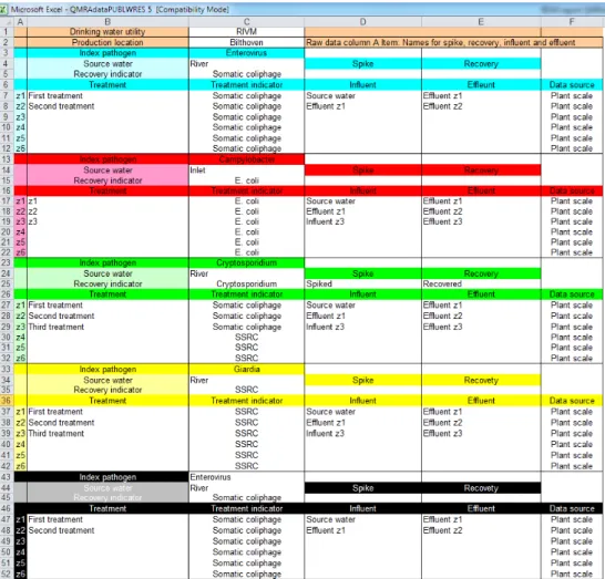
The tool reads the raw data from a standard Microsoft Excel spreadsheet file, here, for convenience, called QMRAdata.xls. It contains three sheets: SCHEME, RAW DATA and HELP. The SCHEME sheet provides a description of the drinking water production location and defines a table with column headers that is used by the tool to make the appropriate data selections. Through the SCHEME sheet, the user has control over what data should be used for QMRA. Obviously, the RAW DATA sheet contains all raw data and the HELP sheet provides background information on how to fill the RAW DATA sheet with raw data in the required format.

(19)

In the SCHEME sheet, the effluent data of a treatment step can be the influent data for the next treatment step. The data for the next treatment step may also be from other types of microorganisms, or from a different location in the drinking water utility, or from pilot plant experiments.

It is easy to modify the SCHEME sheet. For example, two treatment steps (designated z1, z2) may be combined into a single one by using the influent data of the first of the two and the effluent data of the second of the two treatment steps; in this example, z1+z2 with the influent of z1 and the effluent of z2. This can be done for each index pathogen independently.

The SCHEME sheet is a form in which the names of the drinking water company, the production location, and the names of the treatment steps can be given. Also, the names or labels for the influent and effluent of each treatment step need to be given.

The names of the source water and of the influents and effluents need to be exactly the same names as in column A Item in RAW DATA. QMRAspot uses these names for selecting the associated data.

The source of the data for the treatment steps can be selected from the following list: Plant scale, pilot plant scale, laboratory scale, and literature. Location-specific plant scale data are generally preferred, followed by pilot plant scale data, and if these are not available, data from laboratory experiments. In other words, location specific data are recommended. If the use of data from other locations is desired, applicability should be verified by comparison of treatment conditions. References to data from literature should be listed in the accompanying QMRA reports. How data from literature can be entered is described in chapter 5.

The SCHEME includes the four index pathogens Enterovirus, Campylobacter,

Cryptosporidium and Giardia. By default, the corresponding indicator organisms

for recovery are F-specific RNA bacteriophages or somatic coliphages for Enterovirus, E. coli for Campylobacter and SSRC (Spores of Sulphite Reducing Clostridia) for Cryptosporidium and Giardia, but other (arbitrary names of) microorganisms are also possible.

The names of the index pathogens and indicator microorganisms for recovery and treatment in RAW DATA column C Microorganism need to be exactly the same as given in SCHEME, so that QMRAspot can select the associated data. In version 2.0 of QMRAspot, a fifth optional pathogen can be added, for which dose-response data can be entered interactively (see section 5.6). This can be any pathogen. QMRAspot version 2.0 retains the ability to read older

(20)

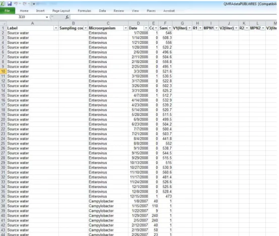
Figure 2.2 RAW DATA sheet of QMRAdata.xls

In the RAW DATA sheet, every row is a full record of raw data. This simple design allows for automated filling from a Laboratory Information Management System (LIMS), for example, as records are stored in the form of Comma Separated Values (CSV).

 Column A Label: The name of source water, "Spike", "Recovered", treatment influent, or treatment effluent.

 Column B Sampling code: Specific code. Not used in QMRA calculation, but included in RAW DATA to allow for more detailed reference. Different codes may be included for different sampling points of the same effluent. In the QMRA these are combined.

 Column C Microorganism: Index pathogens and indicator microorganisms. Exactly the same names as given in SCHEME.

 Column D Date: Date format: DD-MM-YYYY.

 Column E Count: Only positive integers are allowed. Max counts per plate according to standard method. Viral counts are counts of enterovirus or bacteriophage plaques. Bacterial counts are colony counts in detection methods for bacteria using membrane filtration. Protozoal counts are microscopic (automated) counts of fluorescent labelled (oo)cysts.

 Column F Sample size: Dimension liter. The original equivalent volume of the sample that the detected microorganisms were counted in.

Example 1: a 10-litre sample was collected, concentrated to 100 ml, 5 ml was plated for counting, then the sample size is 10/20=0.5 litre.

Example 2: 98 colonies were counted on a plate with 1 ml sample and 11 colonies were counted in the ten-fold dilution. Count is 109 and sample size is 0.0011 litres.

(21)

 Columns G-O: MPN data, Most Probable Number data. May be available instead of counts and sample volumes.

V1, V2, V3, V4, V5 are the sample volumes of five dilution steps. Dimension is litre.

R1, R2, R3, R4, R5 are the numbers of replicates for each dilution step. Only whole numbers allowed.

MPN1, MPN2, MPN3, MPN4, MPN5 are the numbers of positive samples of a particular analysed volume. Only whole numbers from 0 - the number of replicates are allowed.

Example

V1(liter) R1 MPN1 V2(liter R2 MPN2 V3(liter) R3 MPN3

0.001 3 3 0.0001 3 2 0.00001 6 4

In this example, the volume of dilution step 1 is 0.001 litres and it is replicated three times. Of those replicates, all three showed positive detection.

Recovery: RAW DATA of "Spiked" and "Recovered" microorganisms. The label is "Spike" or "Recovered". The data are counts and sample sizes.

Treatment: In SCHEME, the name of the treatment step can be given. This may also be a combination of treatment steps.

(22)

(23)

3 Run screen QMRAspot

3.1 Run

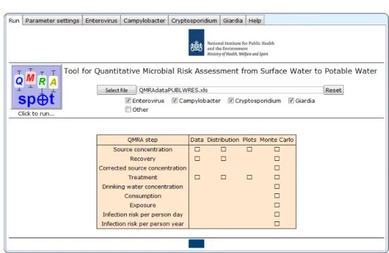
Figure 3.1 Run screen of QMRAspot at start up

At start up, the Run screen of QMRAspot has no file selected; the index pathogens Enterovirus, Campylobacter, Cryptosporidium and Giardia are all selected. Obviously, QMRAspot only conducts QMRA for the index pathogens that are selected.

Pressing the “Reset” button resets QMRAspot to this state. Resetting is disabled while QMRAspot runs.

Should a user want to stop a run of QMRAspot by aborting an evaluation, it is recommended to restart with a new kernel or reloading of QMRAspot.

(24)

3.2 Select QMRA data spreadsheet

Figure 3.2 Run screen of QMRAspot after selecting spreadsheet with QMRA data

The “Select file” button allows the selection of a QMRAdata spreadsheet. In this case QMRAdataWRES.xls has been selected. This spreadsheet contains a combination of data from several drinking water companies (Schijven et al., 2011). This particular data set can be used as the reference data set. It serves as a template for other QMRA data sets and can be used to compare QMRA outcomes calculated by different versions of QMRAspot to identify possible differences. Together with QMRAspot, each new user should have a copy of the reference data set.

(25)

3.3 Run QMRA

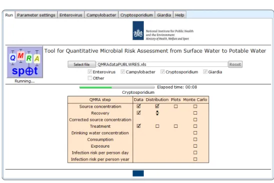
Figure 3.3 Run screen of QMRAspot at fitting distributions

The QMRAspot logo is a button. Pressing it starts the QMRA run. On the start-up screen, a progress bar allows the user to monitor that after a few seconds, QMRAspot has read all the data on source water concentration, recovery and treatment from the spreadsheet and is fitting the appropriate distribution to the data of each QMRA step.

(26)

3.4 Data analysis

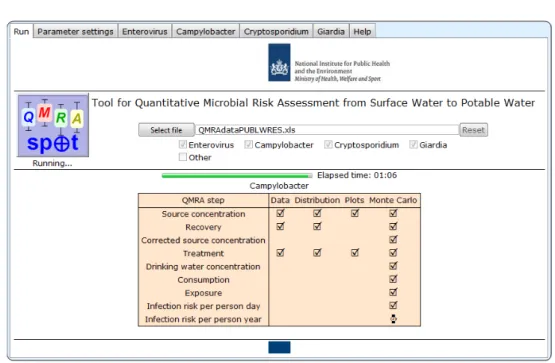
Figure 3.4 Run screen of QMRAspot almost finished

After a short while (in this case 1 minute and 6 seconds), QMRAspot has finished fitting distributions, plotting time series of the data read from the spreadsheet, drawing samples from the fitted distributions (for Monte Carlo calculations), and overall treatment, exposure and infection risks have been calculated.

(27)

3.5 End of run

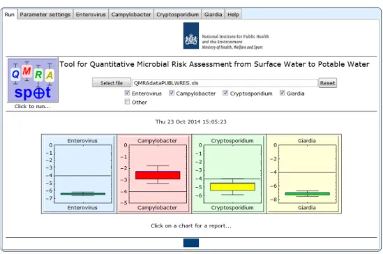
Figure 3.5 Run screen of QMRAspot at end of run

After finishing all the calculations, the main QMRAspot screen shows box-whisker plots of estimated infection risks per person per year for the selected index pathogens. The y-axis shows the infection risk per person per year on a log10 scale. The whiskers of the box-whisker plots are the 5- and 95-percentile

values of the infection risk, and the box entails the 25- and 75- percentiles. The (arithmetic) mean infection risk is indicated with a blue line. The calculated risk is presented in relation to the Dutch health target of 10-4_{per person per year. If}

the mean AND the 95-percentile lie below 10-4_{per person per year (indicated as}

a black horizontal line) then the box is coloured green to denote compliance with the health based target. The box is orange if the mean OR the 95-percentile exceeds the target. If the box is red, then the mean infection risk AND the 95-percentile exceed the target. If the 95-percentile of the infection risk is lower than 10-9_{or higher than 0.9, a message appears with this information instead of}

a box-whisker plot.

Note that a proper risk assessment outcome needs to include a risk value and its probability. In this QMRA, the mean infection risk does not fulfil that

(28)

3.6 Report

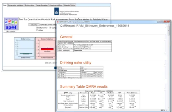
Figure 3.6 Run screen of QMRAspot at end of run with QMRA report for enterovirus in a new window.

The box-whisker plots on the run screen that appear at the end of the run are buttons that when pressed open a window with a QMRA report of the selected pathogen. The report, or selections in the report can be printed and saved as pdf.

Each report contains a general table with reference to the tool version, run date, QMRA data Excel file and which index pathogen. A drinking water utility table gives a summary description of the drinking water production location. The summary table and all histograms are included.

(29)

4 Results: Tabs with index pathogen names

4.1 General

Under the tabs with the index pathogen names the result of all the steps in the QMRA show up in detail as soon as they are available.

In the different stages of the QMRA, histograms of ten thousand Monte Carlo simulated data are presented; see section 8 for a brief explanation of Monte Carlo simulation. Ten thousand Monte Carlo samples have empirically been found to be a sufficient number of samples for a stable outcome (Teunis and Havelaar, 1999).

Figure 4.1 shows a histogram of Monte Carlo data as an example. These data are Monte Carlo samples that were drawn from a Beta distribution with parameters α=0.24 and β=970, and represent ten thousand fractions of microorganisms passing a treatment step. The left histogram shows the

probability distribution of the fractions. As can be seen, most of the fractions are very small values; therefore, a log10 transformation of the fractions is

appropriate. The left histogram shows the probability distribution of the log10

-transformed fractions from the 1- percentile to the 99-percentile. To the right of this histogram is a table presenting information on the type of distribution, distribution parameter values and some obvious statistics. Note that this distribution spans a large range. Values of -8 log10 or lower are in fact of

numbers near zero, all with a small probability.

(30)

4.2 Data scheme

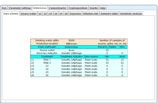
Figure 4.2 Enterovirus-Data scheme

Under Enterovirus-Data scheme, a summary table is shown of all data that were read from the spreadsheet. It shows the names of the source water and

treatment steps, and from what indicator organism treatment data were

available. The rightmost two columns show the numbers of samples available for each QMRA step.

(31)

4.3 Source water

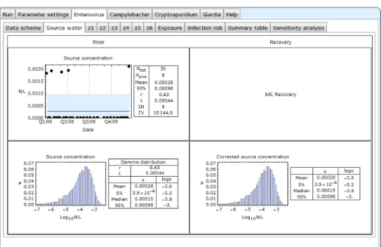
Figure 4.3 Enterovirus-Source water, no recovery data

Under Enterovirus-Source water, the source water data are presented. The top left plot shows all individual pathogen concentrations in the source water as a time series. In this particular example, in five samples (#pos) of 35 samples (#tot), enterovirus was detected. The blue line is the mean concentration of the fitted Gamma distribution for the pathogen concentration. The area shaded in light blue encompasses the area below the 95-percentile of the fitted Gamma distribution data. In five cases, corresponding to the positive samples, the estimated concentrations appear to exceed the 95-percentile value. By

definition, these values may be considered to be peak concentrations for which it is recommended investigating what environmental conditions may explain the occurrence of these high values, if not already known. N and V represent the total count and sample volume.

The bottom left panel shows a histogram of ten thousand Monte Carlo values (see also section 8) that were drawn from the fitted Gamma distribution that describes the variability of the pathogen concentrations in the source water, and a table with parameters r and λ, and some statistics of that distribution.

(32)

4.4 Source water with recovery correction

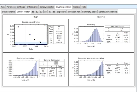
Figure 4.4 Cryptosporidium-Source water with recovery data

This screen shows the source water data for Cryptosporidium including recovery data. The recovery data encompass paired data of spiked and recovered

numbers of microorganisms to which a Beta distribution with parameters α and β is fitted. A Beta distribution describes a variability of a fraction, i.e. a number between 0 and 1. The top right panel shows the fitted distribution as a

histogram of ten thousand Monte Carlo samples. The ten thousand random samples from the Gamma distributed pathogen concentration in the source water (bottom left panel) is divided by the ten thousand random Beta distributed recovery fractions, to produce ten thousand corrected source water

concentrations, shown in the bottom right panel, as a histogram and a table with a few statistics; see section 8 for a brief explanation of Monte Carlo simulation. The distribution of the corrected concentration has shifted approximately one log10 to the right and is a bit wider than the distribution of the source

(33)

4.5 Treatment z1

Figure 4.5 Enterovirus-z1, the first treatment step “Step 1”

Enterovirus-z1 shows influent and effluent somatic coliphage concentrations of the first drinking water treatment step z1 as a time series, with the 95% region shaded in light blue and the average concentration as a blue line, similar to the graphs of the pathogen concentrations in the source water. The time series plot on the bottom left shows both influent and effluent concentrations on a

logarithmic scale. In that combined plot, non-detects cannot be included. The purpose of this plot is to allow the user to scrutinize possible variation of the log removal of microorganisms by treatment. This example shows that both influent and effluent concentrations vary by season, and that removal efficiency varies as well.

Unlike recovery data, treatment data are not treated as paired, even when influent and effluent were sampled on the same day, i.e. the microorganisms that are counted in the an effluent sample may not have originated from the same influent as the microorganisms that were counted in the influent sample of the same date. Also, often the numbers of samples taken from influent and

(34)

Figure 4.6 Enterovirus-z2, the second treatment step “Step 2”

Enterovirus-z2 shows influent and effluent somatic coliphage concentrations of the second drinking water treatment step z2 as a time series (top panels and bottom left). In this case, half of the effluent data are non-detects. The beta distributed fractions (bottom right panel) are left skewed.

(35)

Figure 4.7 Cryptosporidium-z3, the third treatment step “Step 3”

Cryptosporidium-z3 shows influent and effluent SSRC concentrations of the third

drinking water treatment step z3 as a time series. In this case, 538 of 582 effluent data are non-detects. The beta distributed fractions are strongly left skewed.

(36)

4.8 Exposure

Figure 4.8 Enterovirus-Exposure

The top left panel of the exposure screen shows the combined treatment effect as a histogram of log reductions, and a table with statistics. For each of the treatment steps there are ten thousand randomly sampled fractions. The first fractions of each of the treatment steps are multiplied with each other, and so are the second, third, etcetera. This produces the total treatment as shown in the top left histogram. By multiplying the corrected pathogen concentration data with the total treatment data, the drinking water concentration data are

obtained, shown in the bottom left panel.

The top right panel shows tap water intake as the (lognormal) distribution of consumption of un-boiled drinking water per person per day in the exposed population. Multiplication of drinking water concentration data with these consumed volumes produces the exposure, or the dose, as the numbers of ingested pathogens per person per day as a distribution in the bottom right panel.

(37)

4.9 Infection risk

Figure 4.9 Enterovirus-Infection risk

The infection risk screen shows the infection risk per person per day (top left panel) calculated by applying the dose response model to the exposure estimates. The yearly infection risk (risk of infection per person per year) is calculated by repeated sampling from the daily infection risks as explained in chapter 9 (top right panel). The infection risk per person per year is also shown in a box-whisker plot (bottom centre).

(38)

4.10 Summary table

The Summary Table of QMRA results is given for all four index pathogens using the reference data set. These tables show mean, 5-percentile, median and 95-percentile values for each QMRAstep including their log10 values. For

comparison, point estimates are included in the rightmost column. The point estimate for the pathogen concentration in the source water is calculated from the total counted number and total volume of all samples. The point estimate is the maximum likelihood value of Poisson-distributed counts, assuming a fixed (constant) concentration. Such weighted average concentrations are also calculated for the indicator organisms in the influent and effluent of each treatment step. Their ratios represent a point estimate for the fraction of microorganisms that pass the corresponding treatment stage(s).

Comparison of the results from the Monte Carlo simulation and point estimates demonstrates that the point estimate of exposure may be higher (0.5 log10) or

lower (1 log10) than the mean exposure calculated from the Monte Carlo

simulation.

Note that the use of a point estimate ignores information about its probability. In Monte Carlo simulation, any sampled number occurs with its own probability as demonstrated by the quantiles below.

Figure 4.10 Enterovirus-Summary table

The Enterovirus summary table shows that the point estimate of the exposure is 0.3 log10, i.e. a factor of two lower than the mean exposure. This difference

(39)

Figure 4.11 Campylobacter-Summary table

In the Campylobacter summary table, the point estimate of the pathogen concentration in the source water is 0.5 log10 lower than the mean of the

distribution. Point estimates of all treatments steps suggest more efficient removal than the Monte Carlo simulation, leading to almost 1 log10 lower

exposure according to the point estimates than with the Monte Carlo sampling approach. Note that the mean exposure as calculated by Monte Carlo simulation exceeds the 95-percentile because of the skewness of the distribution

(Figure 4.11).

Figure 4.12 Campylobacter-Exposure histogram with mean value larger than the 95-percentile

(40)

Figure 4.13 Cryptosporidium-Summary table

In the Cryptosporidium summary table, the point estimate of the exposure is 0.4 log10 higher than the mean from the Monte Carlo simulation, mainly because of

treatment step z3. Note that, here again, the mean exposure as calculated by Monte Carlo simulation is higher than the 95-percentile because of the skewness of the exposure distribution (Figure 4.13).

Figure 4.14 Cryptosporidium-Exposure histogram with mean value larger than the 95-percentile

(41)

Figure 4.15 Giardia-Summary table

In the Giardia summary table, the same indicator organism is applied for treatment efficiency as for Cryptosporidium and, therefore, overestimation by the point estimates is also similar to that of Cryptosporidium.

(42)

4.11 Sensitivity analysis

Figure 4.16 Enterovirus-Sensitivity analysis

To illustrate the importance of variable factors in QMRA, a simple sensitivity analysis is conducted in which the contribution of each step to the variance of the exposure is calculated. To that end, all Monte Carlo estimates are log transformed, and for each step in QMRA, the variance is calculated and divided by the variance of the exposure or dose. The sensitivity graph in the above example shows these contributions, sorted by their magnitude. It appears that treatment Step 2 accounts for the main contribution to the variance in exposure. On the basis of this sensitivity analysis, the drinking water company may decide to reduce variation in operational conditions of treatment Step 2, as part of their water safety plans, thereby increasing reliability and enabling better risk

(43)

5 Parameter settings

5.1 General

Instead of and/or in addition to reading raw data from a spreadsheet, it is also possible to simulate pathogen concentrations in source water as well as removal of microorganism by treatment by entering characteristic distribution parameter values and then conducting a QMRA. If QMRAspot runs with the CDF Player, entering characteristic parameter values is the only way of conducting the QMRA, because in that case spreadsheet data cannot be imported. Although raw data are the preferred basis for QMRA, the option of QMRAspot for entering distribution parameters directly enhances its versatility. QMRA can thus also be conducted, if raw data are lacking, or it can be used to answer a variety of what-if questions, or do scenario studies.

While a QMRA is running, parameter settings cannot be changed. Once a spreadsheet with QMRA data is selected, names of source water,

microorganisms and treatment steps are taken from the spreadsheet and cannot be set or altered under parameter settings.

(44)

5.2 Source water

Figure 5.1 Parameter settings-Source water

Under Parameter settings-Source water, for each selected index pathogen, it is possible to have the tool read raw data, or to enter a concentration mean μ and 95-percentile (can be approximated with a maximum value), or to use

parameter values for r (shape parameter) and λ (scale parameter) of a Gamma distribution. Commonly, one may have at least some notion of a mean and maximum source water concentration. When these are given, the tool will directly estimate the corresponding Gamma distribution parameters. Note that it is a property of the Gamma distribution that its 95-percentile value cannot exceed the mean by more than 5.8 times, which nevertheless represents a very wide distribution. When the Gamma distribution parameters are given,

QMRAspot calculates the corresponding mean and 95-percentile.

Suppose a few samples have been analysed for one of the index pathogens. A proper estimate of the mean concentration is the weighted average

concentration as calculated from the total counts and sample size of all samples. The 95-percentile is usually the highest concentration.

Estimates for r and λ, or mean and 95-percentile may also be taken from literature, or even be fictive values used for scenario calculations.

If no spreadsheet with QMRA-data has been selected, then names for the source waters can be entered by the user.

(45)

5.3 Recovery

Figure 5.2 Parameter settings-Recovery

Under Parameter settings-Recovery, for each index pathogen, it is possible to set the tool to reading raw data, or using mean recovery R and parameter α of the Beta distribution, or using parameter values for α and β of the Beta

distribution. R, α, and β need to be larger than zero. If R=1, or input of R, or α, or β is not a positive number, then R will be set to one. If values for α and β are available, for example from literature, their values can be entered directly. If one has some notion of mean and 95-percentile, then first the mean value needs to be entered directly, and then a value for parameter α needs to be entered such that the desired 95-percentile value is obtained.

If no spreadsheet with QMRA-data has been selected, then names for the indicator organisms can be entered by the user.

(46)

5.4 Treatment

Figure 5.3 Parameter settings-Treatment-Enterovirus

Although QMRA based on location-specific raw data for treatment at full scale is strongly preferred, the tool provides the option for including distribution

parameters values of fraction z of the microorganisms that were able to pass treatment instead of raw data. This option is not included to move away from collecting raw data, but often location-specific data at plant scale are not available because indicator organism levels were (expected to be) below detection limits. This often occurs with very efficient treatment steps and/or at the end of the production chain. In those cases, one has to rely on (literature) data from pilot plant experiments that mimic full scale conditions, or on data from laboratory scale experiments, or use treatment data that were collected at other plants operating under similar conditions. In all these cases, the

applicability of the data to the location specific conditions needs to be verified. It is also possible to use models for treatment processes to predict removal values or to provide Beta distribution parameter values.

The option of including a treatment step by means of its distribution parameters can also be used to determine the required additional treatment if a drinking water location exceeds the health based targets. This option allows for scenario studies, and therefore, greatly increases the versatility of QMRAspot.

Under Parameter settings - treatment, for each index pathogen, a mean log10

value for log removal by treatment can be set instead of using raw data. In CDF Player, this is the only option. By setting the value of Beta distribution

parameter α, the shape of the Beta distribution can be set. The associated values of the 95-percentile and Beta distribution parameter β are calculated and given. The user can experiment with these settings to achieve their desired target values. If input of log10z, or α, or β is not a positive number, then log10z

will be set to zero, implying no treatment; see also the previous section on how to enter the parameter values. It is also possible to switch off a treatment step. If no spreadsheet with QMRA-data has been selected, then names for the treatment steps and indicator organisms can be entered by the user.

(47)

5.5 Consumption

Figure 5.4 Parameter settings-Consumption of unboiled drinking water

QMRAspot offers four alternatives for consumption of unboiled drinking water per person per day. Except for the third option, these are all lognormal distributions, with parameters defined by various studies. Parameters

μ=-1.85779 and σ=1.07487 are for the Netherlands, corresponding to a mean

of 0.27 litres per person per day (Teunis and Havelaar, 1999), a lognormal distribution with parameters μ=-0.03598 and σ=0.77218 for the USA,

corresponding to a mean of 1.3 litres per person per day (USEPA, 2006), a fixed volume of 2 litres per person per day (WHO, 2011) and, finally, the possibility of putting in the parameter values for μ and σ for any other lognormal distribution of drinking water consumption, if available for another country or for a specific subpopulation. Consumption data may differ between countries and also between subpopulations; climate may also play a role. More data and a discussion about such variability, is given in USEPA (2006), by Westrell et al. (2006a) and WHO (2008).

(48)

5.6 Dose response

Figure 5.5 Parameter settings-Dose response

Four dose response models are available and shown in the table.

1. Exposure probability in the case no dose response data are available. 2. The exponential model, with parameter r. If r=1 then it is assumed that

probability of infection equals exposure probability (option 1.).

3. The exact Beta Poisson model using the hypergeometric function 1F1 with

parameters α and β describing variability in infectivity A simplification of the exact Beta Poisson model when α>1 and β>10 α. In that case, the

calculation using 1F1 may be very slow, whereas the simplified model is fast

and justified (Teunis and Havelaar, 2000).

For the four default index pathogens, the exact Beta Poisson model is applied using pairs of different α and β values that reflect variability and uncertainty of infectivity of the pathogen. These parameters sets are included in the program code of QMRAspot as Monte Carlo samples of the dose response parameters α and β, and are included in the code of the tool in a packed form to save memory space.

In the run screen, an “other” pathogen can be selected. Norovirus can be selected from the drop-down list, whereby the built-in parameter values for α and β of 0.044 and 0.50 (Teunis et al., 2008) are used. For any other pathogen (which may also be one of the four default index pathogens), a dose response model can be selected and corresponding (fixed) parameter values can be set (see also section 10).

(49)

6 Help

Figure 6.1 Help-Messages, top of screen

Under the Help-tab, information is provided about the version of QMRAspot and its version history. Also, brief guidance is provided on how to use QMRAspot. Finally, under Help-Messages, (error) messages generated during a run of QMRAspot are listed. The messages also include the Gamma distribution parameter values of the source water concentrations and of all influent and effluent concentrations.

The (error) messages or warnings that may occur are explained here below. {FindMinimum::lstol}

The command FindMinimum may produce the message lstol: The objective function does not have a smooth minimum.

The line search decreased the step size to within tolerance specified by AccuracyGoal and PrecisionGoal but was unable to find a sufficient decrease in the function. More than MachinePrecision digits of working precision may be needed to meet these tolerances.

(50)

{FindMinimum::nrnum}

The command FindMinimum may produce the message nrnum: This usually implies that the starting values did not lead to finding the

appropriate minimum. In this the reported distribution parameter values may not be correct.

In all these cases it is strongly recommended to scrutinize the underlying data. For example, one may test whether parts of the data provide acceptable fitting or insights into the cause of the warning messages.

Support in handling error and warning messages can be provided by sending an email to QMRAspot@rivm.nl.

Figure 6.2 Help-Messages, scrolled down

Of all raw data, the number of data with counts between 0 and 100, 100 and 200, 200 and 300, 300 and 1000 and more than 1000 are listed. This is done to highlight unrealistically high counts in the data.

(51)

7 Fitting distributions to the data

7.1 General

All raw data sets should include three or more samples: smaller data sets are ignored and parameters are not estimated. Counts in QMRAdata.xls may only be integers, any non-integer counts are rounded. QMRAspot does not generate a message that it has rounded non-integers.

Distributions are fitted to the data minimizing deviance functions to obtain a maximum likelihood estimate. This procedure finds optimum parameter values by maximizing the likelihood (or posterior probability) of the selected model with the observed data. Maximum Likelihood Estimation (MLE) is a standard approach to parameter estimation and inference in statistics. MLE has many optimal properties in estimation: sufficiency (complete information about the parameter of interest contained in its MLE estimator); consistency (true parameter value that generated the data recovered asymptotically, i.e. for data of sufficiently large samples); efficiency (lowest-possible variance of parameter estimates achieved asymptotically); and parameterization invariance (same MLE solution obtained independent of the parameterization used) (Myung, 2002).

7.2 Source water concentration

Monitoring of the surface water should be aimed at achieving a representative quantification of the numbers of pathogenic microorganisms in the source water, considering seasonal variability, as well as short term fluctuations of pathogen concentrations (Westrell et al., 2006).

If microbial particles in water are homogeneously distributed, then the counts n within each sample of size V are Poisson distributed. Because the concentration is assumed to be gamma distributed among samples, the counts n1…nN of N

samples with samples sizes V1…VN have a Negative Binomial distribution with

parameters r and 1/(1+λVi) (Teunis et al., 2009).

A Gamma distribution is used to describe the variability between concentrations in samples taken at different times. A Gamma distribution is a distribution that arises naturally in processes for which the waiting times between events are relevant. It can be thought of as a waiting time between Poisson distributed events. A Gamma distribution has a mean value equal to rλ and a variance equal to rλ2_{. Parameter r is a scale parameter and λ a shape parameter.}

(52)

Parameters r and λ are estimated by minimizing the following deviance function:

L r,1/ 1 λVi ‐2ln ∏ni 1f r NegBin ni,Vi|r,s/ s Viλ (1)

where f r 1‐ϕ x‐20 /20 is a prior function for the shape factor r, with ϕ x‐20 /20 the cumulative normal distribution with a mean and variance of 20. This function can be interpreted as very flat, prior to that preventing extremely small values of r from occurring, thereby facilitating robust parameter estimation without strongly affecting the estimates. s is a scaling factor. If the mean sample volume is less than one litrr then s=0.001. This scaling avoids computational

underflows.

In QMRAdata.xls presence/absence data may be given for any microorganism, although this is usually only the case for Campylobacter. These observations are used to calculate a concentration for each actual taken sample by minimizing the following deviance function:

L c,V ‐2ln ∏ ni 0 ⇒ Pois 0|Vi ni 0 ⇒ 1‐Pois 0|Vi n

i 1 (2)

where Pois denotes Poisson distribution, c is concentration and Vi is the sample

size of the i-th sample.

Subsequently, a Gamma distribution with parameters r and λ is fitted to the concentration data by minimizing the following deviance function:

L r,λ ‐2ln ∏ ci 0 ⇒ GammaCDF L c,V χ95%2 df 1 | ln r, ln λ ci ∞ ⇒ 1‐GammaCDF L c,V χ95%2 df 1 | ln r, ln λ 0 ci ∞ ⇒ Gamma ln r, ln λ n i 1 (3)

Where ci is the concentration of the i-th sample. Gammacdf denotes a

cumulative function of the Gamma distribution. L(c,V)= Х2

95%(df=1) is the root

of the likelihood function equal to the 95-percentile of a Chi-squared distribution with one degree of freedom (df). Note that in equation (3) the zero and infinity sign were exchanged compared to Schijven et al. (2011). This has been corrected in QMRAspot as of version 1.2.

If raw data of the index pathogen in the source water consist of non-detects only, a Gamma distribution with parameters r=0.01 and λ=1/(ΣVi+0.01) is

assumed.

7.3 Recovery, R

In order to estimate the recovery efficiency of the detection method of the index pathogen, samples are spiked with a known number of the specified indicator organisms. After processing the samples, a fraction of the spiked organisms will be recovered. The data on the initial spike and on the recovery are paired per experiment. The recovered fraction is assumed to be Beta distributed with parameters α and β. Estimation of these parameters by means of the paired Beta model is explained in detail by Teunis et al. (1999, 2005, 2009). If

(53)

underestimation of risk and this should be addressed in the discussion of the QMRA results.

A beta distribution is a family of continuous probability distributions defined on the interval [0, 1] and parameterized by two positive shape parameters, denoted by α and β, that appear as exponents of the random variable and control the shape of the distribution

(http://en.wikipedia.org/wiki/Beta_distribution). The interval [0,1] applies because recovery is a fraction, i.e. its value lies between 0 and 1.

7.4 Treatment, z

Here, we assume that treatment z is in effect, implying that microorganisms are removed and thus 0≤z≤1. It is assumed that microorganisms passing treatment do so independently with a probability or fraction z. This may be modelled as a binomial process, either with paired or unpaired samples (Teunis et al., 1999, 2009), or as the ratio of the Gamma distributed effluent concentrations / the Gamma distributed influent concentrations. Collection of paired data from a treatment step requires exact timing of the sampling. The pairing may be lost if mixing occurs during treatment. Residence times in treatment may vary from a few hours to several days. In many cases, even with short residence times and samples of influent and effluent collected on the same day, pairing is not evident.

In QMRAspot under Parameter settings-Treatment, a treatment step can be set to use the raw data from a spreadsheet or to enter characteristic parameter values, or to switch off the treatment step. Depending on these settings and on the raw data values, treatment fraction z may be equal to one, be described by a Beta distribution or, as the ratio of the Gamma distributed concentrations of influent and effluent. This is a so-called type II Beta distribution or F-distribution (Teunis et al., 2009).

Table 1 lists all the possible ways of how z is calculated (model selection) and what output is produced.

Commonly, drinking water companies prefer to characterize each treatment step separately.

However, treatment steps may be combined. In fact, one could combine all treatment steps into one if desired. For example, treatment step 2 and 3 are combined to step 2+3 by analysing the influent data of step 2 and the effluent data of step 3. This needs to be set as such in the data spreadsheet (section 2.5). Of course, influent and effluent data need be associated with each other. A reason for combing treatment may be that the effluent data of step 2 consist only of non-detects, whereas, due to taking larger samples, in the effluent

(54)

1 Table 7.1 Model selection for treatment

Setting Data or

condition Calculation (for explanation of Monte Carlo simulation, see section 8) Output Log10z,α

or α,β No data needed β = α/10^logparameter of the Beta distributed 10z-α. α and β are the treatment fraction z. With

RandomReal[BetaDistribution[α, β], 10 000] ten thousand Beta distributed fractions are generated.

Histogram of Beta distributed fractions. The associated histogram heading includes "Parameter values set" and "Unpaired beta model" Off No data needed Treatment fraction z is set equal to one,

implying no pathogen removal by this treatment step.

No histogram. Message: "Switched off" Raw

data No data in the spreadsheet Treatment fraction z is set equal to one, implying no pathogen removal by this treatment step.

No histogram. Message: "No data" Raw

data Less than three influent or effluent raw data

Treatment fraction z is set equal to one, implying no pathogen removal by this treatment step.

No histogram. Message: "Too few data" Raw

data Only non-detects in the influent and effluent data, so zero counts in all samples

Treatment fraction z is set equal to one, implying no pathogen removal by this treatment step. No histogram. Message: "Too uncertain for use in QMRA " Raw

data Only non-detects in the influent, but detection in effluent data

Treatment fraction z is set equal to one, implying no pathogen removal by this treatment step. Note that if the sample size of influent and effluent samples are similar, this could imply that z>1.

No histogram. Message: "Too uncertain for use in QMRA " Raw

data Detection in influent samples and parameter r of the Gamma distributed influent concentration ≥5

If parameter r of the Gamma distributed influent concentration ≥5, implying near constant influent concentration, then the unpaired beta model has difficulty in finding a solution. To circumvent this technical inconvenience, the gamma ratio model is applied to generate ten thousand fractions.

Gamma distribution parameters r (shape) and λ (scale) of the influent (i) and effluent (e) concentrations are estimated in the same as for the pathogen

concentration in the source. Then z= RandomReal[GammaDistribution[re, λe], 10 000] / RandomReal[GammaDistribution[ri, λi], 10 000] Histogram of Ratio of Gamma distributed influent and effluent concentrations. The associated histogram heading includes "High uncertainty". Raw

data Detection in influent samples, not necessarily in effluent samples

Estimation of the parameters α and β by means of the unpaired Beta model is explained in detail by Teunis et al. (1999, 2009).

With RandomReal[BetaDistribution[α, β], 10 000] ten thousand Beta distributed fractions are generated.

Histogram of Beta distributed fractions. The associated histogram heading includes "Unpaired beta model".

(55)

8 Monte Carlo simulation

In QMRAspot, Monte Carlo simulation is used to generate data from probability distributions that describe pathogen concentrations in the source water, the fractions of microorganisms that pass drinking water treatments, and consumption of unboiled drinking water per person per day. The generated random data are used to calculate exposure and infection risk.

The following simple example with Mathematica code illustrates how such Monte Carlo simulation works.

Consider ten throws with a dice, the values are stored in vector a:

a=RandomInteger[{1,6},10]

{1,2,3,1,4,5,1,1,2,5}

In the same way vector b contains the values of ten other throws:

b=RandomInteger[{1,6},10]

{2,5,5,6,3,1,4,1,6,1}

Vector ab is the product of a and b, in which the i-th element of a is multiplied with the corresponding i-th element of b:

a b

{2,10,15,6,12,5,4,1,12,5}

In QMRAspot, 10,000 Monte Carlo (MC) samples are generated from all distributions. This number of Monte Carlo samples is sufficient (Teunis and Havelaar, 1999). The source water concentration of the index pathogens, Csource,

is Gamma distributed with parameters r and λ/s. For recovery R, and treatment steps z1…z6, Beta-distributed MC samples are generated.

For the unboiled drinking water consumption, W litre, MC samples of lognormal distributions are generated, but in case of the WHO-data set, a fixed value of 2 litres is used. Monte Carlo samples of the dose response parameters α and β are

(56)

(57)

9 Exposure and infection risk

Exposure to the index pathogens is a given as the dose D=CsourceW, the number

of ingested index pathogens per person per day and is calculated by multiplying the MC data of the source, recovery and treatment data (maximum 6 treatment steps):

D Csource_R1∏ z6_i‐1 iW

(4)

Infection risk per person per day is calculated by applying the hypergeometric dose-response relation with Beta-distributed dose response parameters α and β (Teunis and Havelaar 2000). The formula for calculating the risk of infection for a specific dose is calculated as follows (Teunis and Havelaar 2000):

Pinf,person,day 1‐1F1 α,α β;‐D (5)

where 1F1 is the confluent hypergeometric function.

The probability that a person acquires no infection on the i-th day equals

1‐Pinf,person,day,i (7)

The probability that a person acquires no infection on any day in a year equals

1‐Pinf,person,day,1 1‐Pinf,person,day,2 … 1‐Pinf,person,day,365 ∏365_i‐1 1‐Pinf,person,day,i (8)

Note that the daily risks are assumed to be independent of each other.

Thus, the distribution of the probability or risk that a person per year is infected at least once, denoted simply as the infection risk per person per year, is calculated from MC sampling from the daily infection risk (Teunis et al., 1997):

(58)

(59)

10 Dose response data

Applied dose response relations were generally derived from studies in which a specific strain of the index pathogen was given to human volunteers (Teunis et al., 1996, 2002a, 2002b). However, one pathogen strain does not represent the suite of strains that may occur in source waters for drinking water production. A hierarchical dose response relation, as was performed for multiple isolates of

Cryptosporidium parvum, produced estimates that differed greatly between

isolates (Teunis et al. 2002a). Predictions based on multilevel dose response relations may aid probabilistic risk assessments such as those presented here to properly reflect the variation in pathogen strains. Moreover, dose response data from outbreaks may inform the dose response relation as was shown for

Campylobacter (Teunis et al. 2005b, 2008a, 2010, Thebault et al. 2013). Such

additions, both hierarchical analysis and the use of outbreak data, could aid the estimation of the enterovirus dose response relation for which now the rotavirus dose response relation is used. Data are currently not available for this type of analysis, and additional research is required.

A brief overview of published dose response information, including some statistics) is given in Table 10.1. Dose response assessments based on

multilevel models produce estimates for the dose response parameters (α, β) as (joint) distributions. For these analyses, no alpha or beta estimates are given in Table 10.1. The latter applies to the four index pathogens: enterovirus,

Campylobacter, Cryptosporidium and Giardia.

2 Table 10.1 Dose response data

Name alpha beta Low dose inf = α/(α+β)

ID50 Ref

Vibrio cholerae 0.508 7.52x107 _7.10x10-9 _2.13x108 _{Teunis et al. (1996)}

_0.164 _0.136 _3.79x10-2 _1.16x102 _{Teunis et al. (1996)}

Salmonella Typh/Ent 8.53x10-3 _3.14 _2.71x10-3 _6.65 _{Teunis et al. (2010)}

Campylobacter jejuni 0.024 0.011 0.685 1.29 Teunis et al. (2005)

E.coli O157:H7 - - 6.80x10-3 _6.18x102 _{Teunis et al. (2008a)}

Cryptosporidum parvum - - 0.213 17.6 Teunis et al. (2002) Cryptosporidium 8.37x10-11 _2.62x10-11 0.762 1.07 Chappel et al.( 2006)

(60)

(61)

11 Example peak concentration in source water

The following example shows the effect of a peak value of the pathogen concentration in the source water. Fig 11.1 shows the values (top left) and distribution (bottom left) of the concentration of Enterovirus in the source water taken from the reference QMRA-spreadsheet. Of the 35 samples of

approximately 500 litres, five were found positive. In each of these five samples, only one virus particle was detected. All five concentrations are well above the 95-percentile, and should, therefore, be scrutinized whether they are peak concentrations (outliers). The right panel shows the same data again, but sample 35 was changed from a non-detect to a sample in which ten virus particles were counted. In this case, all the samples with only one virus particle now fall within the 95%-area and the only outlier is the simulated peak

concentration.

Note how the Gamma distribution parameter values changed between the two cases. The distribution for the case with the one high peak concentration value is wider (Gamma parameter r is considerably smaller) and the mean concentration value has increased by 0.5 log10 (about three times higher; λ is almost five

times higher). Obviously, this implies that the infection risk will also be about three times higher. This example shows that missing a peak concentration may lead to a significant underestimation of the risk, of which one is unaware.

(62)

(63)

12 Example treatment

12.1 General

The following example is a QMRA with only one positive sample in the effluent of the last treatment step. These are the data from a drinking water company. Only the data and analysis of the last treatment step z2 and the risk outcome are shown. This QMRA is compared with the case in which the effluent of the last treatment step only contained non-detects.

This situation is encountered regularly. The percentage of non-detects obviously is the highest in the last treatment step of a drinking water production.

12.2 Treatment z2, one positive sample in effluent

Figure 12.1 Data and analysis of treatment z2 with one positive effluent sample

Over a period of six years, more than 1200 samples were analysed in the

influent and effluent. Only one sample in the effluent was found positive. Sample size of the effluent samples was ten times that of the influent samples. The parameter values estimated in QMRAspot for the Beta distribution that describes