Hazardous Concentrations for Ecosystems (HCE): calculation with CATS models | RIVM

Report no 719102037 Page 1' of 54

NATIONAL INSTITUTE OF PUBLIC HEALTH AND THE ENVIRONMENT BILTHOVEN, THE NETHERLANDS

Report no. 719102037

H a z a r d o u s concentrations for ecosystems: calculation with C A T S models

T.P. Traas, T. Aldenberg, J.H. Janse, T.C.M. Brock' and C.J. Roghair

November 1995

' DLO Winand Staring Centre for Integrated Land, Soil and Water Research P.O. Box 125, 6700 AC Wageningen, The Netherlands

Tel: (31) 317 474200, Fax (31) 317 424812

sc-dio

This investigation has been performed by order and for the accoimt of the Directorate Chemicals and Risk Management of the Dutch Ministry of Housing, Spatial Planning and Environment ( P.O. Box 30945, 2500 GX Den Haag), within the framework of the Project 'Ecoeffecten', project no. 719102.

National Institute of Public Health and Environmental Protection P.O. Box 1, 3720 BA Bilthoven, The Netherlands

Report no 719102037 Page 3 'of 54

MAILING LIST

1. prof dr. CJ. van Leeuwen, DGM/SVS.

2. Plv. DG Milieubeheer, dr.ir. B.C.J. Zoeteman 3. dr. J. de Bruijn, DGM/SVS Den Haag

4. ir. P. van der Zandt, DGM/SVS Den Haag 5. ir. J.F.M, van Vliet, DGM/DWL Den Haag 6. dr. G.P. Hekstra, DGM/SVS Den Haag 7. dr. D.A. Jonkers, DGM/DWL Den Haag

8. dr. J. van Wensem, VROM/TCB Leidschendam

9. drs. M.M.H.M. van den Berg, Gezondheidsraad Den Haag 10. prof dr. G. van Straten, LU Wageningen

11. prof.dr. N.M. van Straalen, VU Amsterdam 12. drs. M. Scholten, TNO Den Helder

13. ir. M. de Vries, WL Delft

14. prof dr. W. Admiraal, Univ. v Amsterdam 15. drs. F. Klijn, CML Rijksuniversiteit Leiden 16. drs. M. Klein, IKC, Ministerie van LNV 17. drs. P. Leonards, IVM Amsterdam 18. dr. W. Cofino, IVM Amsterdam 19. dr. C. van de Guchte, RIZA Lelystad 20. ir. A.J. Hendriks, RIZA Lelystad 21. drs J. Stab, DZH Den Haag

22. dr. B. van Hattum, IVM Amsterdam 23. dr. C. de Guchte, RIZA Lelystad 24. dr. M.H.S. Kraak, Univ. v. Amsterdam 25. ir. B. Budde, TU Delft

26. dr. P. Leeuwangh, SC-DLO Wageningen 27. Bibliotheek SC-DLO Wageningen

28. dr. E. van Donk, LU Wageningen 29. prof dr. L. Lijklema, LU Wageningen

30. Depot van Nederlandse publicaties en Nederlandse Bibliografie 31. Directie van het Rijksinstituut voor Volksgezondheid en Milieu 32. dr. ir. G. de Mik

33. dr. H.J.P. Eijsackers 34. ir. A.H.M. Bresser 35. drs. A. van der Giessen 36. drs. F.G. Wortelboer 37. drs. R. Luttik

Page 4 of 54 ' Report no. 719102037 39. drs. J. de Greef 40. drs. A.C.M. de Nijs 41. drs. R. Reiling 42. dr. W. Slooff 43. dr. W. Peijnenburg 44. dr. L. Posthuma 45. dr. ir. J. Notenboom 46. ir. J.M. Knoop 47. dr. D. van de Meent 48. drs. D.T. Jager 49. dr. R. Jongbloed 50. drs. J.B. Latour 51. drs. P.J.T.M. van Puijenbroek 52. dr. G.M. van Dijk 53. dr. L. van Liere 54. dr. J.E.M. Beurskens 55. dr. M.P.M. Janssen 56-64 Auteurs

65. SBD/Voorlichting en Public Relations 66-67 Bibliotheek RIVM

68. Bureau Rapporten Registratie

Report no 719102037 Page 5 of 54 TABLE OF CONTENTS MAILING LIST . 3 TABLE OF CONTENTS 5 ABSTRACT 7 SUMMARY 8 SAMENVATTING 9 ACKNOWLEDGEMENTS 10 1. INTRODUCTION 11 2. INCORPORATION OF DOSE-EFFECT FUNCTIONS IN CATS MODELS 13

2.1 Introduction 13 2.2 Materials and methods 13

2.3 Incorporation of effects in CATS models 16 3. CATS-4: A MODEL TO DESCRIBE DIRECT AND INDIRECT ECOLOGICAL

EFFECTS OF CHLORPYRIFOS IN MESOCOSMS 19

3.1. Introduction 19 3.2. Materials and methods 20

3.3. Results 24 3.4. Discussion 29 4. CALCULATING HAZARDOUS CONCENTRATIONS FOR ECOSYSTEMS BY

MEANS OF THE CATS-2 MODEL 33

4.1 Introduction 33 4.2 Materials and Methods 33

4.3 Results 35 4.4 Discussion 42 5. CONCLUSIONS 45

Page 6 of 54 Report no. 719102037

APPENDIX A: BIOMASS CALCULATIONS 49 APPENDIX B: CPF TOXICITY FUNCTIONS 52 APPENDIX C: ENVIRONMENTAL CHEMISTRY PARAMETERS 53

Report no 719102037 Page 7 of 54

ABSTRACT

Dose-response functions were fitted on data from laboratory toxicity tests and were used to predict the response of functional groups in food webs. Direct effects of Chlorpyrifos (CPF), as observed in mesocosm experiments, could be modelled adequately by

incorporating dose-response functions in a CATS model. Indirect effects of CPF on functional groups, resulting from direct toxicity, could be predicted with the model too. The ecosystem response to toxicants was used to propose a quality standard called the Hazardous Concentration for Ecosystems (HCE). The HCE is based on both direct and indirect effects and is reached at a proposed 5% deviation of control biomass. The calculated HCEs for cadmium, Chlorpyrifos and DTDMAC are higher, but within two orders of magnitude of (proposed) Limit Values. The discrepancies are discussed.

Page 8 of 54 - • - Report no. 719102037

SUMMARY

Indirect effects of toxicants, resulting from the elimination of certain species in food webs, are not yet incorporated in procedures for deriving quality criteria. This report is an

investigation into direct and indirect effects of toxicants.

Existing food web models (CATS) are expanded to calculate the direct effect of toxicants on population size. Dose-response functions are incorporated in a new CATS model to predict the fate and effects of CPF in mesocosms. Direct effects of CPF in a foodweb, as observed in mesocosm experiments, could be modelled adequately. Indirect effects of CPF on functional groups in a food web, resulting from direct toxicity, could be predicted by taking competition within functional groups into account. Bioaccumulation in the food web was not modelled due to a lack of data.

A method is proposed to calculate environmental quality objectives for ecosystems by incorporating dose-effect functions of key species in the model. The proposed quality criterion is the Hazardous Concentration for Ecosystems (HCE). The HCE is based on both direct and indirect effects of toxicants and is defined as a 5% deviation of control biomass. HCEs are calculated for CPF, cadmium, DTDMAC (a fabric softener) and tributyltin (TBT) and are compared to existing environmental quality objectives. Results suggest that ecological effects of Cd, CPF and DTDMAC could occur at concentrations higher, but mostiy within two orders of magnitude of (proposed) Limit Values. The HCE for TBT is more than two orders of magnitude higher than the Limit Value. The

interpretation of the calculated HCEs is discussed, taking into account that the method is in an early stage of development.

Report no 719102037 Page 9 of 54

SAMENVATTING

Milieunormen in Nederland voor stoffen in water en (water) bodem worden afgeleid van toxiciteitstoetsen in het laboratorium, gebruik makend van statistische.extrapolatie

modellen. Indirecte effecten van stoffen, als gevolg van de eliminatie van bepaalde soorten in het voedselweb, zijn nog niet opgenomen in de procedure van normstelling. Dit rapport is de weerslag van een onderzoek naar direkte en indirekte effecten van toxische stoffen, in relatie tot normstelling.

Bestaande voedselwebmodellen (CATS) zijn uitgebreid met dosis-effekt relaties om de direkte effecten van stoffen op de populatieomvang te berekenen. Dosis-effekt functies zijn opgenomen in een nieuw CATS model om de effecten van Chlorpyrifos (CPF) in

mesocosms te voorspellen. De direkte effecten van CPF kunnen goed gemodelleerd

worden. De indirekte effecten op functionele groepen, als gevolg van de direkte toxiciteit, konden worden verklaard door rekening te houden met competitie binnen functionele groepen. Bioaccumulatie in het voedsel web kon niet worden gemodelleerd door een gebrek aan gegevens.

Op basis van dit model wordt een methode voorgesteld om kwaliteitsnormen voor ecosystemen te berekenen. Het voorgestelde kwaliteitscriterium is de 'Hazardous

Concentration for Ecosystems' (HCE). De HCE is gebaseerd op zowel direkte als indirekte effecten van stoffen en is gedefinieerd als een 5% afwijking van de controle biomassa. HCEs zijn berekend voor CPF, cadmium, DTDMAC (een wasverzachter) en tributyltin (TBT) en zijn hoger dan (voorgestelde) Grenswaarden, maar meestal binnen een orde grootte. De berekende HCE voor TBT is 'echter meer dan twee orde groottes hoger dan de Grenswaarde. De berekende HCEs voor CPF, cadmium en DTDMAC suggereren dat ecologische effecten van toxische stoffen kunnen plaatsvinden bij concentraties hoger, maar dicht bij (voorgestelde) Grenswaarden. De betekenis van de berekende HCEs wordt bediscussieerd met inachtneming van het experimentele karakter van de methode.

Page 10 of 54 Report no. 719102037

ACKNOWLEDGEMENTS

The authors wish to thank the Winand Staring Centre (DLO) for the cooperation which resulted in chapter 3 of this report. Drs. B.J. Budde (TU Delft).is .gratefully acknowledged for data conversion and initial assembly of source code modules during his stay with RIVM.

Report,no 719102037 Page 11 of 54

1. INTRODUCTION

Environmental quality criteria in the Netherlands are derived from laboratory_toxicity tests using distribution based models (Van Straalen & Denneman 1989, Aldenberg & Slob

1993). Only direct toxicity is incorporated in the derivation of quality criteria, which has recently been criticized (Forbes & Forbes 1993, Smith & Cairns 1993). Concern about side effects of toxicants (de Snoo & Canters 1987) has stimulated the development of food chain bioaccumulation models that can be used for the derivation of quality criteria (Eibers & Traas 1993, Gorree et al. 1995, Traas et al. 1995, Jongbloed et al. 1995). The conclusi-ons based on single food chain models are that for most of the toxicants tested, existing quality criteria seem to offer enough protection for top predators. Notable exceptions are methyl mercury and PCB 153 in the aquatic environment (Romijn et al. 1993), and

cadmium and methyl mercury for the terrestrial environment (Romijn et al. Because of the enormous lake of data on wild species, these predictions rely heavily on the extrapolation of toxicity tests on laboratory test animals towards predator toxicity and high uncertainty is associated with this (Traas et al. 1995).

Most food chain models are based on the measurement of bioaccumulation at different trophic levels of several food webs. What most bioaccumulation models do not really address, is the actual chain of effects in ecosystems. The presence of a toxicant in the environment could lead to effects at lower trophic levels, whereas in a bioaccumulation ' model the toxicant is merely passed on in the food chain as if no toxicity occurs. Very few models address this issue due to a lack of data from appropriate experiments. A coherent research programme on the direct and indirect effects of Chlorpyrifos (CPF) was conducted (Brock et al. 1992a, Leeuwangh et al. 1994) that is used in this report as a case study to develop models for the prediction of ecological effects of toxicants.

In the CPF research progranmie, both fate and effects of a single dose of CPF were studied in a series of experiments with increasing ecological complexity from the labora-tory to experimental ditches. First, direct (lethal) effects on organisms from drainage ditches were studied in the laboratory (van Wijngaarden et al. 1993). Second, the effects of CPF in laboratory mesocosms were studied. Knowledge from the laboratory toxicity tests could then be used to explain the indirect effects observed in the mesocosms. The relation between fate and effects of CPF was one of the central questions of this research programme. To model the relation between fate, direct and indirect effects of CPF , an integrated model for fate, food web structure, and effects is needed. The CATS model family (Traas & Aldenberg 1992, Traas et al. 1994, 1995) is suitable for such an applicati-on.

Page 12 of 54 Report no. 719102037

In this report, we expand CATS models with mechanisms to calculate the direct effect of toxicants on population size (chapter 2). The focus has therefore shifted from

bioaccumulation to effects. A combination of both bioaccumulation- and effect-modelling is possible, but not pursued in this report.

To assess the validity of the proposed effect modelling of chapter 2 with a case study, dose-response functions for direct toxicity of CPF are integrated in a new CATS model to predict effects of CPF in mesocosms (chapter 3).

Based on the findings of this modelling study, a tentative method is proposed to calculate quality criteria for ecosystems based on both direct and indirect effects (chapter 4). The proposed quality criterion is the Hazardous Concentration for Ecosystems (HCE) , which is a concentration with a maximum acceptable amount of ecosystem damage. This requires that we define 'maximum acceptable damage', which is done in chapter 4. HCEs have been calculated for CPF, cadmium, DTDMAC (a fabric softener) and tributyltin (TBT) and are compared lo existing environmental quality objectives. The difference between HCEs and quality objectives is discussed taking into account that the toxicological information incorporated in the HCE method is still incomplete.

Report no 719102037 < ? Page 13 of 54

2. INCORPORATION OF DOSE-EFFECT FUNCTIONS IN CATS MODELS

2.1 Introduction

The majority of toxicity experiments focus on acute toxicity where the effect endpoint is mortality. Although it has been argued that endpoints such as reproduction and growth are ecologically more relevant (Kooijman & Metz 1984, Van Straalen 1988), only few studies have become available for use in routine risk assessment. This has resulted in the

continued use of No Observed Effect Concentrations (NOECs) based on lethality or Lethal Concentrations for 50% of the test population (LC50s) in models for the derivation of environmental quality objectives (e.g. Van Straalen & Denneman 1989). In order to predict ecological effect levels of toxicants, the entire dose-effect relationship from LC50

experiments should be incorporated in food web models.

Many reported LC50 values have been calculated by fitting a probit (or logit) model to the experimental data (e.g. SPSS 1993). This model is still frequentiy applied. Much of its attraction lies in its computational simplicity. The fitted model could be reported together with the LC50, but authors rarely do. The method has one major drawback: the observed mortality is scaled to a probit or logit and this unit has no biological meaning (Hewlett & Plackett 1979). Therefore, if the probit or logit function is reported, it is of no use to predict a biological respnse. The data need to be fitted to a more useful model that can be incorporated in the food web model.

2.2 Materials and methods 2.2.1 Logistic dose-effect function

The shape of dose-effect relationships is often sigmoïdal when the concentration is expressed on a log-scale. A good candidate to describe such a relationship is the logistic function, where the LC50 is one of the parameters:

P = 1

1 7 ^ ^ (1)

I ^ e P with

P mortality probability (o < P < 1)

X the concentration expressed on a logarithmic scale (In c) a the LC 50 on log scale

Page 14 of 54 Report no. 719102037

Since we intend to incorporate dose-effect relationships in our model, it would be more practical if the concentration and the LC50 can be expressed on a regular linear scale. For this, we can use the expression

U\'

4

a LC50 on a linear scale, equals e" b slope parameter, equals l/p c concentration on a linear scale

We will use this equation to fit toxicity experiments where mortality in the control group is absent. If control mortality is present, traditionally Abott's correction is used (Hewlett & Plackett 1979) to correct the toxicity data before the dose response-function is fitted. We can expand the logistic model with a parameter for control mortality (PQ) and fit the function:

(3)

2.2.2 Mortality rate in toxicity experiments

Now we have a suitable function that we can link to the population model that is used in CATS models. In many cases, the value of the LC50 depends on the duration of the experiment. Generally there is an inverse relationship between the duration of the

experiment and the value of the LC50. As a first approximation, we assume that negative exponential mortality with a constant death rate occurs in acute toxicity experiments :

N{T) = % • e - ^ - ^ (4)

with

N(T) number of animals in test group NQ number of animals at T= 0 p mortality rate

Report no 719102037 • Page 15 of 54 As an example, we can solve this equation for the concentration where the fraction survivors of the test population is 0.5 (i.e. N(T) = 1/2 N^) in a 4 day (96 hr) LC50 test (i.e. T = 4):

. . . 4 . ^ 0

2N. ₍₅₎

p = --Lin (0.5) =0.173 4

The fraction survivors was now only 0.5, i.e. an LC50 test. Instead of 0.5 we can write the fraction survivors in a more generic form as 1 - P, where P = the mortality probability from equation (2). Moreover, the duration (D) of the toxicity test is not always 96 hrs, so we can introduce parameter D:

e ^ - ^ = \ - P - D \ x = l n ( l - P )

p = — In

D \ \ - P

(6)

The logistic dose-effect function (2) can now be substituted in this generic function (6). We find an equation for the mortality rate due to the toxicant, which depends on the concentration c:

u = — In

D \ a

(7)

This function has different shapes for values of b smaller or equal to 1 and b larger than 1 as shown in this example (Figure 1):

M ( c ) 0 . 5 - Wc)

0

0 c c

Figure I : Mortality rate depending on the concentration (c), for values ofb smaller than 1 or larger than I. Parameter values are a = 10, and b 0.7 or 4.0.

Page'16 of 54 - Report no. 719102037 2.3 Incorporation of effects in CATS models

2.3.1 Lethal effects

The biomass of each functional group in a CATS model is determined by biomass gain by assimilation and loss processes: respiration, predation and mortality (Traas & Aldenberg

1992). Additional mortality due to toxicants (Mortj^^j^) is added to natural mortality(Mort„3j) and predation already present in the population model. Additional mortality is assumed to be a first order process (proportional to population size).

The derivative for each functional group in a CATS model will now look like: dD

dt ~ Assimilation - Respiration - Predation - Mort -Mort tox (8)

2.3.2 Sublethal effects

Other effects of toxicants can be incorporated if we can find a way of translating the effect to the processes mentioned above.

In some cases, the effect of toxicants on feeding or filtering has been determined. An example is the influence of chronic cadmium exposure on the filtration rate of Dreissena polymorpha as published by Kraak et al. (1992), which we used to fit a dose-response function (Figure 2):

t

I

a

exposure concentration cadmium (jig/l)

Figure 2: Effects ofcadtnium on filtering activity ofD. polymorpha, fitted on data from Kraak et al. (1992).

Report no 719102037 Page 17 of 54

The dose effect function is described by

t(x) = \ - y • c^ (9) with t(x) dose response function ( t 0}

y, 5 parameters c toxicant concentration

This dose - effect relationship can be incorporated in the population model for filter feeders. Filtration rate by filter feeders in the CATS model (Traas et al. 1994) is described as the maximum filtering rate limes a filter function (Janse et al. 1992) describing that a lower food concentration leads to higher filtering rates:

DFilt = GMax • hFilt • (sDAlgae) (10) HFilt • (DepthW) +sDAlgae

with DFilt filtration rate [gDW.gDW^y'^J DepthW water depth [m]

hFilt half saturation constant [gDW.m"^]

GMax maximum specific filtration rate [m^ gDW'^ .y'] sDAlgae biomass algae (state variable [gDW.m"^])

The effect of toxicants on filtration rate can be incorporated by multiplying the effect of toxicants to filtering rate:

ïReport no 719102037 Page 19 of

54*.-3. CATS-4: A MODEL TO DESCRIBE DIRECT A N D INDIRECT ECOLOGICAL EFFECTS OF CHLORPYRIFOS IN MESOCOSMS

3.1. Introduction

In the Netherlands, current environmental quality criteria for pesticides (VROM 1994) are based on extrapolation of direct toxicological effects of pesticides with so-called

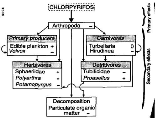
distribution-based models. These procedures, however useful, do not necessarily protect the entire ecosystem because ecological interactions are not taken into account. Apart from direct toxic effects, indirect toxic effects can occur when a reduction or elimination of susceptible species leads to a disturbance of ecological processes in the food web. These disturbances are called indirect effects and result from the direct toxic effects. To study both direct and indirect effects of the insecticide Chlorpyrifos (CPF), Brock et al. (1992a,b, 1993) applied a single dose of CPF to indoor experimental ecosystems. These mesocosms represented biotic communities from the omnipresent drainage ditches in the Netherlands. Direct effects of CPF on the drainage ditch species were studied previously (Van Wijngaarden et al. 1993) and direct effects were expected on aquatic arthropods. Fate of CPF in macrophyte-free mesocoms and its direct effects on aquatic arthropod communities has been described previously (Brock et al. 1992a). Substantial direct effects were noted on Cladocera, Copepoda, Amphipoda and some Isopoda. Indirect effects were observed on population densities of algae and invertebrates other than Arthropods (Brock et al. 1992b). The most significant indirect effect on ecosystem function was a temporary slow down of organic matter breakdown (Brock et al. 1993). A diagram illustrates the chain of events leading to indirect effects (Figure 3). Many of the indirect effects can be regarded as the result of the wipe-out of the sensitive arthropods, whereafter less sensitive organisms that were out-competed by the arthropods can increase in numbers. In order to model these competition effects, functional groups are discerned and subdivided in CPF-sensitive and inCPF-sensitive. Organisms are pooled in functional groups, by combining species with similar food preferences and with similar roles in nutrient cycling.

The aim of the model building presented in this chapter is the prediction of observed indirect effects in specific model ecosystems from the direct toxic effects, in order to validate the use of dose-response functions in CATS models.

Page 20 of 54 Report no. 719102037 ICHLORPYRIFOS:

c

I

I

-K

? ^

i

Figure 3: Direct and indirect effects of Chlorpyrifos in macrophyte-free freshwater mesocosms (+= increase, 0 = no change. - = decrease) (from Brock et al. 1993a).

3.2. Materials and methods 3.2.1. Model structure

CATS-4 (version 4.14) is a model to predict abiotic fate and effects of pesticides in

mesocosms without macrophytes. CATS-4 is built like existing CATS models (Traas et al. 1994) but incorporates a more elaborate description of phytoplankton (Janse et al. 1990, 1991, 1992). The food web is divided in the following functional groups (Figure 4): (1) Phytoplankton, subdivided in edible species for zooplankton and inedible species

due to size (consisting mainly of Volvox spec.)

(2) Zooplankton consisting of sensitive species (microcrustaceans, mainly Cladocerans and Copepods) and less sensitive Rotifera , consisting of mainly Polyarthra, Keratella spec, Synchaeta spec, Anuraeopsis spec, and Lecane spec. (Brock et al.

1992b)

(3) Molluscs feeding on algae and suspended organic matter, mainly consisting of small bivalves (Sphaeriidae) and gastropods such as Potamopyrgus Jenkinsi and Lymnea stagnalis (Brock et al. I992a,b)

(4) Shredders of deposited detritus on the sediment. Sensitive shredders are Asellus aquaticus and Gammarus pulex. An insensitive shredder is Proasellus coxalis.

Report no 719102037 Page 2Uof 54

water

C!ad.

sediment

Dipt. Turb.

Asell.

Ampli.

Proas.

•- Tubificids

Figure 4: Structure of CATS-4, with feeding fluxes and CPF processes. Other biotic fluxes (e.g. resp.) not shown. Croups susceptible to CPF are shaded.

(5) Benthic invertebrate detrivores, mainly tubificid worms, feeding on organic matter on or in the sediment. Feeding activity of tubificids is thought to be facilitated by shredding of organic matter by amphipods.

(6) Predators feeding on tubificids and zooplankton,subdivided in sensitive arthropods (mainly Chaoborus obscuripes) and less sensitive Turbellaria and carnivorous Rotifera (Asplanchna sp.).

3.2.2. Calculation of biomass of functional groups

Population dynamics in the mesocosms were monitored closely by counting the density of species per water sample water or litterbag (Brock et al. 1992a,b). However, since energy flow in CATS models is based on the law of mass conservation, biomass must be

estimated from the observed densities. For this, we made use of estimates of biomass per individual (Brock et al. pers.comm., J0rgensen et al. 1991, Van der Hoek & Verdonschot

1993). Appendix A lists the conversion factors used and the species composition of functional groups.

3.2.3. Fate of CPF

The toxicity of CPF is determined by fate and bioavailability, therefore state variables are present for both the biomass cycle and the toxicant cycle. Concentrations of CPF in water and sediment were determined by Brock et al.(1992a).

Page 22 of 54 Report no. 719102037

All biomass and detritus compartments are present as state variables in dry weight (g DW/m^) obeying the law of mass conservation. Because detritus can act as carrier for the toxicant, state variables for CPF associated with organic matter are also needed. Additional state variables are dissolved toxicant in water and pore water and are assumed to be

bioavailable. CPF sorption to organic carbon is based on equilibrium partitioning (Van der Kooij et al. 1991) and is described as a fast process. A first estimate of sorption of CPF to organic carbon (K^) is based on the octanol-water partition coefficient K^^ (Karickhoff

1981). Since the behaviour of CPF can deviate from the general pattern of hydrophobic pollutants, sorption (as determined by K^^,) is calibrated on data. The estimated K^^ is used for both suspended organic carbon and organic carbon in sediment.

Degradation of CPF in the water phase, consisting of biodegradation, hydrolysis and photolysis was described as a first-order process. Photolysis was considered small compared to hydrolysis and biodegradation (Howard 1993). Volatilization was described according to the two-layer volatilization model (US-EPA 1985). Sedimentation of

suspended matter was modelled as a net daily flux. The deposited suspended matter is assumed to be instantaneously mixed with the upper sediment layer. The highest CPF concentrations in the mesocosm sediment were found in the upper 10 mm (Brock et al.

1992a). A homogeneous upper sediment layer is assumed.

3.2.4. Modelling of direct toxic effects

Toxicity experiments with CPF on a large number of species were conducted by Van Wijngaarden et al.(l993). Their result clearly show that arthropods are susceptible species. Sometimes, several species within a sensitive functional group were tested. A choice has to be made which species should represent the sensitivity of the entire group. The function of a group of species will diminish slowly when the more sensitive species are wiped out by a toxicant. Less sensitive species are expected to keep on functioning, due to functional redundancy, untill they too are diicciQ^.Therefore, we will choose the dose-effect function of the least sensitive species per functional group to represent the sensitivity of the entire group. Toxicity data of D. longispina were regarded as representative of the sensitive group of zooplankton. Asellus aquaticus was chosen to represent sensitive shredders, and Chaeoborus obscuripes was chosen to represent sensitive carnivores. As a first

approximation, acute toxicity experiments (48 hr LC50 tests) were used for fitting of response functions, since they were available for all sensitive groups. The logistic dose-effect function was fitted to the data with SPSS software for PC using non-linear regression (Appendix B). Functional groups in CATS-4 are described as modules for algae, filter-feeders, shredders benthic detrivores and predators. The dose-effect functions were incorporated in the logistic CATS growth model (Figure 5) as described in Chapter 2. Consumed food is assimilated and the non-assimilated part is egested to become part of the detritus pools. Biomass leaves the population by respiration, predation, natural

mortality and mortality resulting from CPF toxicity. The value of dose-effect parameters determines whether or not the toxicity function is actived for a certain group.

Report no 719102037 Page 23'of 54

Egestion

"^V

Consumption

f ^

Biomass

[gDW.m -']

Assimilation

,.-Respiration

Predation

Nat. mortality

Tox. mortality

Figure 5: Generic processes of functional groups. Nat.Mortality=natural mortality.Tox. mortality mortality by direct toxicity.

3.2.5. Model implementation and calibration

The model is implemented in ACSL, a simulation language translating to FORTRAN (Mitchell & Gauthier 1993). Model calculations were performed on a 486-type personal computer. The full model consists of 12 state variables for the biomass cycle (including detritus and sediment org. matter), 6 state variables for the toxicant cycle and 2 state variables to check mass balance. CPF accumulation and effect in the mesocosms was calculated for the duration of the experiment: 10 days pre- and 119 days post CPF

application. As yet, no automated calibration with calibration routines (e.g. Aldenberg et al. 1995) has been performed.

Table 1: Specification of environmental chemistry parameters of Chlorpyrifos

Parameter

l o g K ^

fast sorption rate (/d) diffusion rale (1/d) degr. in water (/d) degr. in pore water (/d)

initial ll 3.93 0.5 0.001 0.02 0.01 calibration 2.69' 0.2 0.004 0.07 0.3

References for initial specification

(Howard 1993)

(De Nijs & Burns 1990) (Howard 1993)

(Howard 1993) Estimated from log K^^^ with regression equation by Karickhoff (1981)

Page 24 of 54 Report no. 719102037

3.3. Results

Time (days)

Figure 6: Measured and modelled (solid lines) fate of CPF in water and sediment. Data symbols: + = CPF in sediment, •* = CPF in water

3.3.1. Fate of CPF

A single dose of CPF was applied to the mesocoms, simulating unintentional

contamination of drainage ditches when applying CPF to the fields. CPF rapidly sorbs to the sediment resulting in a very fast decrease of CPF concentrations in the water phase (Figure 6). The controlling parameters for the dynamics of this process were found to be the K^^, the diffusion rate between water and sediment and degradation rates of CPF in water and sediment. Based on the log K^^ of 4.96, a high sorption to organic matter was expected. However, the use of the general equation of Karickhoff resulted in a much too high sorption to sediment. The dynamics of CPF sorption could be better reproduced by assuming a log K^^. of 2.69 and a diffusion rate between water and sediment of 0.004 per day (Table 1).

Hydrolysis, microbial degradation, and volatilizaton (in order of importance) lower the CPF concentration in the water phase further. The CPF concentration in the sediment falls rather rapidly which could not be reproduced when taking the reported degradation rates into account. It is possible that high mineralization of sediment organic matter leads to a decreasing amount of sorption sites. Such a high degradation is not likely since CPF actually inhibits breakdown of coarse organic matter (Brock et al. 1993a). Therefore, a high combined hydrolysis and microbial degradation rate was used to fit the model to the data (Table 1).

Report no 719102037 _{Page 25 of 54'} Q «-I E, Co • o

8. - i

o

I T ^1&

Time (days)

Figure 7: Simulated biomass dynamics of Cladocerans for control (+) and CPF treatment (x). Data (dotted lines): + = control, * ~ CPF treatment

Time (days)

120 Figure 8: Simulated biomass dynamics of sensitive shredders for control (+) and CPF treatment (X). Data (dotted lines): •* =CPF treatment, + =control

Page.26of 54 Report no. 719102037 CM

E

ÏT"

Time (days)

Figure 9: Simulated biomass dynamics of Dipterans for control (x) and CPF treatment ( + | Data (dotted lines): + = control, ^ = CPf treatment

3.3.2. Direct effects of CPF

The dose-effect relations for CPF on Daphnia longispina (representative of Cladocerans and Copepods), Chaoborus obscuripes (representative of sensitive predators) and Asellus aquaticus (representative of sensitive shredders) as determined in the laboratory are incorporated in the model. Very drastic effects are observed on micro crustaceans. (Figure 7). An almost complete disappearance took place after addition of CPF. Resistent life-stages of cladocerans (ephippia, Brock et al. 1992a) ensure their return when the

concentration of CPF has fallen below the acute toxic level. The general direct effects and the return of micro crustaceans after a few weeks are simulated quite adequately. The trend of decreasing micro crustacean density for both control and treated mesocosms, maybe due to ageing of the microcosms, could not yet be reproduced by the model. Direct toxicity on the sensitive shredders (Figure 8) also resulted in their disappearance from the mesocosms. Contrary to micro crustaceans, sensitive shredders did not return in the mesocosms during the time of the experiments. The model predicts the direct effect quite well but again, the dynamics of the control group are hard to match exactly with the model.

Dipteran predators are also very sensitive to CPF and they too are completely eliminated from the system (Figure 9). The simulation of the direct effects is again succesful since the Diptera are eliminated in the CPF simulation. The steady decline of Diptera in the control mesocosms to a very low level is followed by the model to a certain extent.

Report no 719102037 Page 27 of 54

- 1 0 16 4 2 OB "ST 120

Time (days)

Figure 10: Simulated biomass dynamics of algae for control (x) and CPF treatment (+). Data (dotted lines): + = control, ^ = CPF treatment

3.3.3. Indirect effects

Algae were initially subdivided in small edible algae and large inedible algae, mainly Volvox. Due to difficulties with phytoplankton dynamics, Volvox is temporarily excluded from the food web and total algae are simulated. The simulation of the algal biomass in the control mesocosms is higher than observed (Figure 10). The CPF treatment results in higher biomass peaks in the mesocosms because grazing by micro crustaceans is

eliminated by CPF. The model response is about 3 to 4 times stronger than observed in the cosms, but does show the stimulatory effect resulting from direct toxicity on micro crustaceans.

Due to the release of competition by direct toxicity on micro crustaceans, Rotifera biomass increases sharply in the CPF treated cosms compared to the controls (Figure 11). The simulation of this indirect effect is less dramatic but correct. The indirect, stimulating effect on Rotifera continues far longer than observed in the mesocosms. On comparison of Figures 7 and 11, it is obvious that Rotifera decline again when the direct toxicity on Cladocera and Copepoda is no longer present and micro crustaceans regain their previous density.

In the mesocosms, the sudden increase of Rotifera after CPF addition is controlled by an increase in carnivorous Rotifera, mainly Asplanchna (data not shown). In the present model, Rotifera are kept in check by the insensitive predators, including predaceous Rotifers, but the model response of the predators to the increase of Rotifera cannot match the observed behaviour of carnivorous Rotifera.

Page 28 of 54 Report no. 719102037 O o>

E,

S

o

Time (days)

Figure 11: Simulated biomass dynamics of Rotifera for control (x) and CPF treatment (•¥). Data (dotted lines): + = control, •* = CPF treatment

120

Time (days)

Figure 12: Simulated biomass dynamics of insensitive shredders for control (+) and CPF treatment (x). Data (dotted lines): + = control, -* = CPF treatment

Report no 719102037 Page 29 of 54

120

Time (days)

Figure 13: Total organic matter in sediment without CPF ( marked x) and as a indirect effect ( tnarked +) of CPF addition (only simulations shown).

Decomposition of organic matter in litter bags was inhibited in the first four weeks after CPF. addition. This was ascribed to a decrease in sensitive shredders (Asellus and

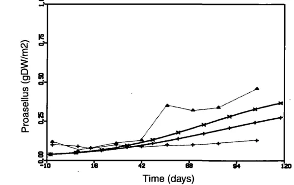
Gammarus) and by a decrease in oligochaete worms (Brock et al. 1993a). This decrease could be counter acted by a small increase of insensitive shredders, mainly Proasellus coxalis (Figure 12). The model could reproduce the behaviour of this group, albeit with slightiy different dynamics. Simulation results showed an overall temporary inhibition of organic matter breakdown in the sediment (Figure 13). After day 84, the decrease

continues with apparentiy the same rate as before. Since the sensitive shredders do not return in the simulation, the cause for the transient inhibition in the model can be at least partly different from the explanation offered by Brock et al.

3.4. Discussion 3.4.1. Fate of CPF

During calibration it became clear that the partitioning of CPF is determined by sorption to organic matter, the diffusion rate from water to sediment and the degradation rate of CPF in water and sediment. CPF was assumed to be instanteneously mixed in the model, but in reality, the partitioning of CPF over the water column and sediment depth is not homogeneous. The simplification used in the model proved to be justified since the gradient of concentrations in the water column disappeared within a day. For sensitive

Page 30 of 54 ,- Report no. 719102037 arthropods, effect concentrations were exceeded everywhere in the water column, within a few hours after application of CPF. Stratification in mesocosms with macrophytes (mainly Elodea nuttallii) proved to be more persistent (Brock et al. 1992a) and resulted in higher survival of sensitive arthropods. Stratification is probably more important when modelling Elodea-domimted mesocosms.

3.4.2. Direct effects

Direct effects of CPF are determined by the exposure concentration in the water column, with probably negligible contributions from- the sediment. The dynamics of the direct effects on arthropods proved to be highly correlated with the concentrations in the water column. However, only the parameters for abiotic fate had to be calibrated. The

parameters for direct toxicity based on laboratory toxicity testing did not have to be changed in any way The conclusion of Brock et al. (1992a) that exposure uncertainty is often larger than effect uncertainty seems to be confirmed by our calibration of both fate and direct effects.

Direct effects in this experiment are predicted very well with the dose-response relation of a 'key species' within a functional group. Based on a priori knowledge of the mode of action of CPF, a correct subdivision could be made of sensitive and insensitive species. When we have less a knowlegde of the mode of action of a toxicant, and sensitivities of species are widely different, it may be much more difficult to sensibly subdivide the ecosystem.

3.4.3. Indirect effects

Major indirect effects are expected on direct producers since grazing pressure of Cladocera and Copepoda is at least temporarily relieved. Since we only have one group of

phytoplankton in our model, competition effects between small inedible and large edible algae could not be simulated. The increase of average phytoplankton in the simulation is in agreement with data but much larger than observed. Due to the release from

competition, Rotifera and Sphaeridae profit according to Brock et al. (1992a,b) but only Rotifera does so to a limited extent in the simulation. It can be concluded that the interplay between phytoplankton and herbivores is a subtle one which the present model approximates but more work needs to be done.

Indirect effects on shredders and detrivores were not simulated easily. As a first assumption, all organic matter in the sediment was presumed available as food for the shredders. More realistic dynamics resulted when we assumed only fresh detritus to be available as a limiting resource for competition between shredders.

The decline of Oligochaetes was attributed to increased predation by Turbellaria and Hirudinea (Brock et al 1992b, 1993a). The availability of food for detrivores such as Oligochaete worms could be related to the total processing capacity of shredder groups. In this way, a decline in shredder activity by direct toxicity would also lead to a lower Oligochaete density.

Report no 719102037 Page 31 of 54

Hirudinea and Turbellaria form the group of insensitive carnivores. Therefore, competition between them could not be taken into account, although the results of the mesocosm studies indicated that competition may occur. The differences in prey composition between these types of predators are not known very well which exemplifies the problems of

analyzing the structure of ecosystems during model formulation. The less defined the ecological niche of species, the more problems arise with the allocation to functional groups.

This study has shown that a thorough knowledge of ecosystem structure and trophic relationships as collected in the mesocosm experiments is essential for succesful

simulation of direct and indirect effects. What this study has also shown is that ecological effect modelling requires an integration of mechanisms for fate and direct toxicity and ecological knowlegde of the system at study. The present model is an example that ecosystem complexity can be reduced to the level of functional groups in order to study and partly explain the ecological mechanism leading to secondary effects.

Report no 719102037 Page 33-of 54

4. CALCULATING HAZARDOUS CONCENTRATIONS FOR ECOSYSTEMS BY MEANS OF THE CATS-2 MODEL

4.1 Introduction

In Chapter 2, a method was presented to integrate dose-response relationships from laboratory toxicity testing in food web models. This provides a tool to predict direct and indirect effects of toxicants in food webs. In chapter 3, the effects of Chlorpyrifos in a mesocosm experiment were modelled with the CATS-4 model. The results made clear that direct toxicity as observed in the mesocosms could be modelled quite adequately. Indirect effects on the level of functional groups, as predicted by the CATS-4 effect model, showed good general agreement with the nature of the observed indirect effects. The main goal of this chapter is to use CATS effect models for an ecological

underpinning of environmental quality objectives. In mesocosm experiments, populations are defined as affected if species numbers show a significant increase or decrease

compared to the control situation (Brock et al. 1993b). Recovery of affected ecosystems is defined as a return to the normal range of numbers in the control systems. In CATS

models, species numbers are converted to total biomass per functional group. Toxic effects are therefore expressed as deviations from control biomass, as shown in chapter 3. Since both direct and indirect effects may occur, the biomass deviations can be either positive or negative and they may occur anywhere in the food web.

We define the Hazardous Concentration for the Ecosystem (HCE) as the concentration where the food web is disturbed to an extent that we find unacceptable. We tentatively propose to regard a 5 % deviation of control biomass, no matter where it occurs in the food web, as the HCE for a particular toxicant (Figure 14). Because substantial

uncertainty exists in model parameters, the HCE is calculated in the framework of Monte-Carlo analysis (Traas & Aldenberg 1994). Hereto, a number of dose-response relationships for relevant organisms has been embedded in existing CATS models. HCEs were

calculated for Cadmium, Tributyltin (TBT), a fabric softener ditallow dimethyl ammonium chloride (DTDMAC) and the insecticide Chlorpyrifos (CPF). Since control biomass has associated uncertainty, the 5% deviation of control biomass is calculated for each single Monte Carlo run and leads to probability distributions for the HCE.

4.2 Materials and Methods 4.2.1 Dose-effect modelling

Toxicity experiments performed in the laboratory were used to fit the logistic dose-effect function to the data with SPSS® software (chapter 2), using non-linear regression. Species

Page 34 of 54 ' Report no. 719102037

are used that are ecologically relevant (Table 2). It was not possible to find dose-effect relations for all functional groups in the model. Relations found are integrated in the CATS model as described in chapter 2. The model that is used for all calculations is CATS-2 for lakes without macrophytes. Some of the species used for dose-effect

modelling are not present in the lake ecosystem but related species are. This is far from ideal, but is due to the lack of full data sets that can be used for dose-effect modelling. For the same reason, no food-chain bioaccumulation is taken into account.

4.2.2 Fate modelling

For each toxicant, fate and abiotic cycling was modelled. Parameters determining the fate are sorption to suspended matter and sediment, volatilization, degradation in water and sediment, uptake by organisms (Appendix C). Uptake of Cd and TBT has been calibrated previously (Traas et al. 1994,Traas et al. 1995). Uptake of CPF and DTDMAC by

organisms could not be studied in detail. 4.2.3 Calculation of HCEs

In laboratory toxicity tests, animals are exposed to the test solution and uptake from water takes place by filtering, ventilation over gills or dermal passage. It is assumed that the exposure concentration as given in the toxicity experiments are bio-available

concentrations. In CATS models, the toxicant is allowed equilibrium partitioning of the toxicant between water, suspended matter and sediment. The calculated dissolved

concentration in the water phase of the model is considered to be the exposure concentration as in the toxicity tests.

Essential to the calculation of HCEs is the deviation from the control biomass as a result of toxic effects. The normal range of biomass of a certain population can be quite wide (Vanhemelrijk 1993). CATS models are calibrated on normal ranges of biomass by means of a Monte-Carlo procedure (Traas & Aldenberg 1994). Each model run consists of new parameter combinations, leading to new estimates of biomass, that are tested against the normal ranges of biomass. Succesful parameter combinations lead to biomasses in the foodweb that conform to the normal ranges of the ecosystem, and are used for HCE calculations. The dose-response functions are mainly determined in acute toxicity tests. Since the duration of the toxicity test is taken into account (Chapter 2, eq. 6-7), correction is applied for the short duration of most toxicity tests. However, no comparison of the estimated mortality rate has as yet taken place between dose-response relations derived from acute and chronic tests. The outcome of the HCE calculations thus depends on the type and number of dose-response functions that are incorporated in the model.

In summary, the calculation of the HCE consists of the following steps:

- Generation of parameter combinations by Monte-Carlo sampling (Traas et al. 1994) - Model calculations until the biomass reaches steady-state. This is the control biomass

Report no 719102037 Page 35 of 54

Comparison of steadystate with normal ranges as part of the calibration procedure. -If the run is accepted, the concentration is increased from zero with small steps, and the resulting biomass is compared with the control biomass every step. If biomass of some group deviates more than 5% from the control biomass, no matter where in the food web, the run is stopped and the HCE is stored on disk for the concentrations in the water phase, water including suspended matter and sediment. The functional group that is responsible for the 5% deviation is recorded, as this may vary depending on the parameter values.

- This procedure is repeated until several hundreds of runs are performed

- After completion of the Monte-Carlo runs, the distribution of HCEs, as written to disk, is used to calculate basic statistics with SPSS.

E D 0) to to E to to CO E o 2 ) _.25 3 Br ivin g duck s i .7 5 1 biomas s d .0 0 0 o ^ • -üü;

r

'1

J

N

s

cadmium dissolved (fig/l)

Figure 14: Direct toxicity ofCd on Bivalves (Kraak et al. 1992) and indirect effects on ducks. The HCE is reached when the 5% deviation lines (dotted) are crossed.

4.3 Results

4.3.1 Fitting dose-response functions

Raw data from acute toxicity tests were collected for fitting logistic dose-response functions. Data availability is poor since usually, only LC50's, EC50's or NOECs are reported without specification of the underlying function. Most data used were made available by RIVM and SC-DLO. For cadmium and CPF, no problems were encountered with non-linear regression. The functions for DTDMAC on zooplankton and TBT on

Page 36 of 54 Report no. 719102037

Chlorella were estimated from reported NOEC and LC50s.

Table 1 Overview of dose-response functions from laboratory toxicity testing for 4 toxicants

toxicant cadmium CPF TBT DTDMAC Cadmium species Daphnia magna^ Casterosteus aculeatus^ Simocephalus vetulus** Aseltus aquaticus'' Gasterosteus aculeatus** Daphnia magna^ Gasterosteus aculeatus*^ Chlorella pyrenoidosa ^^ ^^ '^ Daphnia magna^ Chironomus riparius'' Gasterosteus aculeatus'' Dreissena polymorpha ^ a (LC50) 0.15 12.67 0.45 2.55 9.49 1.70 13.41 42.61 2.04 6.55 5.21

f

Data from RIVM-ECO (Roghair et al.), experiment 91/P049, mortality

Data from (Kraak et al. 1992), longest exposure time used, see eq. 9, chapter 2, filtration Data from RIVM-ECO (Roghair et al.) experiment 89/P041,mortality

Data provided by SC-DLO, from experiments (Van Wijngaarden et al. 1993), mortality Data from (Matthijsen Spiekman et al. 1989), growth

Data from (Roghair 1984), mortality

Estimated from (Overleggroep deskundigen wasmiddelen milieu 1988), mortality Data from (Roghair et al. 1992), mortality

Report no 719102037 " " Page 37 of 54

Table 2 Frequency of direct (marked *) and indirect effects for all functional groups in the food web model for different HCE calculations.

phytopl. zoopl. chironomids benthic detrivores bivalves omn. fish pred. fish benth. fish diving ducks fish-eating birds Cd 37.6 %' 40.4 %' 0.0% • 4 . 9 % 0.5 % 16.6% CPF 91.2 %' 0.0% * 0.0%' 7.5% 0 . 5 % 0 . 8 % TBT 1.5 %' 92.0 %' 0.0% * 5.7% 0.5 % 0.3 % DTDMAC 84.1%* 6.0% 0.0%* 8.6% 0.5 % 0 . 9 %

4.3.2 Direct and indirect effects.

Direct toxic effects are expected to play an important part in the determination of the HCE. Because of parameter variation, each Monte Carlo run may lead to a different HCE concentration with a different functional group responsible for the HCE. Table 3

summarizes the frequencies with which functional groups are responsible for the HCE. Zooplankton generally is a sensitive group, in consequence direct effects on zooplankton determine the HCE for CPF, TBT and DTDMAC to a great extent. Filtration of

Dreissena polymorpha is very sensitive to heavy metals (Kraak et al. 1992, 1994) and direct effects of cadmium are responsible for the HCE in 40.4 % of cases.

The frequency of indirect effects varied between 6.5 and 22 %. Due to the direct effects on bivalves, the diving ducks reach the critical biomass deviation first in 16.6 % of all Monte-Carlo runs. Indirect effects on fish are noted for all toxicants, but with much lower frequencies. All observed indirect effects are negative biomass deviations (results not shown). Positive biomass deviations, by release from competition as observed in chapter 3. have not been noted in this case. The species most responsible for the HCE is usually the most sensitive species. Some direct effects on fish are never responsible for the HCE (0.0%), indicating that direct toxicity on these species occurs at concentrations above the calculated HCE.

Page 38 of 54 Report no. 719102037 4.3.3 HCE calculations

Uncertainty in model parameters for the fate of the toxicants but also for the food web leads to different HCE concentrations with each parameter combination. HCE distributions for the different abiotic compartments are plotted as boxplots in Figures 15 to 17. Note the different units for the fabric softener DTDMac.

The lowest HCE is reached for cadmium if we consider the dissolved concentration (Fig. 15), ranging between 0.01 and 0.13 pg/l. The HCE concentration range of CPF is a littie higher at 0.1 to 0.28 pg/l. TBT appears to be less toxic with a range of 0.04 to 1.6 pg/l. Toxicity data for mollusca, which are most sensitive toTBT, could not be included for lack of an appropriate dose-response function.

DTDMac is the least toxic compounds since its toxicity is in the mg/l range.

The HCE based on available cadmium is lower than for CPF, while the HCE based on total water concentrations is lower for CPF than for Cd (Figure 16). This illustrates that toxicity of the compounds is not determined from exposure to suspended matter, on the contrary, sorption of the toxicant to suspended matter decreases toxicity by making the toxicant unavailable for direct exposure.

Cadmium in sediment is in the range of 10 to 50 mg/kg dry sediment (Figure 17). For CPF, allowed sediment concentrations are much lower and range between 0.001 and 3.1 mg/kg. TBT occupies an intermediate position with a range between 0.02 cuid 6.8 mg/kg. Again, much higher concentrations are found for DTDMac in water ranging between 0.1 and 8.3 mg/kg.

1 .5

•1 .0

Report no 719102037 Page 39 of 54

2 .5 H

Cd

CPF

TBT

DTDMac

Figure 16: Box plots for total water concentrations (incl. suspended matter) of the HCE for 4 toxicants.

5 0

E

E

3 0

2 0

1 0

g/kg

1 1

0 ^ - - n ^ ^ — I r

Cd CPF TBT DTDMac

Page 40 of 54 Report no. 719102037

4.3.4 Comparison of HCEs with environmental quality objectives

HCE calculations are summarized (Table 4) and compared to different environmental quality objectives to illustrate the order of magnitude of HCEs. Existing quality objectives are usually based on extrapolation of laboratory-derived NOECs (VROM 1994, van de Plassche 1994). HCEs are based on 5% loss of total functional group biomass. The

uncertainty in the determination of the HCE will be considered in the comparison. To stay on the safe side of the HCE distribution, the 5th or the 25th percentile could be chosen for comparison. To allow interpretation of the HCE distributions (Figures 15-17), the fifth and the 25th percentile and the median are shown in Table 4.

For cadmium and TBT, a comparison was made between HCEs and the Target and Limit Values as used by the Ministry of Housing, Spatial Planning and the Environment. The 5th and 25th percentile of cadmium HCEs are in the same order of magnitude as existing Limit Values. A recentiy proposed limit of 0.35 ug/1 (van de Plassche 1994) is however higher that the HCEs calculated here. The HCE calculated for sediment is in the same range as the maximum permissible sediment concentration of 29 mg/kg proposed by Van de Plassche (1994).

HCEs calculated for TBT in water are more than two orders of magnitude larger than the present Limit Values. This is probably due to the lack of dose-response relations for molluscs, who are known to be very sensitive to TBT. The HCE for sediment (based on equilibrium partitioning) is much higher than the Limit Value. In general, the width of the distributions is small as judged from a comparison of the 5th percentile and the median. This is due to the use of selected parameter combinations from a calibrated model for Lake Westeinder (Traas et al. 1995).

CPF is an insecticide that is also quite toxic to crustaceans and fish. The 5th percentile of the HCE for water is in the same range as proposed by Van de Plassche, and the same holds true for sediment.

DTDMac has the highest proposed Limit-Target Values of the 4 toxicants. The range of DTDMac HCEs is quite wide since much uncertainty still exists regarding its sorption behaviour (Appendix B). The median of the DTDMac distribution for water is one order of magnitude higher than the proposed Limit Values as estimated from a set of NOECs (Roghair et al. 1992, Van Leeuwen et al. 1992).

Report no 719102037 Page 41 of 54

Table 3 Con^arison of calculated Hazardous Concentrations for Ecosystems with environmental quality objectives (n.a. = not available, n.d. = not determined).

Toxicant Cd CPF TBT DTDMac Compartment water (ug/l) total water (ug/l) sediment(mg/kg) water(ug/l) total water (ug/l) sediment(mg/kg) water(ug/l) total water (ug/l) sediment(mg/kg) water(ug/l) total water(ug/l) sediment(mg/kg) 5th Perc. 0.031 0.29 7.3 0.008 0.01 0.002 1.35 1.52 0.08 n.d. n.d. n.d. 25th perc. 0.11 0.83 22.5 0.23 0.28 0.10 1.36 1.53 0.96 395 489 331 Median 0.12 1.06 27.6 0.25 0.31 0.35 1.42 1.61 2.31 446 573 1289 Target Value 0.01" 0.05= 0.8" 2.8E-5'' n.a. 1.1 E-5'' 0.000 r 0.000 r 0.0001= 0.5^ n.a. n.a. Limit Value 0.06" 0.2' 2.0" 0.0028'' n.a. 0.0011"

o.or

o.or

" Target Values and Limit values are Dutch environmental quality objectives (VROM 1994). '' Proposed Limit Value (MPC) and Target Value (NC) taken from van de Plassche (1994) ^ Proposed in DTDMac studies (Roghair et al. 1992, van Leeuwen et al. 1992).

Page 42 of 54 Report no. 719102037

4.4 Discussion Data availabilitv

Extrapolation procedures used for the derivation of quality objectives are usually hampered by limited availability of data (van de Plassche 1994) and this study is no exception. A short survey of available literature suggested that the availability of raw chronic LC50 or EC50 data is probably even worse. In this particular study, we used data collected at our institutes for all toxicants studied. Three dose-response functions for three different functional groups were incorporated in the model, usually two invertebrate and one fish group. It proved impossible to find data for all groups in the model. Groups always consist of many species and therefore it would be nice if the distribution of species sensitivities within a group was known. For CPF it was possible to choose the representative dose-response relationship from the observed dose-response in the mesocosms. For the other

compounds, no such choice could be made since only one dose-response relationship was available per functional group. As in any extrapolation method, the outcome of HCE calculations depends on the species tested and the number of species used.

In the present study, indirect effects result from direct toxicity. Transfer of toxicants through the foodchain can also be considered an indirect effect. This aspect was not taken into consideration in this study, but only due to a lack of dose-response studies with relevant predators. Food chain-transfer of cadmium and TBT has been modelled before (Traas et al. 1994, 1995), but data for food chain transfer of CPF and DTDMac are missing.

Nature of predicted indirect effects

In chapter 3, positive biomass deviations were observed due to resource competition. This could be simulated by making a distinction between sensitive and insensitive species within a functional group. Which species belonged to which subgroup was quite clear a posteriori because of the extensive knowlegde of the mode of action of CPF and

laboratory toxicity testing (Van Wijngaarden et al. 1993).

In CATS-2 no distinction could be made between sensitive and insensitive species within a functional group. This is partly due to lack of toxicity data, but maybe even more so to a lack of ecological specificity. The model from chapter 3 was used in a well defined experimental setup. A more generic model structure was used for calculating HCEs in chapter 4. In that case, toxic effects will lead to less growth or a higher mortality for the entire functional group, since no internal subdivision between sensitive and insensitive was made.

Given these reservations, indirect effects were predicted for all toxicants, especially so for cadmium. Unintentional effects on non-target organisms do occur, but with a low frequency. The exact nature and extent of these indirect effects are more tentative than

Report no 719102037 Page 43 of 54 those from chapter three. It seems that indirect effects are not very sensitive since the direct toxicity always occurs with the highest frequency. This may not come as a surprise, since direct effects always precede the indirect effects. Even if this occurs with a low frequency, it is serious enough to consider when deriving quality objectives.

Species sensitivity

In chapter 3, we used the dose-response function of the least sensitive species to represent the entire functional group.The rationale behind this is that the group as a whole is not wiped out when toxicity occurs on the most sensitive organisms, due to functional redundancy. The functioning of the group is seriously damaged if the less sensitive organisms are affected. For the other compounds, there was no choice to make. The ecological role of organisms that are susceptible determines the type and extent of the indirect effects of a toxicant. The specific elimination of micro crustaceans in chapter 3 led to an increase in algae that were kept at a low biomass by grazing pressure. After release from competition, Rotifera increased sharply but shortly. Rotifera could not take over the role of the Cladocerans maybe because of a lower filtration rate and increased predation. The a priori knowledge of the toxicant CPF leads to meaningful calibration of the sensitive Cladocerans and insensitive Rotifera. Therefore, an adequate representation of the observed indirect response can be made. The subdivision of species into a sensitive and insensitive group becomes trivial without knowledge of the target organisms and the ecological properties of such groups. More insight in the distribution of species sensitivity within functional groups is esssential for adequate ecological dose-response modelling. Experiments such as the ones used for chapter 3 can provide the basis for ecologically sound use of observed dose-response functions in ecosystem models.

HCE calculations

The previous sections have shown that many uncertainties still exist in the calculation of ecosystem response to toxicants. Model uncertainty is mainly determined by biological variation within functional groups, fate of the chemical (Traas et al. 1995) and uncertainty about dose-response relations (Aldenberg 1995). Uncertainty in dose-response relations has not been addressed in the present calculations yet, nor the uncertainty in functional

response of functional groups due to sensitivity variation within the group. Additionally, some corrrection may be necessary in the extrapolation from acute to chronic exposure, even though time of exposure is a model parameter.The presented HCE distributions should therefore be regarded as a first estimation of our uncertainty regarding ecosystem effects. Since the HCE criterion is set at 5% mortality of an entire functional group and not just exceedance of an NOEC, evaluation of the HCE should be on the safe side. Therefore, it seems appropriate to look at the median HCE but also low percentiles of the HCE distributions, e.g. the 5th or 25th.

Page 44 of 54 • Report no. 719102037

It is surprising to find that even with only three dose-response functions for mortality per toxicant, the left tail of the HCE distributions is often close to (proposed) Limit Values. The exception is DTDMac and TBT, where almost all of the HCE distribution is higher than the proposed Limit Values. Since all calculated HCEs are higher than (proposed) Limit Values, Limit Values provide enough protection, at the chosen 5% level of mortality for some functional groups.

We could state that ecosystem effects occur at higher concentrations than existing quality standards, and be reassured that quality standards are adequate. It can also be concluded that the function of the ecosystem is disturbed leading to 5% biomass devations of entire functional groups, predicted with only a few dose-response functions, at concentrations relatively close, but higher than existing Limit Values. Given the fact that only a few possible dose-response functions are incorporated in the HCE calculations, it can be expected that HCEs can get close to Limit Values with a more elaborate data set. HCE calculations depend strongly on the fate and bio-availability of the toxicant. Differences in ecosystem structure, such as the presence of aquatic macrophytes, can influence fate and thereby ecological effects considerably, leading to different HCEs for different ecosystem structures. More insight in these modulating factors is urgently needed. Given the

limitations of HCE calculations, it seems that ecological effects of toxicants can be expected at concentrations higher, but relatively close to (proposed) Limit Values.

An interesting comparison could be made between a HC5 (Aldenberg & Slob 1993) and HCE calculations for different ecosystems. To allow this, the same data should be used for estimating both the NOECs (for HC5 calculations) and dose-response functions (for HCE calculations). This CPF data set presented in chapter 3 seems adequate for such a study. It would then be possible to indicate which percentage biomass deviation used for the HCE calculations leads to comparable quality standards as the HC5 and ascertain whether ecological disturbance takes place at the calculated HC5, or at higher concentrations as the present HCE calculations suggest.

Report no 719102037 Page 45 of 54^

5. CONCLUSIONS

Dose-response functions can be fitted on data from laboratory toxicity tests and were used to predict the response of functional groups in food webs. No special requirements are necessary to increase the information value of LC50 tests, except that the raw data from LC50 tests are made available.

Primary effects of CPF in a food web, as observed in mesocosm experiments, could be modelled adequately by incorporating dose-response functions in a CATS model. Indirect effects of CPF on functional groups in a food web, resulting from direct toxicity, could be modelled by allowing competition for food within functional groups. The nature of the indirect effects could be predicted.

The ecosystem response to toxicants was used to propose a quality standard called the Hazardous Concentration for Ecosystems (HCE). Both direct and indirect effects detemiine the HCE.

Based on model simulations, the HCE is mainly determined by the direct effects but indirect toxic effects can also determine ecosystem damage before direct toxicity becomes apparent.

The outcome of HCE calculations depends, like any other extrapolation technique, on the number and sensitivity of species used for the calculations. The advantage of HCE calculations is that they can be performed for specific ecosystems and locations. The calculated HCEs for cadmium, Chlorpyrifos and DTDMAC are higher, but within two orders of magnitude of (proposed) Limit Values. Ecological effects of cadmium and CPF, defined as a 5% deviation from control biomass, could occur at concentrations close to ( proposed) Limit Values.