Health survey on people living in the direct vicinity of agricultural plots: additional analyses | RIVM

Health survey on people living in

the direct vicinity of agricultural

plots: additional analyses

RIVM report 2020-0056

M. Simões et al.

additional analyses

Colophon

Parts of this publication may be reproduced, provided acknowledgement is given to the: National Institute for Public Health and the Environment, and the title and year of publication are cited.

DOI 10.21945/RIVM-2020-0056 M. Simões (author), Utrecht University A. Huss (author), Utrecht University L. Portengen (author), Utrecht University R. Vermeulen (author), Utrecht University C. Baliatsas (author), Nivel

M. Dückers (author), Nivel R. Verheij (author), Nivel N. Janssen (author), RIVM K. Rijs (author), RIVM J.P Zock (author), RIVM Contact:

Jan-Paul Zock

Centre for Sustainability, Environment and Health jan-paul.zock@rivm.nl

This investigation was performed by order, and for the account, of the Ministry of Health, within the crop protection product policy framework

Published by:

National Institute for Public Health and the Environment, RIVM

P.O. Box1 | 3720 BA Bilthoven The Netherlands

Synopsis

Health survey on people living in the direct vicinity of agricultural plots: additional analyses

Generally speaking, persons living within 250 metres of agricultural plots where pesticides are used do not have more health problems than persons with few or no agricultural plots in the vicinity. This conclusion is in agreement with the results of an exploratory study from 2018, which was based on different points of departure.

There are a few exceptions of this general pattern from the two analytical approaches. Living near maize plots coincided with a higher risk of death due to chronic lower respiratory diseases. Furthermore, leukaemia death possibly occurred more often near rotating crops (grain, beets, potatoes) and suicide seemed to occur more often near plots where grains are cultivated. With the available information it was not possible to explain these findings.

More specific research is needed to learn more about the relationship between pesticides and the health of persons living nearby. The researchers recommend obtaining better estimates of the exposure to specific pesticides. In addition, such research must focus on COPD and other health problems that are regularly mentioned in the scientific literature, such as leukaemia, Parkinson’s disease and cognitive effects. More information is also needed on individual factors that have an effect on health, such as lifestyle.

This is made clear by research carried out by RIVM, Utrecht University, and the Netherlands Institute for Health Services Research (Nivel). The research discussed here supplements research carried out in 2018 into the health of persons living in the direct vicinity of agricultural plots of specific crops. The Health Council of the Netherlands will advise the government on which follow-up research should be carried out. The Ministry of Health, Welfare and Sport requested these additional analyses. This request was motivated by research carried out in 2019, coordinated by RIVM, into the exposure to chemical pesticides of persons living in the direct vicinity of bulb fields. This research

concluded that the concentrations of pesticides in household dust within 250 metres of the bulb fields treated with pesticides did not show much difference. The differences were greater with regard to houses located at a distance of more than 500 metres from the bulb fields.

Keywords: agriculture, pesticides, exposure, health survey, people living in the vicinity, land use, re-analysis

Publiekssamenvatting

Gezondheidsverkenning omwonenden van landbouwpercelen: Aanvullende analyses

Mensen die binnen 250 meter van landbouwpercelen wonen waar bestrijdingsmiddelen worden gebruikt, hebben over het algemeen niet méér gezondheidsproblemen dan mensen met geen of weinig

landbouwpercelen in de buurt. Deze conclusie komt overeen met de resultaten van een verkenning uit 2018. Hierin waren andere

uitgangspunten gebruikt.

Er zijn een paar uitzonderingen op dit algemene beeld uit de twee

verkenningen. Het wonen dicht bij maisteelt lijkt samen te gaan met een grotere kans op overlijden aan luchtwegaandoeningen. Verder is dicht bij roulatieteelt granen/bieten/aardappelen mogelijk meer sterfte door leukemie en lijkt dicht bij graanteelt meer zelfdoding voor te komen. Met de beschikbare gegevens was het niet mogelijk om deze bevindingen te verklaren.

Specifieker onderzoek is nodig om meer te weten te komen over de relatie tussen bestrijdingsmiddelen en de gezondheid van omwonenden. Als daartoe wordt overgegaan dan adviseren de onderzoekers om de blootstelling aan specifieke bestrijdingsmiddelen gedetailleerd in kaart te brengen. Centraal in dat onderzoek zouden dan kunnen staan COPD en andere gezondheidsproblemen die in de wetenschappelijke literatuur regelmatig naar voren komen, zoals leukemie, de ziekte van Parkinson en cognitieve effecten. Daarvoor is dan ook meer informatie nodig over individuele factoren die invloed hebben op de gezondheid, zoals leefstijl. Dit blijkt uit onderzoek van het RIVM, de Universiteit Utrecht en het Nivel. Het onderzoek is een aanvulling op onderzoek uit 2018 naar de gezondheid van omwonenden van landbouwpercelen voor bepaalde gewassen. De Gezondheidsraad gaat het kabinet adviseren welk vervolgonderzoek moet worden uitgevoerd.

VWS heeft om deze aanvullende analyses gevraagd. Aanleiding was onderzoek uit 2019, gecoördineerd door het RIVM, naar de blootstelling van omwonenden van bloembollenvelden aan chemische

bestrijdingsmiddelen. Daaruit bleek dat de concentraties

bestrijdingsmiddelen in huisstof binnen 250 meter tot de bespoten bloembollenvelden weinig verschilden. Er waren meer verschillen ten opzichte van woningen op meer dan 500 meter van de bloembollenvelden. Kernwoorden: landbouw, bestrijdingsmiddelen, gezondheidsverkenning, omwonenden, landgebruik, heranalyse

Contents

Samenvatting — 9

1 Introduction — 13

2 Methods — 15

2.1 Screening analysis - exploring the nature of the exposure - outcome

associations — 15

2.2 Correction for multiple testing — 17

2.3 Main analysis – models A, B, C and D — 17

2.4 Further analyses — 18

2.4.1 Covariates (confounders and effect modifiers) — 18

2.4.2 Sensitivity analyses — 18

2.4.3 Stratified analysis by region — 18

2.5 Interpretation criteria — 19

2.5.1 Q-value (adjusted p-value) < 0.10 — 19

2.5.2 Statistically significant effect on the ‘high exposure group’ — 19

2.5.3 Robust estimate after sensitivity analyses and after comparing with a

minimally adjusted model — 19

2.5.4 Low heterogeneity — 20

2.5.5 Remark on the interpretation — 20

2.6 Other exposure metrics — 20

2.7 Specific methods for the data sets used — 20

2.7.1 General model framework — 20

2.7.2 Sensitivity analyses — 22

2.7.3 Model without confounders and stratified analysis — 22

2.7.4 Interpretation — 23

2.8 Re-analysis of mortality outcomes — 26

3 Results — 27

3.1 Total and cause-specific mortality — 27

3.1.1 Association between grains and suicide mortality — 30

3.1.2 Re-analysis using the original method — 30

3.2 Health Monitor outcomes — 30

3.3 Perinatal outcomes — 31

3.4 Nivel Electronic Health Records from GP registries — 31

3.5 Nivel questionnaire survey — 31

4 Discussion — 33

5 References — 35

6 Appendices — 37

Appendix 1 Overview of the models (0, A, B, C or D) that best explained the association between the explored outcomes exposure (crop) pair — 38

Appendix 3 Glossary. Standardised terminology in English and Dutch for crops and health endpoints — 49

Samenvatting

In juli 2018 is een onderzoek gepubliceerd naar gezondheidsproblemen van omwonenden van landbouwpercelen waar bestrijdingsmiddelen worden gebruikt. In deze zogenoemde gezondheidsverkenning is onderzocht of de gezondheid van omwonenden samenhangt met de nabijheid van specifieke gewassen. Hierbij is gekeken naar oppervlakte van de percelen op verschillende afstanden (<50, 50-100, 100-250 en 250-500 meter) van het woonadres.

Naar aanleiding van de publicatie in april 2019 van de resultaten van een parallel onderzoek naar de daadwerkelijke blootstelling aan chemische bestrijdingsmiddelen van omwonenden van

bloembollenvelden, heeft het Ministerie van VWS het RIVM gevraagd om aanvullende analyses naar de relatie met gezondheidsproblemen uit voeren. Uit het blootstellingsonderzoek bleek namelijk dat de

concentraties bestrijdingsmiddelen in huisstof binnen 250 meter van een bespoten bloembollenveld relatief weinig van elkaar verschilden. Het verschil in blootstelling was groter en duidelijker als de concentraties van woningen binnen 250 meter werden vergeleken met die van woningen op tenminste 500 meter afstand van het bloembollenveld. Dit riep de vraag op of de gebruikte afstandsmaten in de

gezondheidsverkenning wel voldoende onderscheidend waren om verschillen in gezondheid tussen verschillende afstanden binnen 250 meter te kunnen aantonen. Omdat dit een criterium was voor het identificeren van associaties met gezondheid, zouden we mogelijk relevante verbanden hebben gemist. Voorliggende rapportage beschrijft derhalve de resultaten van aanvullende analyses naar de relatie tussen het wonen binnen 250 meter van landbouwpercelen en

gezondheidsproblemen. Hierbij is de aanname vervallen dat er een trend zou zijn van meer gezondheidsproblemen bij een kleinere afstand (<50m, 50–150m, 150-250m) tussen het landbouwperceel en de woning.

Voor de deelanalyses van sterfte en doodsoorzaken konden we door voortschrijdend inzicht een gegevensbestand met méér mensen gebruiken dat nog steeds aan de oorspronkelijke criteria voldeed. We hebben ter controle voor sterfte en doodsoorzaken ook nog de methode uit het vorige rapport toegepast op dit geactualiseerde, grotere bestand. Methoden

Er zijn 422 verbanden onderzocht tussen de aanwezigheid van specifieke gewassen binnen 250 meter van de woning, en in totaal 109 verschillende gezondheidsuitkomsten. Net als in de eerste gezondheidsverkenning (voor details, zie RIVM Rapport 2018-0068) konden deze op basis van type gezondheidsuitkomst en/of

oorspronkelijk gegevensbestand worden ingedeeld in vijf categorieën: • sterfte en doodsoorzaken (28);

• ervaren gezondheid (2);

• zwangerschap en geboorte (7);

• aandoeningen, klachten en medicatievoorschriften huisarts (55); • zelf-gerapporteerde gezondheidsproblemen (17).

De gezondheid van mensen die binnen 250 meter van een

landbouwperceel wonen, is vergeleken met de gezondheid van mensen die ook in een niet-stedelijke omgeving woonden, maar geen of weinig landbouw in de nabije omgeving hadden. De analyse is stapsgewijs uitgevoerd, waarbij de stappen waren gebaseerd op vooraf bepaalde, objectief gedefinieerde beslissingen. De eerste stap bestond uit een screening, waarbij de kenmerken van de blootstelling-effectrelatie werden verkend. Voor elk van de 422 gewas-gezondheidsuitkomst-combinaties werden vijf verschillende modellen onderzocht. Met behulp van

statistische criteria werd voor elke combinatie bepaald welke van de vijf modellen het best voldeed. Hierbij bestond de mogelijkheid dat het model zonder de blootstelling (de oppervlakte van het betreffende gewas binnen 250 meter van de woning) beter bleek te voldoen dan de

vier modellen met deze variabele. Deze combinaties werden niet verder geanalyseerd.

Bij het gekozen modeltype is de False Discovery Rate gebruikt om het aantal fout-positieve verbanden te verkleinen. Dit is een correctie voor het aantal vergelijkingen binnen een categorie van

gezondheidseindpunten. Als de significantie groter was dan 90%, is vervolgens getest of er ook een verband werd gevonden als de hoogst blootgestelde categorie werd vergeleken met een laag blootgestelde. Als ook dat laatste het geval was, is – wanneer van toepassing – een aantal aanvullende analyses uitgevoerd om de gevoeligheid en robuustheid van de resultaten te onderzoeken:

• vergelijking van de modellen met en zonder de mogelijk verstorende variabelen;

• verwijdering van personen die werkzaam waren in de agrarische sector;

• gebruik van een striktere definitie van niet-stedelijke gebieden; • analyse van de consistentie tussen vier regio’s.

Al deze stappen vormden evaluatiecriteria om te bepalen welke

combinaties een robuust verband opleverden. De evaluatie is uitgevoerd door vier epidemiologen en leverde voor elk verband een kwalificatie op als geen, zwakke, matige of sterke onderbouwing voor een verband. Resultaten

In 32 van de 422 gewas-gezondheidsuitkomst-combinaties werd een robuuste associatie gevonden. In bijna alle gevallen was er een sterke onderbouwing dat mensen met veel landbouwareaal binnen 250 meter van de woning minder gezondheidsproblemen hadden dan mensen met geen of weinig landbouw in de nabije omgeving. In tegenstelling tot dit algemene beeld ging het wonen dicht bij graanteelt samen met meer sterfte door zelfdoding. Hiervoor was een zekere consistentie; deze hogere sterfte werd niet verklaard door beroepsmatige blootstelling en was consistent in minder stedelijk gebied en in meerdere regio’s waarin Nederland werd onderverdeeld.

Heranalyses van sterfte en doodsoorzaken met het geactualiseerde gegevensbestand in combinatie met de oude methode bevestigden de bevinding (hogere sterfte aan luchtwegaandoeningen dicht bij maisteelt) en de noemenswaardige observatie (hogere sterfte door leukemie dicht

bij roulatieteelt granen/bieten/aardappelen) zoals beschreven in het vorige rapport.

Discussie en conclusies

De bevindingen van deze aanvullende analyses stemmen overeen met die van de eerste gezondheidsverkenning. Zonder de aanname dat er een trend zou zijn van meer gezondheidsproblemen bij een kleinere afstand tussen het landbouwperceel en de woning, is ook hier een algemeen beeld te zien dat mensen met veel landbouwareaal dichtbij huis in het algemeen wat gezonder waren dan mensen met geen of weinig landbouw in de nabije omgeving. Er zijn wel een paar uitzonderingen op dit

algemene beeld uit de twee verkenningen. Het wonen dicht bij maisteelt lijkt samen te gaan met een grotere kans op overlijden aan

luchtwegaandoeningen. Verder is dicht bij roulatieteelt

granen/bieten/aardappelen mogelijk meer sterfte door leukemie en lijkt dicht bij graanteelt meer zelfdoding voor te komen. Met de beschikbare gegevens was het niet mogelijk om deze bevindingen te verklaren. Deze analyses bevestigen dat we met andere aannames en criteria in de eerste gezondheidsverkenning geen belangrijke bevindingen hebben gemist. Daarmee blijven dus de oorspronkelijke conclusies van de eerste gezondheidsverkenning staan.

Om de eerdere bevindingen van de gezondheidsverkenning beter te duiden wordt aanbevolen om:

i. een betere inschatting van de blootstelling aan specifieke

bestrijdingsmiddelen te maken;

ii. nadruk te leggen op de eerder gevonden gezondheidsproblemen

(COPD), aangevuld met gezondheidsproblemen die in de wetenschappelijke literatuur regelmatig naar voren komen (bijvoorbeeld de ziekte van Parkinson) of die in deze evaluatie niet zijn meegenomen (cognitieve effecten);

iii. meer informatie over individuele factoren zoals leefstijl te

1

Introduction

In July 2018, results of an exploratory epidemiological study on health outcomes of people living near agricultural plots were published (Simões et al., 2018). The study explored associations between health outcomes and the area of specific crops at a range of distances from the residences of the individual participants (50m, 100m, 250m and 500m). In general, no clear links between the proximity of agricultural plots and health were found. People who lived nearer to agricultural plots appeared slightly healthier than people who lived further away. In contrast to this general picture, higher mortality due to chronic lower respiratory tract diseases was found among people living in proximity of fields where maize was cultivated. A number of other health outcomes in people living in the proximity of agricultural plots where no consistent link between quantity or proximity of specific crops was found were considered noteworthy, but require further research.

In April 2019, results of a parallel study on the actual exposure to pesticides of people living in the direct vicinity of flower bulb plots (‘OBO’; Onderzoek Bestrijdingsmiddelen en Omwonenden), were published (Vermeulen et al., 2019). Residues of pesticides used on the flower bulb fields were found in air outside homes in the vicinity, in dust on doormats, and in household dust. Residues were also found in urine of both adults and children living near these flower bulb fields. It was noted that concentrations of pesticides in dust from homes within 250m of a bulb field did not vary greatly in relation to distance. The difference in exposure was larger and more apparent when the concentrations from homes within 250m were compared to homes at more than 500m distance from bulb fields. Based on these findings, it was recommended to repeat the epidemiological analyses on the associations between living in the proximity of specific crop fields and health outcomes,

focusing on a crop area within 250m from the residences (250m buffer). This report describes the additional analyses conducted to evaluate whether results changed when focussing on the 250m buffer without the assumption of a monotonic trend across the four buffers. In addition, the consistency between different exposure metrics was not included as evaluation criterion.

We developed a new conceptual framework that allowed the identification of what should be considered notable findings. In addition, we used a different approach from the standard Bonferroni correction for multiple testing: the False Discovery Rate. Furthermore, following

recommendations from the first health survey, we performed additional analyses in order to evaluate the robustness of our findings: First, we stratified the analyses into regions to evaluate the consistency of associations. Second, we used sensitivity analyses restricted to non-agricultural workers to account for the effect of potential occupational exposure to pesticides. Finally, analyses were limited to non-urban

neighbourhoods in order to better compare the exposed and non-exposed groups.

In this report, we describe the methods where they deviate from the first study (Simões et al., 2018). Results are discussed in perspective of findings and conclusions of the first study. For the mortality outcomes a larger and corrected database could be used. For completeness, we also applied the original analytical approach for mortality using the updated database and compared the findings with the respective analyses of the first study.

2

Methods

We used the previously computed area of specific crops (in hectares) within a buffer of 250m of the participants’ residences to explore the nature of the relationship between outcomes and land use (the ‘exposure’). We considered participants to be exposed if there were (specific) crops within 250m of their residence and to be unexposed if there were no crops within that distance. We chose a 250m buffer in this follow-up report based on the finding that home contamination by

pesticides following a spraying event is less due to direct drift and more to secondary drift and occurs at least up to 250m from the application location (Vermeulen et al., 2019). The first report contains details on how the area of crops within 250m of the residences was calculated and how the outcomes were defined (Simões et al., 2018).

Figure 2.1 summarizes the framework of analysis used in this report and the following subchapters describe this in detail.

2.1 Screening analysis - exploring the nature of the exposure - outcome associations

The first step of the new conceptual framework consisted of a model screening analysis where we built five models (0, A, B, C and D) for each exposure-outcome pair using a full model (that is, a model including all confounders and effect modifiers). The models are defined in Table 2.1. The continuous variable is the area of the crop under study within the 250m buffer around the residence.

Table 2.1. The five models to explore the relationship between the outcomes and the exposure proxies.

Model

name Description

Model 0 model without the exposure variable

Model A model with the exposure as a continuous variable Model B model with the exposure as a continuous variable and _{a dummy variable for the unexposed group} Model C model with a spline term on the continuous exposure _variable Model D model with a spline term on the continuous exposure variable and a dummy variable for the unexposed

1 _{Categorical exposure variable with 4 classes: no exposure (X=0), low exposure}

(0<X<50th _{percentile of exposed), medium exposure (50}th_≤X<90th _{percentile of exposed)}

and high exposure (≤90th _{percentile of exposed). For models A/C, the reference is the no} exposure group and for models B/D, the reference is the low exposure group.

2 _{Sensitivity analyses: adequate sensitivity analyses for the data set and outcomes being}

studied

3 _{Analyses by region and subsequent meta-analysis to assess heterogeneity; only possible}

for data sets pertaining to the population of the whole country

4 _{Extra analysis with the area (in ha) of crop within 250 to 500m of the residence}

Figure 2.1. Workflow of analysis.

By comparing the five models, this screening step provided the answers to the following questions (explained in more detail below):

1. Does the exposure variable explain sufficient variation in the data set? In other words, does the exposure variable influence the outcome?

2. Is the unexposed group comparable to the exposed group (i.e. do they have the same baseline risk)? If not, analyses were

performed excluding the unexposed group.

3. What is the shape of the relationship between the exposure metric and the outcome?

This comparison allowed us to identify exposures and outcomes that were related and could thus be further investigated. It also permitted identification of the study population (whole population or exposed population) and the characterization of the exposure-outcome relationship (linear or non-linear exposure-response).

We compared the Akaike Information Criteria (AICs) of the five models to identify the model that best described each exposure-outcome

relationship. We chose the model with the lowest AIC as the best model, unless the difference between this AIC and the AIC of a simpler model was less than 2. As a rule of thumb, a change in AIC of less than 2 indicates that the other model is almost as good as the best model (Raftery, 1995). Therefore, we gave preference to a simpler model.

Considering that spline models are more complex than linear models and that a model with an extra term for the unexposed group was more complex than a model without that term, the models were ordered from simplest to most complex: 0, A, B, C, D.

2.2 Correction for multiple testing

Although types of crops and the different outcomes are regarded as separate entities throughout this report, a correction for multiple testing was warranted. We calculated adjusted p-values (q-values) using the False Discovery Rate (FDR) technique for the models that best described the exposure-outcome relationship (Benjamini et al., 1995). We used the p-value of the estimate of the exposure variable if the best model was model A or B. To get a p-value for the spline models, we used the p-value obtained for the likelihood ratio test between the model (C or D) and the model without the exposure (model 0) as it reflects the overall exposure effect. The FDR was applied to all p-values obtained for one crop within the scope of the data set used; in other words, the number of p-values equalled the number of outcomes studied in a specific data set: n=28 for the Mortality outcomes (DUELS), n=7 for the perinatal outcomes (PRN), n=2 for the Health Monitor data set, n=55 for the outcomes from the GP registries, and n=17 for the Nivel questionnaire. Naturally, model 0 does not provide an estimate (and a p-value) for the exposure and was therefore imputed as 1.

We applied the same correction to the p-values obtained from the other analyses (see paragraph 2.3 and paragraph 2.4).

2.3 Main analysis – models A, B, C and D

The model screening analysis provided one single model that best described the exposure-outcome relationship. If the best model was model 0, that is, the model without the exposure variable, we concluded that the exposure had no influence on the outcome. No further analyses on this exposure-outcome pair were necessary. In all other cases

(model A, B, C or D was the best model), we conducted an analysis with the categorical version of the exposure variable. We consider this the main analysis of this report.

Categorizing the exposure variable allowed us to compare highly exposed people to unexposed (models A and C) or low exposed people (models B and D). By doing so, we were able to assess whether the risk in the highly exposed group was indeed different from the un-/low exposed and thus gather evidence for an exposure-response

relationship. We defined the ‘low exposure group’ as having an exposure lower than the median exposure of the exposed population (that is, the population with >0 hectares of the crop being studied). Because the exposure variable is highly skewed, this median corresponds to a low value relative to the range of the exposure values. The ‘high exposure group’ was defined as having an exposure equal or higher than the

90th _{percentile of the exposure in the exposed population. If model A or}

model C was screened as the best model, we used the unexposed population as reference in analyses. If model B or D was identified as the best model, we used the ‘low exposure group’ as reference.

Table 2.2. Categorization of the exposure variable for models A and C and for models B and D.

Best model

Exposure

variable

(categories)

Definition

(exp = exposure)

No exposure exp = 0 (ref.)

Low exposure 0 < exp < median1

Medium exposure median1 _{≤ exp < 90}th

percentile1

High exposure exp ≥ 90th _percentile1

Model B and D (N = exposed population)

Low exposure 0 < exp < median1 _(ref.)

Medium exposure median1 _{≤ exp < 90}th

percentile1

High exposure exp ≥ 90th _percentile1

We performed the categorical analyses using the full model for the exposure-outcome pairs.

2.4 Further analyses

2.4.1 Covariates (confounders and effect modifiers)

In the previous study, analyses were conducted using a full model that included all individual and neighbourhood level covariates. To evaluate the influence of the considered covariates, we calculated basic models using the categorical version of the exposure variable and assessed the changes in estimates between the basic and full models. The “basic” model used for each data set is described in paragraph 2.7.

2.4.2 Sensitivity analyses

We conducted several sensitivity analyses using the full model and the categorical version of the exposure variable. Each section describes the sensitivity analyses performed in more detail (paragraph 2.7), as they are specific to the information available in the respective data sets. 2.4.3 Stratified analysis by region

We conducted an analysis by region using the full model and the categorical version of the exposure variable for the analyses using data sets featuring people from the whole country (mortality, health monitor, and perinatal outcomes). The regions were defined according to the NUTS (Nomenclature des Unités Territoriales Statistiques) level 1 (NUTS 1) regional grouping from the European statistics office (Eurostat). These regions are North, East (Middle), West and South and comprise the provinces noted in Table 2.3. Subsequently, we performed a meta-analysis using the estimate of the ‘high exposure group’ to assess

heterogeneity (I2_{) among the regions, an indicator if results differ across}

regions, with higher I2 _{indicating greater differences. As a general rule of}

thumb, an I2 _{of 75% - 100% is interpreted as indicating considerable}

Table 2.3. Dutch regions (NUTS 1) and their provinces.

Region Provinces

North Groningen Friesland

Drenthe East Overijssel Flevoland Gelderland West Utrecht Noord-Holland Zuid-Holland Zeeland

South Noord-Brabant _Limburg

2.5 Interpretation criteria

We defined five a priori criteria for the interpretation: two for what we would consider a finding and three for classifying the support the analyses gave to the finding (strong, moderate or weak). The criteria are explained in more detail in the following sections. In general, the criteria ‘q-value < 0.10 on the screening analysis’ and ‘effect in the highly exposed in the main analysis’ are the most important criteria to be met as they reflect significance and whether there was an exposure-response relationship resulting in a significant risk for the highly exposed. If one of these two criteria was not met, we did not consider the result to be a finding. If these criteria were met, we conducted the analyses described in paragraph 2.4.1 to 2.4.3. The sensitivity analyses were next in

importance for the interpretation and each section describes the order of importance of these analyses (that is, how the results of each sensitivity analysis influenced the interpretation of the result of the main analysis). The comparison to the basic model and the stratified/meta-analysis weighed less for the classification of the strength of the support. 2.5.1 Q-value (adjusted p-value) < 0.10

We set the significance threshold at 0.10. If the estimate of the exposure variable of the screening model had a q-value smaller than 0.10, the association between the outcome and exposure was

considered a finding.

2.5.2 Statistically significant effect on the ‘high exposure group’

If the previous criterion for the q-value (2.5.1) was met, we performed the main analysis with the categorical version of the exposure. If a significant effect (q-value < 0.10) was found in the highly exposed group, the result was considered a finding.

2.5.3 Robust estimate after sensitivity analyses and after comparing with a minimally adjusted model

For each block of health outcomes we describe in paragraph 2.7 which sensitivity analyses were conducted in more detail, as well as how strongly they weigh on deciding the strength of the support for a finding. As mentioned, the main analysis was conducted using a full model that accounted for all possible confounders. We calculated a

minimally adjusted model (a “basic” model, see specific description per data set in paragraph 2.7 and compared the estimate obtained for the ‘high exposure group’ to the one obtained in the main analysis. To compare the estimates, four epidemiologists independently evaluated whether the estimate of the categorical analysis remained robust. In case of disagreement after the individual evaluations, the

epidemiologists came to a consensus (yes/no) on whether the estimate was robust or not.

2.5.4 Low heterogeneity

We considered heterogeneity between different regions to be low when

the I2 _{obtained from the meta-analysis was below 75%. Low}

heterogeneity lends support to the hypothesis that the effects observed in the categorical analysis are not confounded, for example by underlying differences in the socio-economic characteristics of the regions.

2.5.5 Remark on the interpretation

When interpreting the results, it is relevant to consider whether

estimates were obtained from models A or C or from models B or D. In models B and D, the unexposed population had a different baseline risk than that of the exposed population. Possible reasons for this are uncontrolled confounding or a measurement error in the exposure metric (making it easier to distinguish unexposed from exposed than to quantify (average) exposure levels in the exposed group). The reader should keep in mind that the estimates for the exposure variable

obtained in models B and D describe the relationship between exposure and outcome among the exposed population only.

2.6 Other exposure metrics

In our previous report, we explored the associations between health outcomes and the area of crops up to 500m around the residence, but the OBO exposure assessment study only evaluated exposure in houses up to 250m of a (flower bulb) crop being sprayed. We did not study residences more than 250m away from a crop. It is therefore important in an

exploratory study such as this to assess if the observed effects within the 250m buffer persist if crops are also further away from the residences. We conducted an additional sensitivity analysis where we added the area of crop within 250 to 500m around the house (250-500m ‘donut’) to the models for which we had findings. This permits an estimation of the effect at 250m given that crops are also up to 500m distance. These analyses contributed results for the overall interpretation of the models using the 250m buffer exposure proxies.

2.7 Specific methods for the data sets used 2.7.1 General model framework

Mortality outcomes; see chapter 8 first report

Using the dataset from the Dutch Environmental Longitudinal Study (DUELS), we used age-stratified (1-year age strata) Cox proportional hazards regression to explore the association between the 28 specific causes of death and the area of 7 specific crops within 250m (and the total area of these crops). We checked for violation of the proportional hazards assumption and recalculated the model with strata for the confounders that violated this assumption. We controlled for the

following potential confounders: sex, ethnicity, marital status, standardized household income, social economic position at 4-digit postcode level, urbanization degree at neighbourhood level, and the presence of other crops (for details refer to the previous report). Health Monitor outcomes; see chapter 7 first report

We used logistic regression to explore the association between two outcomes (anxiety/depression and perceived health) and the area of 13 specific crops within 250m (and the total area of these crops). We considered the following confounders or effect modifiers: sex, age, body mass index (BMI), ethnicity, marital status, education, paid work, living with children, having a chronic disease, physical activity, alcohol use, smoking, GGD administrative region, social economic position at 4-digit postcode level, urbanization degree at neighbourhood level, green space within 500m of the residence, and the presence of other crops (for details refer to the previous report).

Perinatal outcomes; see chapter 4 first report

We evaluated the association between the area of 13 specific crops (and the total area of these crops) and three main outcomes: gestational age and birth weight using linear regression; combined stillbirths and infant mortality using logistic regression. We also explored transformations of the gestational age and birth weight outcomes using logistic regression, namely low birth weight, small for gestational age, large for gestational age, and prematurity. In the full model we included the following confounders and effect modifiers: sex of the baby, year of birth, parity, mother’s ethnicity, maternal age at delivery, mother’s educational level, household income, mother’s marital status, two social economic position (SEP) indicators at neighbourhood level (proportion of households with the 40% lowest household income and proportion of economically active people), province, urbanization degree at neighbourhood level, and the presence of other crops (for details refer to the previous report). Nivel Electronic Health Records from GP registries; see chapter 5 first report

We used multilevel logistic regression to explore the association

between the 3-year prevalence of various health outcomes presented in general practice and the area of fruit crops within 250m. A two-level multilevel structure was used in which the observations were clustered within general practices. Analyses were adjusted for sex, registry duration, and age (including a quadratic term to allow for a potential non-linear trend between age and morbidity). We computed the odds ratios (OR) and 95% confidence intervals (CI) for each investigated association. Analyses were conducted with STATA version 14.0 (StataCorp LP, College Station, TX, USA).

NIVEL questionnaire survey; see chapter 6 first report

Depending on the investigated outcome variable and sample size/power, we used (multilevel) logistic regression, linear regression, and multilevel negative binomial regression analysis to explore the association between self-reported symptoms and health conditions and area of fruit crops within 250m. We considered the following confounders for the analyses among participants ≥16 years old: sex, age, body mass index (BMI), education, financial status, ethnicity, smoking, and use of pesticides at

work. For the analyses on children, we adjusted for age, sex, BMI, smoking inside the house (parents), and use of pesticides at work (parent). We computed the odds ratios (OR), incidence rate ratios (IRR) or regression coefficients and 95% confidence intervals (CI) for each investigated association. Analyses were conducted using STATA version 14.0 (StataCorp LP, College Station, TX, USA).

2.7.2 Sensitivity analyses

We used the categorical version of the exposure variable for the sensitivity analyses and compared the estimates of the highly exposed group to determine the robustness obtained in the main analysis. Mortality outcomes

We performed the following sensitivity analyses: 1) excluded people working in agriculture and 2) restricted the analyses to non-urban residents (i.e. < 1,000 addresses per km² at neighbourhood level). Health Monitor outcomes

We performed two sensitivity analyses: 1) we restricted the analyses to non-urban residents (<1,000 addresses per km² at neighbourhood level) and 2) excluded people that moved address during the exposure period (2009-2012).

Perinatal outcomes

We performed five sensitivity analyses for this data set. We: 1) excluded mothers working in the agriculture, 2) excluded mothers and fathers working in the agricultural setting, 3) restricted the analyses to mothers living in non-urban neighbourhoods (<1,000 addresses per km²), 4) excluded non-Dutch mothers ,and 5) excluded mothers that changed address during pregnancy.

Nivel GP EHR outcomes

We performed the following sensitivity analyses where applicable to this dataset. We: 1) restricted the analyses to non-urban residents

(< 1,000 addresses per km² at neighbourhood level). NIVEL questionnaire survey

We planned the following sensitivity analyses for this dataset, when applicable. We: 1) restricted the analyses to non-urban residents

(< 1,000 addresses per km² at neighbourhood level); and 2) included a limited set of confounders (age and sex).

2.7.3 Model without confounders and stratified analysis

We calculated “basic” models where we excluded all confounders except a few specific effect modifiers (see below). If the data sets included individuals (>5 exposed cases) from more than two NUTS 1 regions of the of the Netherlands, we were able to stratify the analyses and assess the heterogeneity of the estimates. Table 2.4 shows which effect

modifiers were kept in the basic model for each of the data sets studied, as well as which areas were studied.

Table 2.4. Basic model and area(s) covered in each data set studied.

Data set Effect modifiers kept in the basic model

Area(s) covered Stratified analysis by NUTS 1 region

Mortality sex The Netherlands Conducted

Health

Monitor age and sex The Netherlands Conducted Perinatal infant’s sex, parity

(and gestational age in the models where this was not the outcome)

The Netherlands Conducted

GP Registries Fruit growing areas Not

conducted Questionnaire Fruit growing areas Not

conducted 2.7.4 Interpretation

As previously described, two key criteria had to be met for a result to be considered a finding: the q-value of the best model must be less than 0.10 in the model screening analysis, and there must be a significant finding in the highly exposed group in the main analysis (model with the categorical version of the exposure). We conducted the sensitivity analyses, the basic models, and the stratified analyses only for the exposure-outcome pairs that met these two criteria.

When interpreting the results, we gave more weight to the sensitivity analyses that excluded the agricultural workers than the remaining additional analyses. If the effect in the highly exposed group was

attenuated when agricultural workers were excluded, we considered that the estimate of the main analysis potentially included the effect of

occupational exposure and did not adequately capture possible

residential exposure effect. In these case we considered support for the result being a finding to be weak. For the other analyses, a change of more than 10% in the estimate indicated that residual confounding was not taken into account in the main analysis (biased residential effect) and the support was considered to be moderate or strong. Tables 2.5 to 2.9 show the framework we used to classify the support these additional analyses lent to the finding being considered a finding for each of the five data sets used.

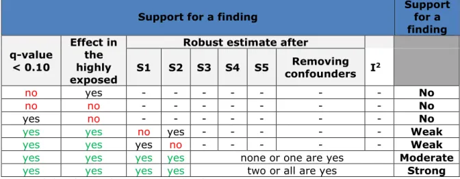
Table 2.5. Criteria for identification and classification of the strength of the support of findings for the mortality outcomes.

Criteria Support for a

finding q-value < 0.10 Effect in the highly exposed

Robust estimate after

I2 Sensitivity 1 (agricultural workers excluded) Sensitivity 2 (restricted to non-urban residents) Removing confounders no yes - - - - No no no - - - - No yes no - - - - No

yes yes no - - - Weak

yes yes yes none or one are yes Moderate

yes yes yes two or all are yes Strong

Table 2.6. Criteria for identification and classification of the strength of the support of findings for the Health Monitor data set.

Criteria Support for a

finding q-value < 0.10 Effect in the highly exposed

Robust estimate after

I2 Sensitivity 1 (individuals with urbanization degree 3 excluded) Sensitivity 2 (restricted to non-urban residents) Removing confounders no yes - - - - No no no - - - - No yes no - - - - No

yes yes none or one are yes Moderate

Table 2.7. Criteria for identification and classification of the strength of the support of findings for the perinatal outcomes.

Support for a finding Support for a finding q-value < 0.10 Effect in the highly exposed

Robust estimate after

S1 S2 S3 S4 S5 _{confounders I}Removing 2

no yes - - - No

no no - - - No

yes no - - - No

yes yes no yes - - - Weak

yes yes yes no - - - Weak

yes yes yes yes none or one are yes Moderate

yes yes yes yes two or all are yes Strong

S1: excluded mothers working in the agricultural setting

S2: excluded mothers and fathers working in the agricultural setting S3: restricted to mothers living in non-urban neighbourhoods S4: excluded non-Dutch mothers

S5: excluded mothers that changed address during pregnancy

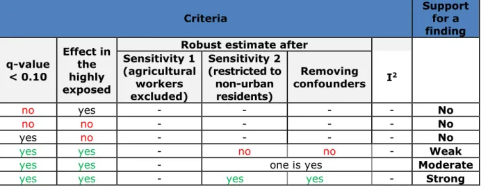
Table 2.8. Criteria for identification and classification of the strength of the support of findings for the EHR data.

Criteria Support for a

finding q-value < 0.10 Effect in the highly exposed

Robust estimate after Sensitivity 1 (agricultural workers excluded) Sensitivity 2 (restricted to non-urban residents) Removing confounders I2 no yes - - - - No no no - - - - No yes no - - - - No

yes yes - no - - Weak

Table 2.9. Criteria for identification and classification of the strength of the support of findings for the questionnaire data.

2.8 Re-analysis of mortality outcomes

We used an updated database of DUELS for the mortality outcomes. The most important difference was that the original method for selecting those who did not move in the period 1995-2003 was too conservative. As a result, the new database contained 3.1 million persons, as

compared to 2.3 million in the first survey.

We repeated the analyses following the original analytical approach (see chapter 8 of the first report; Simões et al., 2018). Four epidemiologists compared independently the heat maps (see Figure 8.4 of the first report) of the new and old results, and indicated which particular crop-outcome combinations should be further explored.

Criteria Support for a

finding q-value < 0.10 Effect in the highly exposed

Robust estimate after Sensitivity 1 (agricultural workers excluded) Sensitivity 2 (restricted to non-urban residents) Removing confounders I2 no yes - - - - No no no - - - - No yes no - - - - No

yes yes - no no - Weak

yes yes - one is yes Moderate

3

Results

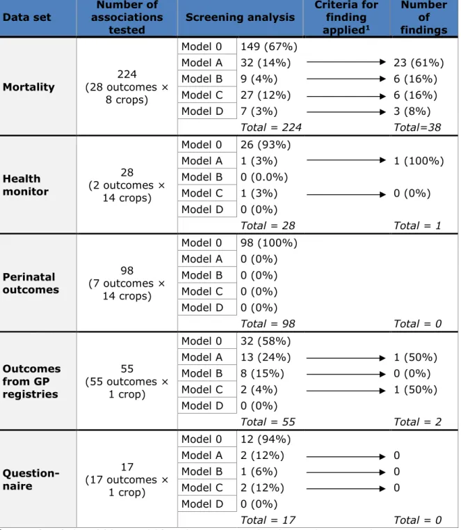
Table 3.1 summarises the results of the screening analysis and the number of findings obtained from the analysis of each data set explored in this report. In total there were 41 findings, all having strong support lent by the robustness of the estimates in the additional analyses. All independent epidemiologists agreed that estimates were robust. 3.1 Total and cause-specific mortality

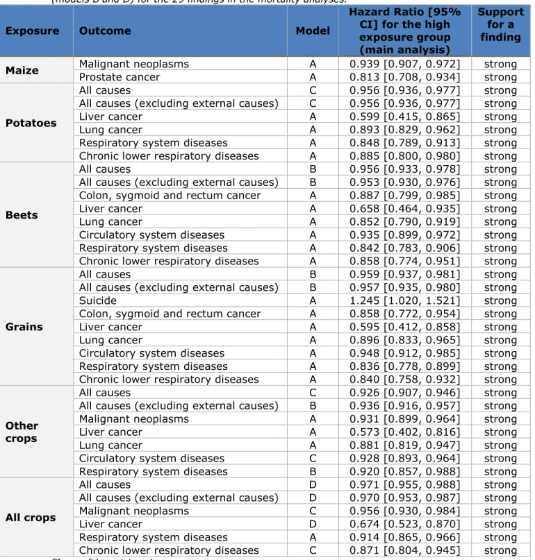
We tested a total of 224 associations (exposure-outcome pairs) for which 149 (67%) model 0 was the best model (Appendix 1a). Of the 75 models that had models A, B, C or D as best model, 38 met the two criteria for being a finding (q-value of the screening model <0.1 and significant effect in the highly exposed in the main model). The results of the main analysis for these findings are presented in Table 3.2. All but one of the 38

findings indicated a decreased hazard for a specific cause of death in the highly exposed compared to the unexposed (n=28) or the low exposure group (n=9). Only the exposure to grains yielded an increased hazard for death from suicide in the highly exposed compared to the unexposed. For most findings (76%), the screening analysis showed a linear relationship between the outcome and the exposure, and all were considered to

provide strong support for a finding. The estimates from the main analysis did not change considerably after the sensitivity analyses and the removal of the confounders from the model (Appendix 2a). The estimates did not show high heterogeneity among the four regions of the Netherlands either.

The analyses where we included the area of (specific) crop between 250m and 500m (donut analysis) showed that the estimate of the 250m buffer from the main analysis changed more than 10% in 12 (32%) of the 38 findings. Of these, only two yielded an estimate that was further away from the null than the estimate of the main analysis. The estimate obtained for the donut itself refers to the change in hazard per 1 hectare increase in area of crop (continuous variable). For ease of interpretation, we calculated the range between the 10th and 90th percentiles of the exposure and report its estimated hazard ratio. In general, the hazard ratio for the donuts are close to null. The results of the donut analyses are presented in Appendix 2a.

Table 3.1. Summary table of the results of the screening analysis and the findings across the five data sets studied.

Data set associations Number of

tested Screening analysis

Criteria for finding applied1 Number of findings Mortality (28 outcomes × 224 8 crops) Model 0 149 (67%) Model A 32 (14%) 23 (61%) Model B 9 (4%) 6 (16%) Model C 27 (12%) 6 (16%) Model D 7 (3%) 3 (8%) Total = 224 Total=38 Health monitor 28 (2 outcomes × 14 crops) Model 0 26 (93%) Model A 1 (3%) 1 (100%) Model B 0 (0.0%) Model C 1 (3%) 0 (0%) Model D 0 (0%) Total = 28 Total = 1 Perinatal outcomes 98 (7 outcomes × 14 crops) Model 0 98 (100%) Model A 0 (0%) Model B 0 (0%) Model C 0 (0%) Model D 0 (0%) Total = 98 Total = 0 Outcomes from GP registries 55 (55 outcomes × 1 crop) Model 0 32 (58%) Model A 13 (24%) 1 (50%) Model B 8 (15%) 0 (0%) Model C 2 (4%) 1 (50%) Model D 0 (0%) Total = 55 Total = 2 Question-naire 17 (17 outcomes × 1 crop) Model 0 12 (94%) Model A 2 (12%) 0 Model B 1 (6%) 0 Model C 2 (12%) 0 Model D 0 (0%) Total = 17 Total = 0

1 _{Criteria for a finding: (a) best model from the screening analysis has q-value < 0.1 and}

(b) statistically significant effect in the highly exposed in the main (categorical) analysis Model 0: model without the exposure variable

Model A: model with the exposure as a continuous variable

Model B: model with the exposure as a continuous variable and a dummy variable for the unexposed group

Model C: model with a spline term on the continuous exposure variable

Model D: model with a spline term on the continuous exposure variable and a dummy variable for the unexposed group

Table 3.2. Hazard ratio and 95% confidence interval of the highly exposed group compared to the unexposed group (models A and C) or the low exposed group (models B and D) for the 29 findings in the mortality analyses.

Exposure Outcome Model

Hazard Ratio [95% CI] for the high exposure group (main analysis)

Support for a finding Maize Malignant neoplasms _{Prostate cancer} A _A 0.939 [0.907, 0.972] _{0.813 [0.708, 0.934]} strong _strong

Potatoes

All causes C 0.956 [0.936, 0.977] strong

All causes (excluding external causes) C 0.956 [0.936, 0.977] strong

Liver cancer A 0.599 [0.415, 0.865] strong

Lung cancer A 0.893 [0.829, 0.962] strong

Respiratory system diseases A 0.848 [0.789, 0.913] strong

Chronic lower respiratory diseases A 0.885 [0.800, 0.980] strong

Beets

All causes B 0.956 [0.933, 0.978] strong

All causes (excluding external causes) B 0.953 [0.930, 0.976] strong

Colon, sygmoid and rectum cancer A 0.887 [0.799, 0.985] strong

Liver cancer A 0.658 [0.464, 0.935] strong

Lung cancer A 0.852 [0.790, 0.919] strong

Circulatory system diseases A 0.935 [0.899, 0.972] strong

Respiratory system diseases A 0.842 [0.783, 0.906] strong

Chronic lower respiratory diseases A 0.858 [0.774, 0.951] strong

Grains

All causes B 0.959 [0.937, 0.981] strong

All causes (excluding external causes) B 0.957 [0.935, 0.980] strong

Suicide A 1.245 [1.020, 1.521] strong

Colon, sygmoid and rectum cancer A 0.858 [0.772, 0.954] strong

Liver cancer A 0.595 [0.412, 0.858] strong

Lung cancer A 0.896 [0.833, 0.965] strong

Circulatory system diseases A 0.948 [0.912, 0.985] strong

Respiratory system diseases A 0.836 [0.778, 0.899] strong

Chronic lower respiratory diseases A 0.840 [0.758, 0.932] strong

Other crops

All causes C 0.926 [0.907, 0.946] strong

All causes (excluding external causes) B 0.936 [0.916, 0.957] strong

Malignant neoplasms A 0.931 [0.899, 0.964] strong

Liver cancer A 0.573 [0.402, 0.816] strong

Lung cancer A 0.881 [0.819, 0.947] strong

Circulatory system diseases C 0.928 [0.893, 0.964] strong

Respiratory system diseases B 0.920 [0.857, 0.988] strong

All crops

All causes D 0.971 [0.955, 0.988] strong

All causes (excluding external causes) D 0.970 [0.953, 0.987] strong

Malignant neoplasms C 0.956 [0.930, 0.984] strong

Liver cancer D 0.674 [0.523, 0.870] strong

Respiratory system diseases A 0.914 [0.865, 0.966] strong

Chronic lower respiratory diseases C 0.871 [0.804, 0.945] strong

CI = confidence interval

Model 0: model without the exposure variable

Model A: model with the exposure as a continuous variable

Model B: model with the exposure as a continuous variable and a dummy variable for the unexposed group

Model C: model with a spline term on the continuous exposure variable

Model D: model with a spline term on the continuous exposure variable and a dummy variable for the unexposed group

3.1.1 Association between grains and suicide mortality

Table 3.3 shows the estimates obtained for the analyses studying the association between death by suicide and living within 250m of grain crops, the only finding that indicated a higher risk of death. The estimate for the highly exposed group is robust across the several additional analyses performed, with no significant heterogeneity across the four regions.

Table 3.3. Estimates obtained for the highly exposed group in the main and additional analyses conducted for the association between death by suicide and living within 250m of grain crops.

Suicide and Grains Estimate of top 10% exposed _{[95% CI]} Main analysis (HR [95% CI]) 1.245 [1.020, 1.521]†

Sensitivity analyses (HR [95% CI]) Agricultural workers excluded 1.223 [0.991, 1.509] Restricted to people living in non-urban neighbourhoods 1.205 [0.971, 1.497] Basic model1 _{(HR [95% CI]) 1.304 [1.073, 1.585]†}

Donut analysis (HR [95% CI]) 1.098 [0.807, 1.493]

Region heterogeneity (I2_{) 57%}

† Significant after FDR correction (q-value < 0.10) 1 Controlled only for sex

CI = confidence interval

3.1.2 Re-analysis using the original method

Repeating the analyses of mortality using the updated database

following the original analytical approach yielded similar and consistent findings as compared with those reported in Simões et al., 2018. Importantly, the association between living near maize and mortality from chronic lower respiratory diseases (predominantly COPD) remained a finding after additional analyses. In addition, the observation that living near fields with the rotating crops potatoes, beets and grains coincided with an increased mortality due to leukaemia remained noteworthy.

3.2 Health Monitor outcomes

Of the 28 associations tested, only two had models A, B, C or D as best model (Appendix 1b). From these, one showed a significant effect in the high exposure group in the main analysis. This finding showed decreased odds of having poor perceived health when living within 250m of potato seeds crops when comparing the highly exposed to the unexposed (Odds Ratio [95% confidence interval] = 0.933 [0.891, 0.978]). This association was linear and strongly supported by the sensitivity analyses

(Appendix 2b) and the analysis without the confounders. Heterogeneity was also low among the four regions of the Netherlands.

3.3 Perinatal outcomes

The model screening analyses yielded model 0 as the best model for all 98 associations tested, revealing that the birth outcomes were not associated with having specific types of crops within 250m from the mothers’ residences. We therefore did not conduct any further analyses. 3.4 Nivel Electronic Health Records from GP registries

Model 0 was identified as the best model for almost 60% of the investigated outcomes. Only two findings were observed (Table 3.4). These showed decreased odds of being prescribed with medication for respiratory health problems and those of the nervous system when living within 250m from fruit crops, when comparing the highly exposed to the unexposed. Results did not change after excluding participants living in moderately urbanized areas (OR 0.86 (0.78-0.95) and 0.79 (0.71-0.88), respectively). However, given that it was only feasible to adjust for a basic set of confounders and, consequently, a limited range of sensitivity analyses (Appendix 2d), we considered the support for these findings as moderate.

Table 3.4. Odds ratio and 95% confidence interval of the exposed group compared to the unexposed group (models A and C) or the low exposed group (models B and D) for the two findings.

Exposure Outcome Model

Odds Ratio [95% CI] for the high exposure group (main analysis) Support for a finding Fruit Medication for respiratory system A 0.86 [0.78, 0.94] Moderate Medication for

nervous system C 0.78 [0.71, 0.87] Moderate

CI = confidence interval

Model A: model with the exposure as a continuous variable

Model C: model with a spline term on the continuous exposure variable

3.5 Nivel questionnaire survey

The model screening analyses yielded model 0 as the best model for 70% of the examined outcomes and no findings were identified (Appendix 1e). Therefore, no further analyses were performed.

4

Discussion

In this study, we expanded on our previous analyses where we assessed the associations between living in proximity of agricultural plots and various health outcomes (Simões et al., 2018). In contrast to our previous analyses, we did not assume a strong gradient of the associations with distance to the crop, as the assumption of a clear exposure gradient by distance was not supported by the results of the OBO exposure study. The concern was that, possibly, relevant

associations with health had been overlooked. Therefore in this analysis, we focused on possible associations for living within 250m from

agricultural plots, while evaluating the same set of health outcomes as in the previous report. We nevertheless used strict statistical criteria and performed additional sensitivity analyses. In general, our results support the findings presented in the previous report. People who lived nearer to agricultural plots appeared, in general, to be slightly healthier than people who lived further away.

Almost all (31) of the 32 findings (of the 422 crop-outcome combinations studied) showed reduced risks for adverse health outcomes in people living within 250m distance from certain crops compared to those who lived further away. This was consistent for different regions of the Netherlands, and remained apparent after limiting the analyses to non-agricultural occupations and non-urban neighbourhoods

(<1,000 addresses/km2_{). The fact that the majority of the observed}

associations showed reduced risks may indicate residual confounding, for example due to lack of relevant individual lifestyle-related information such as smoking, alcohol consumption, and/or physical activity in the mortality and GP registry data sets.

In contrast, as the only finding with an increased risk, we observed a higher mortality due to suicide among people living in the proximity of grain fields. This was consistent for different regions, and further

supported by sensitivity analyses limited to non-agricultural occupations and non-urban neighbourhoods. Given the inherent limitations of the data, it was not possible to clarify which specific factors may underly this association that was possibly a chance finding.

Re-analyses of mortality using the original method and the updated, larger database confirmed the earlier finding that risk of mortality from chronic lower respiratory diseases (predominantly COPD) was higher in people living near maize fields. We also confirmed the noteworthy association between living near field with rotating crops potatoes, beets and grains and mortality due to leukaemia.

The overall limitations discussed in the first report remain relevant here. Major issues to be highlighted are the lack of information on individual exposure to specific pesticides and, in most analyses, the lack of lifestyle and other factors that could have led to (residual) confounding.

Conclusion

The results from these additional analyses are in agreement with the overall findings of the first study. The added value is the reassurance that our previous methodology was sound and we did not miss any findings by using different assumptions and criteria. Two different agnostic approaches led to the same conclusions. Studies based on different data sources and other methodology are needed to more specifically study potential adverse health effects of residential exposure to pesticides in people living in the vicinity of agricultural plots.

Recommendations for further study

The main recommendation is to perform studies that improve on the assessment of exposure to specific pesticides, including mixtures. In addition, we recommend targeting specific health outcomes of concern. The findings for specific health outcomes associated with exposure to pesticides in our and previous studies require further study. Such research should focus on COPD and other health problems that are regularly mentioned in the scientific literature, such as leukaemia, Parkinson’s disease and cognitive effects. Finally, future studies should include a broader set of potentially confounding factors including but not limited to lifestyle, in order to improve interpretation of the findings.

5

References

Benjamini, Y., & Hochberg, Y. (1995). Controlling the False Discovery Rate: A Practical and Powerful Approach to Multiple Testing. Journal of the Royal Statistical Society. Series B (Methodological), 57(1), 289–300.

Retrieved from http://www.jstor.org/stable/2346101

Higgins, J.P.T., Thomas, J., Chandler, J., Cumpston, M., Li, T., Page, M.J., Welch, V.A. (editors). Cochrane Handbook for Systematic Reviews of Interventions version 6.0 (updated July 2019). Cochrane, 2019.

Available from www.training.cochrane.org/handbook

Raftery, A. E. (1995). Bayesian Model Selection in Social Research. Sociological Methodology, 25, 111–163.

https://doi.org/10.2307/271063

Simões, M., Brouwer, M., Krop, E., Huss, A., Vermeulen, R.C.H., Baliatsas, C., IJzermans, J., Verheij, R., Janssen, N., Marra, M., Wijga, A.H. & Rietveld, A.G. (2018). Gezondheidsverkenning omwonenden van landbouwpercelen.

https://www.rivm.nl/bibliotheek/rapporten/2018-0068.pdf

Vermeulen, R.C.H., Gooijer, Y.M., Hoftijser, G.W., Lageschaar, L.C.C., Figueiredo, D.M., Huss, A., Krop, E.J.M., Oerlemans, A.,

Scheepers, P.T.J., Berg, F. van den, Holterman, H.J., Jacobs, C.J.M., Kruijne, R., Mol, J.G.J., Wenneker, M., Zande, J.C. van de, Kivits, C.M., Duyzer, J., Gerritsen-Ebben, M.G. & Sauer, P.J.J. (2019). Research on exposure of residents to pesticides in the Netherlands. https://www.bestrijdingsmiddelen-omwonenden.nl/english

6

Appendices

1. Overview of the models (0, A, B, C or D) that best explained the association between the explored outcomes exposure (crop) pair for the five blocks of outcomes

2. Results of additional analyses 3. Glossary

Appendix 1 Overview of the models (0, A, B, C or D) that best explained the association between the

explored outcomes exposure (crop) pair

a) Total and cause-specific mortality Outcome

(cause specific mortality)

Best model

Maize Potatoes Beets Grains Other Crops Fruits Flower Bulbs All Crops

All causes 0 C B B C 0 0 D

All causes (excluding external

causes) 0 C B B B 0 0 D

All external causes 0 C 0 0 0 0 0 0

Traffic accidents 0 0 0 0 A C C D

Other accidents 0 0 D 0 C 0 0 0

Suicide 0 0 0 A 0 0 0 0

Malignant neoplasms A 0 0 0 A 0 0 C

Stomach cancer C C C 0 0 0 0 0

Colon, sygmoid and rectum

cancer D A A A C 0 0 A Liver cancer C A A A A 0 0 D Pancreas cancer 0 0 0 0 0 0 0 0 Lung cancer 0 A A A A 0 0 0 Skin cancer 0 0 0 0 0 0 0 0 Breast cancer 0 C 0 0 0 0 0 0 Ovary cancer 0 0 0 0 0 0 0 C Prostate cancer A 0 0 0 0 0 0 C Kidney cancer 0 0 0 0 0 B C C

Non-Hodgkin lymphoma 0 0 0 0 0 0 0 0

Brain cancer 0 0 0 0 C C D 0

Leukaemia 0 0 C 0 C 0 0 0

Endocrine, nutritional and

metabolic diseases 0 0 0 0 C 0 0 0

Parkinson's disease 0 0 0 0 0 0 0 A

Alzheimer's disease 0 A A C C 0 0 0

Circulatory system diseases A A A A C 0 0 0

Ischemic heart diseases 0 0 0 0 0 0 0 0

Cerebrovascular diseases 0 0 0 0 0 0 0 0

Respiratory system diseases B A A A B 0 0 A

Chronic lower respiratory

diseases B A A A A 0 0 C

Model type Model 0 Model A Model B Model C Model D

Number of models 149 (67%) 32 (14%) 9 (4%) 27 (12%) 7 (3%) Legend HR<1 Support for a finding HR>1 no weak moderate strong HR = hazard ratio

Health monitor Outcome Best model M aiz e W in te r w h ea t S u m m er b arl ey S u mme r w h ea t O th er c er ea ls Po ta to es (c ons um pt io n) Po ta to es (st arc h ) Po ta to es (se ed li n g s) B eet s Or na me nt al p la nt s, t ree n u rs er ie s V eg et ab le s Fr u it Fl o w er b u lb s Al l c ro p s Anxiety / Depression 0 0 0 0 C 0 0 0 0 0 0 0 0 0 Perceived health 0 0 0 0 0 0 0 A 0 0 0 0 0 0 Model type 0 A B C D Number of models 26 (93%) 1 (4%) 0 (0%) 1 (4%) 0 (0%) Legend

OR<1 Support for _{a finding OR>1} no weak moderate strong OR = Odds Ratio b) Perinatal outcomes

The best model was 0 for all 98 combinations of 14 crops and 7

pregnancy/birth outcomes. For details see chapter 4 of the first report (Simões et al., 2018).

c) Outcomes from GP registries

Outcome Best model _{Fruit crops}

C h ro n ic c o n d it io n s Asthma 0 Multiple sclerosis 0 Ulcerative colitis 0 Hyper-/Hypothyroidism 0 Hodgkin's disease A Leukaemia 0 Malignant neoplasms 0 Anxiety 0 Depression B Autism A ADHD 0 Infertility 0 COPD B Lung cancer 0

Coronary heart disease 0

Heart failure A

Hypertension 0

Diabetes B

Parkinson's disease C

Congenital abnormalities 0

Genital birth defects 0

A cu te s ym pt om s/ con di ti o n s an d in fe cti o n s Fatigue/Tiredness 0 Abdominal/Stomach symptoms A Nausea B Diarrhoea/constipation 0 Eye irritation 0

Pain or pressure in chest 0

Heat palpitations A Headache 0 Dizziness 0 Sleep problems A Memory/concentration problems 0 Psychological symptoms A Cough B Shortness of breath 0 Skin symptoms A

Upper respiratory tract

infection A Sinusitis 0 Acute bronchitis/bronchiolitis A Influenza 0 Pneumonia A Q-fever/allergic rhinitis 0 Gastro-enteritis 0 Conjunctivitis A Respiratory symptoms B