DISJUNCTIVE ARCS AND RESOURCE
FLOWS IN PROJECT NETWORKS
Aantal woorden / Word count: < 16.569 >
Henk Vanderjeugt
Stamnummer / student number : 01507498
Promotor / supervisor: Prof. Dr. Mario Vanhoucke
Masterproef voorgedragen tot het bekomen van de graad van: Master’s Dissertation submitted to obtain the degree of:
Master in Business Engineering: Operations Management
This page is not available because it contains personal information.
Ghent University, Library, 2021.
The primary aim of this thesis study is to investigate how an approach based on resource flows may help to solve the Resource Constrained Project Scheduling Prob-lem (RCPSP), which has the challenge to find precedence and resource feasible com-pletion times for all activities such that the total makespan of a project is minimised.
For this objective, the Disjunctive Graph (DG) model, which is originally be ap-plied to the Job-shop Scheduling Problem (JSP), is extended and apap-plied to the more complex RCPSP.
After an overview of existing literature has been pointed out, an attempt is made to transform these theoretical insights into a practical method, after which the strengths and weaknesses are experimentally investigated by means of a Java project.
In addition to the regular time objective, investigation has been done into how this resource flow based scheduling technique performs on other non-regular project objectives, such as ensuring work continuity of resources and ensuring resource lev-eling.
This master’s dissertation is the final part of a 5-year trajectory with the aim to obtain the degree of Master of Science in Business Engineering: Operations Manage-ment. With gratitude and satisfaction I reflect back on my period at the University of Ghent, in which I was strongly inspired by the enthusiasm and solution-oriented thinking of my promotor prof. dr. Mario Vanhoucke.
Although this master’s dissertation was written in very exceptional times due to the COVID-19 outbreak, it hardly influenced the outcome of my research. This is the result of a very flexible approach of my mentor and PhD-candidate Rob Van Eynde, who was willing to share his excellent knowledge with me via several video chat sessions. I am very grateful to him.
In addition to this, I would like to thank my parents and girlfriend for the un-conditional support they have given me during this period. Thank you all.
List of Abbreviations viii
I
Introduction
1
1 An Introduction to Resource Constrained Project Scheduling 2
1.1 Problem Formulation . . . 2
1.2 Time Complexity . . . 4
1.3 A Popular Solution Approach . . . 5
2 A Resource Flow Based Solution Approach 6 2.1 Job-shop Scheduling . . . 7
2.1.1 Job-shop Scheduling on the Disjunctive Graph . . . 7
2.1.2 Local Search Techniques . . . 10
2.2 Resource Constrained Project Scheduling . . . 13
2.2.1 Relationship with JSP and Previous Work . . . 14
2.2.2 RCPS on the Disjunctive Graph . . . 15
2.3 Resource Flow-based MILP Formulation . . . 17
2.4 AON Flow Network . . . 20
2.5 Neighbourhood Structure . . . 20
2.5.1 Reverse Neighbourhood . . . 21
2.5.2 Reroute Neighbourhood . . . 26
II
Methodology
28
3.1 Methodology . . . 29
3.1.1 Initial Solution Generation . . . 31
3.1.2 Solution Modification Process . . . 41
3.1.3 Heuristics . . . 61
III
Results and Conclusion
66
4 Results 67 4.1 Design Choices . . . 674.1.1 Neighbourhood Sizes . . . 68
4.1.2 Operators . . . 73
4.1.3 Parameter Tuning . . . 78
4.1.4 Multiple Seeds Strategy . . . 80
4.1.5 Design Summary . . . 82
4.2 Performance Analysis . . . 84
4.2.1 Average number of technological predecessors per activity . . 84
4.2.2 Number of resource types needed by an activity . . . 85
4.2.3 Availability of resources . . . 86
4.3 Non Regular Objectives . . . 87
4.3.1 Ensuring Work Continuity of Resources . . . 87
4.3.2 Resource Leveling Project Scheduling Problem . . . 88
A Set containing all technological precedence relations ESi Earliest starting time of activity i
LFi Latest finishing time of activity i
Rk Available number of resource units of resource type k V Set containing all real activities
V∗ Set containing all real activities and activity n + 1 V0 Set containing all real activities and activity 0
Vall Set containing all real activities, activity 0 and activity n + 1 ci Completion/Finishing time of activity i
fi,j,k Number of resource units transferred from activity i to activity j of resource type k
n Number of (real) activities included in a project pi Processing time of activity i
r Number of different resource types
rik Resource requirement of activity i for resource k si Starting time of activity i
AON Activity On Node
JSP Job-shop Scheduling Problem
MILP Mixed Integer Linear Program
NP Nondeterministic polynomial time
1.1 AON Network . . . 4
2.1 Job-shop Scheduling on the Disjunctive Graph . . . 9
2.2 Possible solution on Disjunctive Graph . . . 9
2.3 Modified solution on Disjunctive Graph . . . 13
2.4 Project Scheduling on the Disjunctive Graph . . . 16
2.5 Possible solution on the Disjunctive Graph . . . 16
2.6 AON Flow Network . . . 20
2.7 Before Reverse Modification (1) . . . 22
2.8 After Reverse Modification (1) . . . 22
2.9 Before Reverse Modification (2) . . . 24
2.10 After Reverse Modification (2) . . . 25
2.11 Before Reroute Modification . . . 27
2.12 After Reroute Modification . . . 27
3.1 Case Study: Network diagram . . . 31
3.2 Flowchart Symbols . . . 32
3.3 Initial Solution Generation Process . . . 32
3.4 Gantt Chart: Initial Project Schedule . . . 36
3.5 Case Study: Initial resource flow generation (1) . . . 38
3.6 Case Study: Initial resource flow generation (2) . . . 40
3.7 Case Study: Initial resource flow generation (3) . . . 41
3.8 Case Study: Initial resource flow generation (4) . . . 41
3.9 Case Study: Initial resource flow generation (5) . . . 42
3.10 Case Study: Complete Initial Resource Flow (Resource 1) . . . 42
3.12 Solution Modification Process . . . 44
3.13 Non critical resource transfer between a pair of critical activities . . 45
3.14 Critical Arcs in Initial Solution . . . 49
3.15 Before Reverse Modification . . . 51
3.16 After Reverse Modification . . . 51
3.17 Modified Adjacency Matrix Resource Flow 2 . . . 51
3.18 Forbidden Resource Flows in Reroute Modifications . . . 53
3.19 Before Reroute Modification . . . 54
3.20 After Reroute Modification . . . 54
3.21 Modified Adjacency Matrix Resource Flow 1 . . . 55
3.22 Best Found Resource Flow 1 . . . 64
3.23 Best Found Resource Flow 2 . . . 64
3.24 Gant Chartt: Best Generated Schedule . . . 65
4.1 Deciding upon neighbourhood sizes (4%) . . . 72
4.2 Deciding upon neighbourhood sizes (Opt.%) . . . 72
4.3 Identifying Desirable Reroute Modification (1) . . . 74
4.4 Identifying Desirable Reroute Modification (2) . . . 74
4.5 Identifying Desirable Reverse Modification (1) . . . 76
4.6 Identifying Desirable Reverse Modification (2) . . . 77
4.7 Impact of varying P(Reroute) . . . 79
4.8 Impact of Design Options on 4% . . . 82
4.9 Impact of Design Options on Opt. % . . . 83
4.10 Impact of Average number of technological predecessors per activity . 85 4.11 Impact of Number of resource types needed by an activity . . . 86
3.1 Case Study: Project Overview . . . 30
3.2 Case Study: Resource Availabilities . . . 31
3.3 Critical Activities in Initial Solution . . . 50
3.4 Case Study: Minimal Time Distances between Activities . . . 57
3.5 Case Study: Longest Time Paths between Activities . . . 60
3.6 Case Study: Parameter Setting . . . 63
4.1 (Opt-) Connectivity of Neighbourhood Reductions . . . 70
4.2 Neighbourhood Notation . . . 71
4.3 Parameter Setting . . . 71
4.4 Test Results after Updating Operators . . . 78
4.5 Test Results after Parameter Tuning . . . 80
4.6 Multiple Seeds Results . . . 81
4.7 Best Initial Solutions . . . 82
4.8 Improvement Work Continuity . . . 88
1 Parallel Schedule Generation Scheme . . . 35
2 Generate resource flow from schedule . . . 39
3 Generate critical activities . . . 46
4 Generate critical arcs . . . 47
5 Reverse Modification . . . 48
6 Generate Set of Feasible Partners . . . 53
7 Generate distance matrix . . . 56
8 Generate longest paths . . . 58
An Introduction to Resource
Constrained Project Scheduling
Over the years, Resource Constrained Project Scheduling has already generated a lot of interest from many researchers. The aim of this chapter is to introduce the reader to this complex domain of research.
Chapter 1 is structured as follows: first the Resource Constrained Project Scheduling Problem is explained after which the complexity of the problem will be discussed. Finally, some limited insights are provided into a popular solution approach to solve the RCPSP.
1.1
Problem Formulation
The classical RCPSP can be introduced using a problem formulation in accordance with Brucker and Knust (2006), Artigues et al.(2003) and Poppenborg(2014).
The RCPSP has the aim to schedule n activities under both precedence and re-source constraints such that the objective function is minimized. In order to process n activities, r renewable resources k = 1, ...,r with limited capacities Rk are avail-able. This means that at any time t, an amount of exactly Rk units of each resource k is available and so, at any time, a maximum amount Rk units of resource k can be consumed by the n activities. Renewable resources may for example be
equip-ment, machines, human workforce, ... To facilitate the problem formulation set V is introduced. Set V = {1, ..., n} contains all activities.
Each activity i ∈ V may require a certain amount of time to be processed and possibly require different resources to be used during processing. The former is called the processing time pi of activity i and the latter is called the resource re-quirement rik for resource k ∈ R of activity i. It is important to note that all resources required by an activity i have to be available during the complete process duration pi.
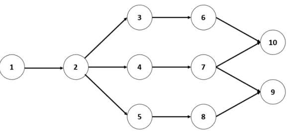
In addition to this, it may be the case that activities must be carried out in a certain order. These relationships between activities inside a project are defined by technological precedence constraints. These constraints are included in set A. A precedence constraint (i, j) ∈ A implies that activity i has to be finished before the start of activity j, with i ∈ V , j ∈ V and i 6= j. One way to visualize all precedence relationships between all activities i ∈ V is by displaying them in an Activity-On-Node (AON) Network. Then, each node represents an activity and each arc i → j refers to a precedence constraint (i, j) ∈ A with i ∈ V and j ∈ V . An example network of ten activities is depicted in figure 1.1.
As already described, the RCPSP’s purpose is to set up a feasible schedule while optimizing the objective. This is done by assigning a starting time si to each activity i ∈ V . Then, the completion time ci of each activity i can be easily calculated by Ci = Si+ pi. Here, preemption is assumed to be not allowed. A schedule S is called a feasible schedule if and only if the schedule is precedence and resource feasible. Hence, at any time t, Sj > Si+ pi has to be respected for all (i, j) ∈ A and at any time t, the sum of resource demands for over all active activities has to be 6 Rk for all k ∈ R. An activity i is called to be active at time t, if activity i is under execution at time t i.e. if Si 6 t < Si+ pi. In addition to this, an optimal sched-ule S∗is referred to be a feasible schedule that optimizes the given objective function.
Figure 1.1: AON Network
end of the project (i.e. the makespan of the project). In other words, this is the same as minimizing the time required to process all activities i = 1, ..., n. Consequently, minimizing Cmax will be the objective function with
Cmax = n max
i=1{Si+ pi}
Hence, the following condition will hold for all feasible schedules S:
Cmax(S∗) 6 Cmax(S)
.
1.2
Time Complexity
Unfortunately, the RCPSP is known to be strongly NP-hard. This can be deduced from the fact that the ’Job-shop Scheduling Problem’ is proved to be NP-hard (Garey, Johnson, and Sethi, 1976). Without going into more detail here, the Job-shop Scheduling Problem can be seen as a less complex case of the Resource Con-strained Project Scheduling Problem. The relationship between these two problem types is later explained in detail in Chapter 2.
Practically, it means when a problem is labeled as NP-hard, it becomes very diffi-cult to arrive at an optimal solution within a reasonable amount of time. Therefore, approximation methods will often be preferred to exact methods, especially when the problem size increases. Approximation methods try to find high quality solutions, that are not necessarily the best, but can be found in a reasonable amount of time.
1.3
A Popular Solution Approach
A well researched group of approximation methods is based on so-called priority rules. The use of priority rules for project scheduling can be explained as follows. Since different activities i ∈ V may compete for the same resource k ∈ R, it may be necessary to delay certain activities in order to obtain a feasible schedule. Then, in order to facilitate the identification of which activities should be scheduled first and consequently, which activities should be delayed, priority rules are applied to order all project’s activities. An example of priority based scheduling is discussed later in the methodology part of this thesis study. Reference is made to section 3.1.1 for this.
A Resource Flow Based Solution
Approach
In Chapter 1, Resource Constrained Project Scheduling was introduced as an NP-hard problem. Because of the high complexity, various solution approaches have already been elaborated. One popular approach is based on the application of pri-ority rules to order project activities.
Alternatively, it is also possible to look at resources as a flow that goes from one ac-tivity to another. This approach is similar to a common used method in the domain of the Job-shop Scheduling Problem (JSP). Therefore, a job-shop scheduling method will be taken as a starting point and will be adapted until it fits the characteristics of the more complex RCPSP.
A well-known and successful solution approach for solving the JSP is based on the Disjunctive Graph (DG) model, which was originally introduced by Roy and Sussmann (1964).
This is why, in the following section, the JSP will be briefly introduced by us-ing the problem formulation of Blazewicz et al. (2000). Next, the disjunctive graph model will be introduced and finally, the original disjunctive graph model will be adapted and applied to resource constrained project scheduling.
During the set up of the resource flow based solution approach, the focus will be on sequencing the activities rather than come up with a schedule. Having said this, it should be clear that once a certain sequence of all activities has been established, a schedule can always be designed by assigning the activities to the corresponding earliest starting times (ESi).
2.1
Job-shop Scheduling
The Job-shop Scheduling problem (or Machine Sequencing problem) is a combina-torial optimization problem in which the challenge is to find the best assignment of operations on machines.
Therefore, the JSP consists out of a set of jobs J ={J1, ..., Jj, ..., Jn} and a set of machines (resources) M = {M1, ..., Mi..., Mm}. Each job Jj is an ordered subset of operations (O) i.e. Jj = {O1, ..., Oo, ..., Op}. Operations inside a job require process-ing on machines in a specified sequence which is denoted by precedence constraints. Moreover, each operation has a processing need on one specific machine and per-forming operations on machines may require a certain processing time, which is here considered as deterministic. Furthermore, only one operation can be processed by a single machine at a certain moment in time which is also known as the capacity constraint.
The traditional objective is here to minimize the total makespan by setting the processing order of all the operations on the available machines while not violating precedence constraints inside jobs and capacity constraints on machines.
2.1.1
Job-shop Scheduling on the Disjunctive Graph
The Disjunctive Graph Model (Roy and Sussmann, 1964) is useful to represent job-shop scheduling problems in an efficient way. The model is characterised by 3 sets (V, A, E) :
1. Set of Vertices (V ):
vertices at the beginning and end of the schedule. The weight of a vertex is equal to the processing time of the corresponding operation except for the dummy vertices which get both a weight of zero.
2. Set of Arcs (A):
The set of arcs connects consecutive operations inside jobs and so expresses technological precedence constraints. In addition to this, extra arcs are added. One arc from the dummy beginning to the first operation of each job and one arc from the last operation of each job to the dummy end. The set of arcs is also called the conjunctive part of the graph.
3. Set of Edges (E):
The set of edges connects all operations requiring processing on the same machine. By way of explanation it can be stated that for every machine, one clique exists that connects all operations requiring processing on that specific resource. Therefore, cliques represent machine chains. This part is referred as the disjunctive part of the graph.
By giving each clique a specific acyclical orientation, a feasible schedule can be devel-oped. Moreover, there exist a one-to-one mapping between any feasible sequencing and sets of choices for the edge orientations (Fortemps and Hapke, 1997). Hence, the set of edges encodes the sequencing decision variables.
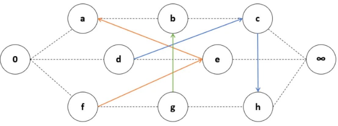
Figure 2.1 is an example (Fortemps and Hapke, 1997) of a disjunctive graph consisting of 3 jobs. The first job (J1) is an ordered subset of Oa → Ob → Oc, the second job (J2) is an ordered subset of Od → Oe and finally, the third job (J3) is an ordered subset of Of → Og → Oh. In other words, the horizontal lines in figure 2.1 all represent technological precedence constraints (i.e. the set of arcs), which set the order of processing inside all jobs.
Besides this, one can also note different cliques in figure 2.1, which consist of opera-tions requiring processing on the same type of machine. In the example, there are 3 cliques which means there are three different machines available. The first machine
Figure 2.1: Job-shop Scheduling on the Disjunctive Graph
(M1) needs to process operations Oa, Oe and Of, the second machine (M2) needs to process operations Ob and Og, while the third machine (M3) needs to process operations Oc, Od and Oh.
Subsequently, the JSP can be solved by finding an orientation for all cliques that minimizes the makespan of all jobs while taking the technological precedence con-straints and capacity concon-straints into account. The makespan is equal to the longest path in the digraph which can be calculated by adding the weights of the correspond-ing vertices. For simplicity, each vertex differcorrespond-ing from the dummy end and beginncorrespond-ing vertex, is here assumed to get a weight of 1.
Figure 2.2: Possible solution on Disjunctive Graph
are oriented as follows: Of → Oe→ Oa, Ob → Og and Od → Oc→ Oh.
Next, one can easily calculate the makespan of this solution by adding the weights of the longest path. In this example, two longest paths can be found, namely, 0 → Od → Oe → Oa → Ob → Oc → Oh → ∞ and 0 → Of → Oe → Oa → Ob → Oc→ Oh → ∞. This results in a makespan of 6 time units.
As appears from the preceding, the disjunctive graph model seems to be able of presenting the JSP in a simple and efficient way, but in addition to this, the dis-junctive graph model also offers opportunities for applying local search techniques (Balas, 1969).
2.1.2
Local Search Techniques
Due to its NP-hard characteristics (Garey, Johnson, and Sethi, 1976 and Sotskov and Shakhlevich, 1995), the JSP is like the RCPSP often solved by use of heuristics. Popular heuristics include local search techniques, which owe their popularity to the fact that they are often able to provide reasonable results in a reasonable amount of time and this for a wide range of problem types. These problem types all have in common that an optimal solution must be found between a set of candidate so-lutions making up together the search space.
Local search algorithms typically start in a certain initial solution state and will iteratively evaluate neighborhood solutions. Solution S’ is said to be a neighbour-ing solution to solution S when it can be obtained by performneighbour-ing a sneighbour-ingle feasible modification to solution S. Next, after evaluating neighbouring solution S0, solution S0 may be accepted as new solution after which the neighbourhood of solution S0 is discovered, evaluated and consequently, a new solution is potentially identified. This process of iteratively evaluating neighbouring solutions continues until a predefined termination criterion is met. Furthermore, only feasible solutions are considered during the search process in this thesis study. With feasible solutions it is referred
to solutions complying with both technological precedence constraints and capacity constraints. In addition to this, only solutions without cycles on the machine chains are considered as feasible since introducing cycles results in allocating multiple times a machine to an operation, which can never be appropriate since preemption is not allowed here.
Moreover, every different local search technique has its own strategy to go through the search space and whether to accept newly discovered solutions. The more ef-ficient the search happens, the more desirable it is. For clarity, efficiency in this context means finding the best possible solution by evaluating as few candidate solutions as possible. Hence, these techniques enable to reduce computational treat-ment to a great extent since only a limited part of the search space is considered. Popular local search algorithms include tabu search and simulated annealing, but many others exist.
Initial Feasible Solution
In order to take off the iterative search process, an initial feasible solution has to be determined. An initial solution can for example be the organisation’s currently used machine sequence schedule or can possibly be generated from scratch by using heuristics. Applied to the JSP, a feasible initial schedule is an acyclic digraph in which the set of machine chains have received a particular orientation.
Neighbourhood
Moreover, the success of local search algorithms is largely determined by the quality of the neighbourhood i.e. the set of solutions that can be obtained from the current solution by performing a single modification. Ideally, the neighbourhood includes solutions with the potential of efficiently leading to a good solution.
Therefore, it must be determined which modifications can be performed to the current solution in order to obtain a neighbouring solution. Here, a strategy may be to guarantee that the obtained neighbouring solution is also part of the set of feasi-ble solutions. Then, a great deal of attention must be paid in determining feasifeasi-ble
modifications.
Since set A contains technological constraints and therefore cannot be adjusted, the scope of research can be limited to modifying arcs on machine chains (i.e. set E). A modification then implies that the orientation of a certain arc is reverted.
Moreover, it is important to understand that not all arcs can be reverted as re-verting arcs may lead to the introduction of cycles. This is why, Fortemps and Hapke (1997) suggest to focus on reverting the set of only arcs.
Arc Ox → Oy belongs to the set of only arcs if Ox → Oy is the only path be-tween Ox and Oy and Ox→ Oy 6∈ A . For example, in the solution shown by figure 2.2, it is not allowed to revert arc Od → Oc, since there exist another path from Od to Oc (namely Od → Oe → Oa → Ob → Oc). Should one still try to revert the orientation of arc Od→ Oc and thus, performing operation Ocbefore operation Od, then cycle Od → Oe → Oa → Ob → Oc → Od is introduced and consequently, the modified solution becomes unfeasible.
Therefore, when carrying out a modification, it must always be checked whether an arc belongs to the set of only arcs. This can be very time consuming since the whole digraph has to be checked each time a modification is carried out. Fortu-nately, Fortemps and Hapke (1997) propose to reduce computational time by only considering a subset of only arcs. This subset is called the set of critical arcs. An arc Ox → Oy is called a critical arc if it is located on the longest path with Ox → Oy 6∈ A. The reasoning to focus only on the set of critical arcs has been justified by three theorems introduced by van Laarhoven et al. (1992).
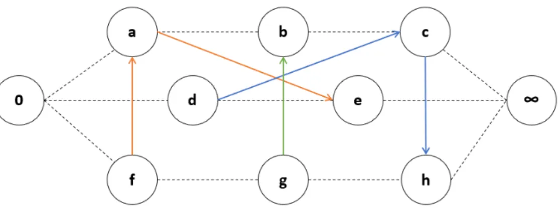
For example in figure 2.2, the following set of critical arcs can be safely reverted Of → Oe, Oe → Oa and Oc → Oh without introducing cycles. If we consider machine chain 1 (Of → Oe → Oa), one can try to revert arc Oe → Oa and thus, perform operation Oa before operation Oe. The machine chain is now modified to Of → Oa→ Oeand the modified disjunctive graph model is represented in figure 2.3.
Again, it is possible to find the longest path and consequently, calculate the the makespan. The longest path is here: 0 → Of → Oa → Ob → Oc → Oh → ∞ resulting in a makespan of 5 time units instead of 6 time units.
Figure 2.3: Modified solution on Disjunctive Graph
By repeating this procedure one can try to arrive at a good solution and save computational time as the search tree can drastically be cut down and storage requirements are limited to the data pertinent to the current solution (Blazewicz, Pesch, and Sterna, 2000).
2.2
Resource Constrained Project Scheduling
Since modifying disjunctive arcs turned out to be a very successful technique for solv-ing the JSP, it is interestsolv-ing to investigate whether this technique can contribute to solving the RCPSP.
Hence, the main objective in this thesis study is to adopt the same approach as with the JSP and thus, to find high quality solutions by iteratively evaluating neighboring solutions obtained by resource flow modifications. Therefore, the Disjunctive Graph model is taken as a starting point and will be extended to the problem specific char-acteristics of the RCPSP.
This is why, first the relationship between these the JSP and RCPSP is described after which a resource flow based scheduling method is elaborated based on insights from previous studies.
2.2.1
Relationship with JSP and Previous Work
As already described, the JSP can be seen as a special case of the more complex RCPSP. It has been indicated by Baker (1974), that the JSP is equivalent with a RCPSP where only one resource unit (i.e. one machine) is required by all activities i ∈ V (i.e. operation). This is in contrast with the RCPSP, where an activity may require resources from different resource groups and in different amounts.
In order to denote the amount of resource units transferred from one activity to another, an extended DG model has been proposed by Fortemps and Hapke (1997), which is heavily inspired by reversing critical arcs on the DG model for the JSP. They indicate reversing a critical arc as a Serial Modification. In addition to revers-ing arcs, the opportunity was demonstrated for a second type of modification, which was denoted as a Parallel Modification. These modifications were only sketched leav-ing room for further investigation.
Next, Artigues et al. (2003) came up with an alternative Mixed Integer Linear Programming formulation for the RCPSP. This approach was heavily focused on resource flows and so, provided useful insights for the elaboration of a solution ap-proach based on resource flow modifications.
Furthermore, an attempt was already made to apply the proposed resource flow modifications by Fortemps and Hapke (1997) in combination with insights from Ar-tigues’ et al. (2003) MILP formulation. This research was done by Poppenborg (2014) where project scheduling techniques were applied to a hospital evacuation planning. This research served as starting point for this thesis study.
2.2.2
RCPS on the Disjunctive Graph
For the objective of elaborating a resource flow based scheduling method, the DG model as proposed by Fortemps and Hapke (1997) is explained first. Here, in simi-larity with the original Disjunctive Graph model, the extended version can be char-acterised by 3 sets (V, A, E):
1. Set of Vertices (V ):
The set of vertices contains a node for each activity as well as two dummy vertices at the beginning and end of the schedule. In contrast to the orig-inal DG model, two extra nodes are added for each resource group. One representing the initial resource disponibility and one representing the final resource disponibility. As this thesis is focused on renewable resources, the initial disponibility should always be equal to the final disponibility.
2. Set of Arcs (A):
The set of arcs expresses technological precedence constraints. The novelty here is that some extra arcs have been added. One extra arc from each resource group’s beginning to each consuming activity and another extra arc from each consuming activity to each resource group’s end. An activity i is called a consuming activity of resource group k, if activity i requires resource k for processing.
3. Set of Edges (E):
The set of edges connects all activities requiring the same resource type and can be compared with machine chains defined in the JSP. Nevertheless, this set includes the more complex resource chains. For each resource type k ∈ R, a resource chain is identified. Since activities may require multiple resource types, two activities can be linked by several edges.
Different from the JSP, a feasible schedule can here be developed by defining for each resource chain how resource units are transferred from one activity to another. Hereby, the key will be in determining for all consuming activities one or more re-source successors and the amount of transferred units.
The above may perhaps be clarified with an example (Fortemps and Hapke, 1997). Figure 2.4 presents a project consisting out of three activities (activity a, activity b and activity c). Here, there is only one resource chain (green lines), so there is only one resource type available and required by the activities. Consequently, only one resource group beginning and only one resource group end is included in figure 2.4. Furthermore, there are no precedence constraints (gray lines) between the activities.
Then, a possible solution can be developed by setting up a resource flow dia-Figure 2.4: Project Scheduling on the Disjunctive Graph
gram. This is shown in figure 2.5. Here, the required resource units are as follow: 3, 2 and 2 for respectively activity a, activity b and activity c. The resource avail-ability is 4. Therefore, 4 resource units are initially stored in the resource group beginning. Here, activity a is the first activity to be executed and so, activity a receives 3 resource units from the resource group beginning.
After activity a has been completed, 2 resource units are transferred from activity Figure 2.5: Possible solution on the Disjunctive Graph
a to activity b and 1 resource unit is passed immediately to the resource group end. After the completion of activity b, 2 units are passed to activity c. Finally, 2 units
are passed from activity c to the resource group end.
Note that 1 resource unit is passed immediately from the resource group begin-ning to the resource group end. This means that 1 resource unit is not used by any activity during the project’s duration.
Here, all activities are sequentially executed since an activity i can only be exe-cuted if all of its resource requirements rik are satisfied. Consequently, assuming all activities have a process duration of 1 time unit, activity a is executed from time unit 0 to 1, activity b is executed from time unit 1 to 2 and activity c is executed from time unit 2 to 3.
Despite the simplicity of the example it was shown what the focus will be on. Namely, by focusing on resource flows, activities can be sequenced. Then, it is possible to come up with a solution schedule for the RCPSP by assigning an ear-liest starting time to all activities i ∈ V . Moreover, it is possible to formulate the RCPSP as a resource flow based Mixed-Integer Linear Program. This is the subject of section 2.3.
2.3
Resource Flow-based MILP Formulation
One possible Mixed-Integer Linear Programming (MILP) formulation for the RCPSP has been developed by Artigues et al. (2003) and focuses on resource feasible flows between project activities.
A resource feasible flow entails that for all activities i ∈ V and for all resources k ∈ R, the amount of incoming resource units and the amount of outgoing resource units, is equal to resource requirement rik. Besides this, a resource feasible flow has to be acyclic and should not violate any precedence constraint. If these conditions are satisfied, one can speak of a resource feasible flow.
ac-tivity set V . These dummy activities represent a fictional start and a fictional end activity of the project and both have a processing time of zero. The dummy start activity will be denoted by activity 0 while the dummy end activity will be denoted by activity n + 1.
Next, extra precedence relations resulting from adding these two dummy activi-ties are also included in set A; (0, j) ∈ A is introduced for all activiactivi-ties j ∈ V that do not have a predecessor activity and (i, n + 1) ∈ A is introduced for all activities i ∈ V that do not have a successor activity.
The resource requirements of the introduced dummy activities are set equal to Rk (i.e. r0k = rn+1,k = Rk) which can be interpreted as all resources initially located at the dummy start activity and finally, transferred to the dummy end activity after all activities have been processed. Note, this is in contrast with the extended DG model as proposed by Fortemps and Hapke (1997). There, for each resource k ∈ R, a resource group beginning and end was added. Despite this small difference, the essence remains the same. In the remainder of this thesis study, it was decided further elaborate on the approach of Artigues et al. (2003).
Furthermore, some other variables and sets were introduced as well by Artiques et al. (2003). Let fi,j,k be the integer variable denoting the amount of resource k ∈ R that is transferred from activity i ∈ V0 to activity j ∈ V∗ with V0 = {0, 1..., n} and V∗ = {1, ..., n + 1}.
In addition to this, xij is introduced as a binary variable for activities i ∈ V0 and j ∈ V∗ with xi,j =
1, if activity j is constrained to start after the completion of activity i 0, otherwise
(2.1) Hence, xi,j = 1, if there exist a precedence constraint (i, j) ∈ A or if there exist a re-source transfer fi,j,k> 0 for some resource k ∈ R from activity i ∈ V0 to activity j ∈ V∗. Otherwise, if xi,j = 0, then there exist no precedence constraints nor resource
transfers between activity i and activity j. Based on this, the following Mixed In-teger Linear Programming formulation can be defined (adapted from ( Poppenborg and Knust, 2014)):
Minimize Sn+1
subject to xi,j = 1 (∀(i, j) ∈ A) (2.2)
Sj− (Si+ pi) + M (1 − xi,j) ≥ 0 (∀i ∈ V0; ∀j ∈ V∗) (2.3) fi,jk− N xi,j ≤ 0 (∀i ∈ V0; ∀j ∈ V∗; ∀k ∈ R) (2.4)
X i∈V0 fi,j,k = rjk (∀j ∈ V∗; ∀k ∈ R) (2.5) X j∈V∗ fi,j,k = rik (∀i ∈ V0; ∀k ∈ R) (2.6) Si ∈ N (∀i ∈ Vall) (2.7) xi,j ∈ {0, 1} (∀i ∈ V0; ∀j ∈ V∗) (2.8) fi,j,k ∈ N (∀i ∈ V0; ∀j ∈ V∗; ∀k ∈ R) (2.9) With M and N large integer values
The objective is here to minimize the starting time of dummy activity n + 1 which is equivalent to minimize the project’s makespan.
Constraint 2.2 and constraint 2.3 ensure that if a precedence constraint (i, j) ∈ A exist between two activities i ∈ Vall and j ∈ Vall, then the start of activity j is constrained to start after the completion of activity i.
Constraint 2.4 ensures that if a resource transfer fijk exist between two activities i ∈ V0 and j ∈ V∗, then xij = 1 and consequently, the start of activity j is con-strained to start after the completion of activity i.
Constraints 2.5 and constraint 2.6 ensure a resource feasible flow. Hence, the in-coming units of resource k are equal to resource requirement rjk for activity j ∈ V∗. Besides this, the outgoing units of resource k are equal to resource requirement rik
for activity i ∈ V0. Note, dummy activity 0 has only outgoing resource transfers while dummy activity n + 1 has only incoming resource transfers.
2.4
AON Flow Network
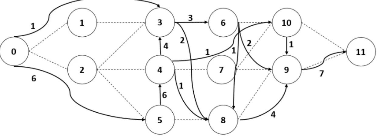
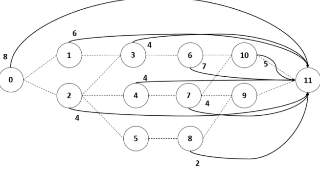
Based on the discussed MILP formulation for the RCPSP, it is possible to visualise resource transfers taking place in a project network. This can be done by introducing AON Flow Networks. An example AON Flow Network for a project consisting of 10 (real) activities and two dummy activities is depicted in figure 2.6. Here, 7 resource units are available for project execution and consequently, 7 resource units are initially stored in dummy start activity 0. Next, these resource units are passed trough the project network while ensuring for all activities i ∈ V that the amount of ingoing resource units equals the amount of outgoing resource units. Finally, the 7 resource units are collected by dummy end activity 11. In reality, different resource flows may arise in a project network since different types of resource units can be required by project activities.
Figure 2.6: AON Flow Network
2.5
Neighbourhood Structure
Analogous to the JSP, it can be investigated whether is is possible to arrive at good solutions by iteratively modifying resource chains. Again, attention must be paid
in determining the set of feasible modifications and consequently, guarantee moving from one feasible solution to another. As mentioned earlier, two types of modifica-tions will take place on the AON-Flow Network. In similarity with Poppenborg and Knust (2014), it is said that serial modifications define the Reverse Neighbourhood (Nreverse) and parallel modifications define the Reroute Neighbourhood (Nreroute).
2.5.1
Reverse Neighbourhood
In order to perform a reverse modification, two activities i ∈ V and j ∈ V with fijk > 0 for at least one resource k ∈ R are selected. For the same reasons as with JSP, no other directed path from activity i to activity j exists via other activities h ∈ V and activity i is no direct or indirect predecessor of activity j according to technological precedence constraints. Here, the next step will be to reverse the resource transfer fijk between activity i and activity j such that a new resource flow will arise.
It is very important to state that any resource flow modification must be supported by resource flow conservation identities which ensures that the sum of all resources coming in to (or released by) an activity i ∈ V remains unchanged after the modifi-cation has been completed. In practice, this means that when reversing a resource arc, attention have to be paid to resource transfers from and to the corresponding activities of which a resource arc is reversed. In this way resource flow conservation identities can be ensured and consequently, one is sure that a resource feasible flow is maintained. This is explained below using a simplified case, to provide some basic insights, after which a general case is introduced that holds under all circumstances.
Simplified Case
The simplified case was worked out by Fortemps and Hapke (1997). Here, an exam-ple project consists of four activities (activity x, activity i, activity j and activity y). It is assumed that only one resource group k is required to complete all four activi-ties. This resource flow is presented by figure 2.7 and here, the assumption is made that an activity x and an activity y exist such that fx,i,k > fi,j,k and fj,y,k > fi,j,k holds.
Next, if arc (i, j)k is reversed, then activity j is not longer able to transfer fj,y,k
Figure 2.7: Before Reverse Modification (1)
units to activity y since fi,j,k units are now transferred to activity i in order to sat-isfy its resource requirement. In addition to this, activity i receives fi,j,k units from activity j, so fi,j,k units less have to be transferred to activity i. These fi,j,k units can then be redirected from activity x to activity j and activity i will transfer fi,j,k units more to activity y. This redirection process is depicted in figure 2.8. As a result of this, it can be ensured that a reverse modification is supported by resource flow conservation identities.
Figure 2.8: After Reverse Modification (1)
General Case
Nevertheless in project scheduling, one activity can be part of different resource chains which results in the challenge of reversing multiple resource arcs at once. Thus, (i, j)k will be reversed on each resource chain k where fi,j,k > 0 holds and
consequently, special attention should be paid to resource flow conservation identi-ties on each particular resource chain.
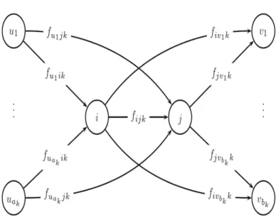
Moreover, there is no guarantee that for each resource chain k an activity x and an activity y exist, such that fx,i,k > fi,j,k and fj,y,k > fi,j,k is fulfilled. This is why, Fortemps and Hapke (1997) suggest to consider groups of predecessors or groups of successors instead of single activities. Poppenborg (2014) further elaborated on this idea and suggested the following approach.
First of all, the direction of all arcs (i, j)k for all resources k ∈ R with fijk > 0 is reversed such that fi,j,k = fj,i,k0 with fj,i,k0 = the number of resource units of resource k transferred from activity j to activity i after performing a reverse mod-ification. In addition to this, some additional resource redirecting is necessary in order to ensure resource flow conservation identities. Therefore, some extra sets and variables are introduced.
For all resources k ∈ R with fi,j,k > 0, sets Uk of activities u ∈ V0 are intro-duced. An activity u is added to Uk only if an arc (u, i)k with fuik > 0 exist. Each set Uk is expanded until the following equation holds:
X
u∈Uk
fu,i,k ≥ fi,j,k (2.10)
The size of each set Uk can be denoted by ak such that activities u1, u2, ...uak are all part of set Uk.
In addition and similar to this, for all resources k ∈ R with fi,j,k > 0, sets Vk of activities v ∈ V∗ are introduced. An activity v is added to set Vk only if an arc (j, v)k with fj,v,k > 0 exist. Each set Vk is expanded until the following equation holds:
X
v∈Vk
fj,v,k ≥ fi,j,k (2.11)
Here, the size of each set Vk can be denoted by bk such that activities v1, v2, ...vbk are all part of set Vk.
The process of selecting activities for each set Uk and Vk can be done using pri-ority rules and is discussed in section 4.1.2. Figure 2.9 (adapted from (Poppenborg and Knust, 2014) visually represents the described resource chain. Here, the groups of predecessor and successor activities have been identified.
After identifying all activities ∈ Uk and ∈ Vk, one can proceed to further modify
Figure 2.9: Before Reverse Modification (2)
resource flows such that resource flow conservation identities are ensured.
If P
u∈Ukfu,i,k > fi,j,k holds, then each set Uk can be split in one subset and one remaining activity. One subset containing all activities uλ with λ = 1, ..., ak−1 and one remaining activity, denoted as uak. Activity uak ∈ Uk corresponds to the last activity that has been selected in Uk based on the applied priority rules for defining set Uk. For all activities uλ, the resource units that originally are transferred to activity i are now redirected to activity j. This is necessary as activity j needs compensation for sending fi,j,k resource units to activity i instead of receiving fi,j,k resource units from activity i.
The subset of predecessors Uλ only partially ensure that fi,j,k resources are sent to activity j. Additionally, some extra resource units have to be sent from activity uak to activity j. These additional resource units can be calculated by the following
equation: qak = fi,j,k− ak−1 X λ=1 fuλ,i,k (2.12)
with qak representing the extra amount of resource units sent from activity uak to activity j. Hence, if P
u∈Ukfu,i,k > fi,j,k holds, it is always possible to send qak resource units from activity uak to activity j otherwise if
P
u∈Ukfu,i,k = fi,j,k holds, then no activity uak is identified and activity j is supplied by set Uk such that P
u∈Ukfu,i,k units are transferred to activity j . This is visually represented by fig-ure 2.10 (adapted from (Poppenborg and Knust, 2014).
In addition to this, fi,j,k resource units are transferred by activity j to activity Figure 2.10: After Reverse Modification (2)
i, causing a shortage of fi,j,k incoming resource units among the set of successor activities Vk. Therefore activity i will now be partially be in charge of providing these activities with the required amount of resource units.
Again, if P
v∈Vkfj,v,k > fi,j,k holds, then each set Vk can be split in one subset and one remaining activity. One subset, containing all activities vλ with λ = 1, ..., bk−1 and one remaining activity, denoted as vbk. Activity vbk ∈ Vk corresponds to the last activity that has been selected in Vk based on the applied priority rules for defining set Vk. For all activities vλ the resource units that originally were delivered by activity j are now delivered by activity i.
SinceP
v∈Vkfj,v,k > fi,j,kholds, activity i will not be able to provide enough resource units to satisfy the resource need of the whole set Vk. Therefore some resources still need to be delivered by activity j. The resource units that are delivered by activity i to activity vk can be calculated by the following equation:
qbk = fi,j,k− bk−1 X
λ=1
fuλ,i,k (2.13)
with qbk representing the extra amount of resource units sent from activity i to ac-tivity vbk. If Pv∈Vkfj,v,k = fi,j,k holds, then no activity vbk is identified and set Vk is supplied by activity j such that P
v∈Vkfv,i,k units are transferred to set Vk from activity i. This is visually represented by figure 2.10 (adapted from Poppenborg and Knust, 2014).
2.5.2
Reroute Neighbourhood
As already described, another type of modifications, namely reroute modifications, exist. Moreover, reroute modifications do not modify the activity sequence on re-source chains but allow for a different rere-source plan i.e. the way in which rere-source units are passed trough the network in order to satisfy resource requirements. This is a remarkable difference with the JSP, where the relevant machine resource is unique.
Here, two arcs (i, j)k and (u, v)k are selected such that no directed path exists from activity v to activity i and no directed path exists from activity j to activity u with fi,j,k > 0 and fu,v,k > 0 with i, u ∈ V0 and j, v ∈ V∗. This extra condition for selecting arcs is imposed such that the introduction of cycles is avoided. A more detailed explanation and practical method for this is worked out in section 3.12. The visually representation of a reroute modification is given by figure 2.11.
Then, an amount of q ∈ (1, ..., min{fi,y,k, fx,j,k}) units of resource k is redirected from activity i to activity y and an amount of q units of resource k is redirected from activity x to activity j. Figure 2.12 shows the resulting resource chain after
the modification has been completed.
Figure 2.11: Before Reroute Modification
A Practical Approach for Resource
Flow Based Project Scheduling
In Chapter 2, theoretical insights were given on how a resource flow based method can be applied to solve the RCPSP. It has been pointed out that once an initial feasible resource flow is generated, it is possible to iteratively modify this resource flow while ensuring resource flow feasibility. The purpose of repeatedly modifying resource flows is to arrive at high quality solutions.
Next, the aim of chapter 3 is to describe how previous theoretical insights can be incorporated into a practical method. Therefore, a Java project has been developed and will be used to analyse the strengths and weaknesses of this resource flow based project scheduling method.
In Chapter 3 only the methodology will be clarified, after which different design options and their impact will be discussed in more detail in Chapter 4.
3.1
Methodology
The applied methodology can be divided into three major parts, which in turn consist of several steps. The three major methodology parts are the following and will be further clarified below:
2. Solution Modification Process 3. Heuristics
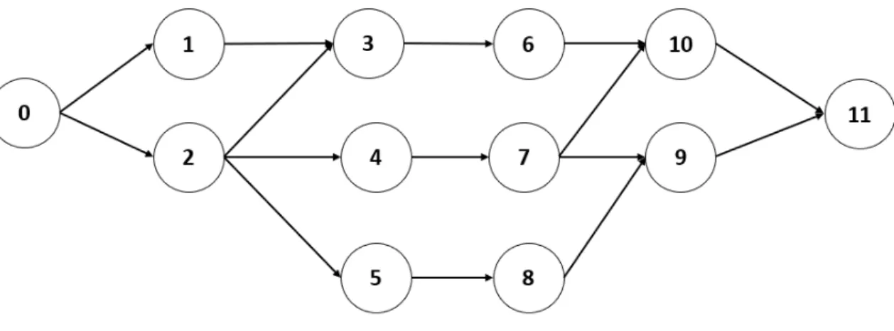
In order to facilitate the understanding of the methodology, a fictitious project case will be elaborated and serves as example to the reader for the application of several introduced techniques. The case study refers to a project consisting of ten activities.
An overview of the project activities (activity 1 → 10) and the dummy start (activity 0) and dummy end (activity 11) can be found in table 3.1 while the corresponding network diagram is presented by figure 3.1. In addition to this, two different renew-able resource types are required to process the activities. The resource availabilities are presented in table 3.2.
Example Case
Activities Duration Resource 1 Resource 2 Successors
Activity 0 0 0 0 1, 2 Activity 1 3 6 0 3 Activity 2 4 4 0 3, 4, 5 Activity 3 3 4 5 6 Activity 4 6 4 6 7 Activity 5 2 0 6 8 Activity 6 1 7 3 10 Activity 7 4 4 0 9, 10 Activity 8 5 2 4 9 Activity 9 2 0 7 11 Activity 10 3 5 1 11 Activity 11 0 0 0
-Table 3.1: Case Study: Project Overview
Resources Availabilities
Resource 1 8
Resource 2 7
Table 3.2: Case Study: Resource Availabilities
Figure 3.1: Case Study: Network diagram
phase. For now, these design options are not discussed in greater depth and are, while solving the case study, chosen without considering what options could be more appropriate. In this section the focus is on making the reader familiar with resource flow based scheduling concepts. Although, it will here be indicated wherever dif-ferent design options exist. Evaluating these difdif-ferent design options is subject of section 4.1.
3.1.1
Initial Solution Generation
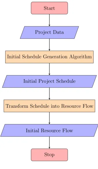
The algorithm starts with generating an initial feasible resource flow. This can be done following a two step approach. First, an initial feasible schedule is generated and is consequently transformed into a feasible resource flow. An overview of this ’Initial Solution Generation’ process is depicted by the flowchart in figure 3.3. Here and for the remainder of this thesis study, the flow chart notation of figure 3.2 is used.
Figure 3.2: Flowchart Symbols
Start/Stop Input/Output
Process Decision
Figure 3.3: Initial Solution Generation Process
Start
Project Data
Initial Schedule Generation Algorithm
Initial Project Schedule
Transform Schedule into Resource Flow
Initial Resource Flow
Stop
As the flow chart (figure 3.3) makes clear, the project data will be used as input for generating an initial schedule that does not violate any precedence or resource constraint. The output of the first step, an initial feasible schedule, will then be used as input for the second step where the initial schedule is transformed into a
feasible resource flow. Below, it is described which techniques can be applied for these two described processes.
Initial Schedule Generation
In order to determine an initial feasible schedule, several techniques can be applied. One approach is by making use of priority rule based scheduling. This technique was already mentioned as popular solution approach in section 1.3, without going into detail there. Priority rule based scheduling is in essence a quick heuristic scheduling technique that consists of two components (Vanhoucke, 2012).
The first component is a priority rule (PR) that is applied to order all project’s activities. The result of this, is an ordered activity list indicating which activities should be scheduled first and which activities should be delayed. Commonly used priority rules are the following: shortest processing time (SPT), longest processing time (LPT), most immediate successors (MIS), most total successors (MTS), earliest start time (EST), latest start times (LST), greatest work content (GWC), greatest cumulative work content (GCUMWC),... but many others exist (Vanhoucke, 2018). For the sake of simplicity, the activity numbers displayed in table 3.1 are used as priority rule in solving the case study.
The second component of priority rules based scheduling refers to a schedule genera-tion scheme. A schedule generagenera-tion scheme indicates how to extend a partial sched-ule in a stage-wise fashion (Vanhoucke, 2018). The term partial schedsched-ule refers to a schedule where only a subset of activities has been assigned a start- and finishing time.
In literature (Vanhoucke, 2011), the distinction is made between a serial sched-ule generation scheme and a parallel schedsched-ule generation scheme.
generating an initial project schedule, it is opted to only continue working with the parallel schedule generation scheme since this method is most often used in scientific literature (Poppenborg and Knust, 2014). The serial schedule generation scheme is only briefly explained by way of introduction to the parallel schedule generation scheme which is slightly different.
A serial schedule generation scheme performs an activity-incrementation and sched-ules at each stage the first activity of the priority list as early as possible without violating both the precedence constraints and the resource constraints. Once an activity is scheduled, it can be removed from the priority list such that each activity is scheduled once.
Alternatively, a parallel schedule generation scheme performs a time-incrementation rather than an activity-incrementation. Here, at each decision point t all eligible activities will be identified and consequently, eligible activities will be scheduled as long as sufficient resources are available. The order in which activities are con-sidered to be added to the partial schedule is based on the applied priority rule. The pseudocode of a parallel schedule generation scheme is displayed in algorithm 1 (adapted from (Poppenborg and Knust, 2014)) and is explained in more detail below.
Here, for each iteration λ an activity j is chosen out of the set of eligible activi-ties Eλ according to a predefined priority rule. All activities i ∈ V that can be scheduled without violating technological precedence constraints and resource con-straints are included in set Eλ. In other words, an activity i ∈ V is included in set Eλ if and only if all of its technological predecessors have been scheduled and enough resources are available to schedule activity i, i.e. rik ≤ Rk(τ ) for k = 1, ..., r with Rk(τ ) = the number of available resource units of resource k at time τ with τ = [t, t+pi[ . Once activity j is scheduled, activity j is added to the set of active ac-tivities Aλand the number of available resource units Rk(τ )for k = 1, ..., r is adapted based on the resource requirements rjk of activity j by setting Rk(τ ) = Rk(τ ) − rjk for k = 1, ..., r and τ ∈ [t, t + pj[. Then, set Eλ is updated by removing all activities i with rik > Rk(τ ) for some resource k and a τ ∈ [tλ, tλ + pi[ and consequently a
next activity j ∈ Eλ is chosen to be scheduled. This process continues, until Eλ is empty. Then, the next iteration time tλ+1 is calculated by the minimal completion time of all activities in set Aλ. This procedure is repeated until all activities i ∈ V have been scheduled and can be at most n iterations long.
Algorithm 1: Parallel Schedule Generation Scheme λ := 1; t1:=0; A1 = ∅
Let E1 be the set of all activities i without predecessor and rik ≤ Rk(τ ) for k = 1, ..., r and all τ ∈ [0, pi[
while not all activities are scheduled do while Eλ 6= ∅ do
Choose an activity j ∈ E
Schedule j in the interval [Sj, Cj[=[tλ, tλ+ pj[
Update the current resource profiles by setting Rk(τ ) := Rk(τ ) − rjk for k = 1, ..., r and τ ∈ [t, t + pj[
add activity j to Aλ
Update the set Eλ by eliminating j and all activities i with rik > Rk(τ ) for some resource k and a τ ∈ [tλ, tλ + pi[
Let tλ+1 = min{Si+ pi} be the minimal completion time of all active activities
λ := λ + 1
Calculate the new sets Aλ and Eλ
Case Study: Generating Initial Feasible Schedule
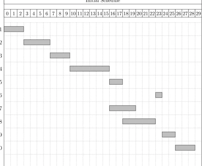
Below, the outcome of applying algorithm 1 is represented by the Gantt Chart in figure 3.4. The initial solution has a makespan of 29 time units.
Initial Flow Generation
As this thesis study focuses on resource flows and its modifications, the next step is to transform the initial schedule into a feasible resource flow. Literature (Poppenborg and Knust, 2014) has pointed out that for every feasible schedule a corresponding
Figure 3.4: Gantt Chart: Initial Project Schedule Initial Schedule 0 1 2 3 4 5 6 7 8 9 10 11 12 13 14 15 16 17 18 19 20 21 22 23 24 25 26 27 28 29 1 2 3 4 5 6 7 8 9 10
feasible resource flow can be generated. Moreover, it can be the case that for one feasible schedule, multiple feasible resource flows exist. Nevertheless, for every fea-sible resource flow only one corresponding feafea-sible earliest start schedule exist. An earliest start schedule refers to a schedule where all activities are assigned a start-ing and a finishstart-ing time as early as possible without violatstart-ing both the precedence constraints and the resource constraints.
In order to transform a feasible schedule into a feasible resource flow an adapted version of Artigues algorithm (Artigues, Demassey, and N´eron, 2010) can be ap-plied. The adaptation is implemented as it has been demonstrated that the original algorithm as proposed by Artigues is not able to transform every schedule into a feasible resource flow (Poppenborg and Knust, 2014). Since there is only a very small difference between the original algorithm and the adapted version as proposed by Poppenborg, it was decided to only discuss the latter. The pseudocode of Pop-penborg’s algorithm is presented by algorithm 2 (adapted from (Poppenborg and Knust, 2014)) and is further clarified below.
The general idea is that all outgoing resource transfers from all activities i ∈ V0 are first transferred towards the dummy end node n + 1 such that fi,n+1,k=rik for all activities i ∈ V0. The AON Flow Network presented in figure 3.5 shows the application of this first step to the case study for resource chain 1.
Thereafter, through an iterative procedure, each resource transfer will be redi-rected so that every activity i ∈ V has its resource requirement rik satisfied for all k ∈ R. During the resource redirecting process, it is tracked by variable Bik how many units of resource k ∈ R are still required by activity i ∈ V in order to be processed.
To ensure that only feasible resource transfers take place, two different activity lists (LC and LS) are generated. List LC stores all activities i ∈ V
0 according to their completion time Ci. Activities with the lowest completion times, as calculated by algorithm 1, are stored first. List LS stores all activities i ∈ V according to their
Figure 3.5: Case Study: Initial resource flow generation (1)
starting time Si. Again, activities with the lowest starting times, as calculated by algorithm 1, are stored first. Note the slight difference between activities included in list LC and activities included in list LS. The latter does not contain dummy start node 0, while the former does.
Now, it is possible to select for each activity j ∈ LS an activity i ∈ LC such that Ci ≤ Sj with i 6= j. This condition needs to be satisfied as resources can only be transferred from a completed activity i to a not yet started activity j. Next, it should be verified how many resource units of type k ∈ R are still required by activity j and how many resource units of type k are still available at activity i to be redirected towards activity j. By comparing variable Bjk and variable fi,n+1,k, the algorithm decides upon how many resource units of type k should be redirected. Hence, σ resource units = min{Bjk, fi,n+1,k} of type k are redirected from activity i to activity j. After redirecting σ units, variable Bjk and fi,n+1,k are updated and a next activity is selected from list LS. This procedure is repeated for all activities j ∈ V .
Algorithm 2: Generate resource flow from schedule Set Bik := rik for all i ∈ V and k ∈ R
Set fi,n+1,k:= rik for all i ∈ V0 and k ∈ R for j:=LS 1 to LSn do for i:=LC0 to LCn do if i 6= j then for k := R1 to Rr do if Ci ≤ Sj then σ := min {fi,n+1, Bjk} Bjk := Bjk− σ fi,n+1,k := fi,n+1,k− σ fijk := fijk+ σ
Case Study: Generating Initial Resource Flow
In order to redirect all resource transfers on resource chain 1 of the introduced case study, list Lc and list Ls are first generated. Based on the initial schedule represented by figure 3.4, list Lc={ 0, 1, 2, 3, 4, 5, 7, 8, 6, 9, 10} and Ls ={ 1, 2, 3, 4, 5, 7, 8, 6, 9, 10} are determined. If several activities should have the same starting time or the same completion time priority rules can be used as tiebreakers.
Then, the redirecting process starts by selecting the first elements in Ls and in Lc. The first element in Ls is activity 1 and the first element in Lc is activity 0. In figure 3.5, 8 resource units are initially transferred from activity 0 to dummy end activity n + 1 i.e. f0,11,1 = 8, while the resource requirement of activity 1 is equal to 6 resource units of resource type 1 i.e. B1,1 = 6. Hence, min{6, 8} units are redirected from activity 0 to activity 1 i.e. σ = 6. Now, the resource requirement of activity 1 for resource type 1 is satisfied and 2 (= 8−6) resource units are still trans-ferred from activity 0 to dummy end activity 11. This is demonstrated by figure 3.6.
Next, the second iteration starts with the selection of the second element in Ls i.e. activity 2 with B2,1 = 4. Again, the first element in Lc is considered first and now, f0,11,1 = 2. Hence, min{4, 2} resource units are redirected from activity 0 to
Figure 3.6: Case Study: Initial resource flow generation (2)
activity 2 i.e. σ = 2. As B2,1 − σ = 2, there are still 2 resource units of type 1 needed in order to satisfy the resource requirement of activity 2. Consequently, the second element in Lc is considered, which is activity 1. At activity 1, there are 6 resource units of type 1 available for redirection i.e. f1,11,1 = 6. Hence, min{2, 6} resource units are redirected from activity 1 to activity 2 i.e. σ = 2. This results in 4 resource units that are still transferred from activity 1 to dummy end activity 11 i.e. f1,11,1 = 4. This is demonstrated by figure 3.7.
Furthermore, figure 3.8 and figure 3.9 show the explicit redirecting process for activity 3 and activity 4 and the results of the complete redirecting processes for all activities i ∈ V are presented by figure 3.10 and figure 3.11 for resource flow 1 and resource flow 2 respectively.
Moreover, it has been proven by Poppenborg (2014) that this approach is able to generate a feasible resource flow for every feasible project schedule.
Figure 3.7: Case Study: Initial resource flow generation (3)
Figure 3.8: Case Study: Initial resource flow generation (4)
3.1.2
Solution Modification Process
Once an initial feasible solution has been generated, the focus is shifted to finding neighbouring solutions. For that objective, neighbourhood Nreroute and neighbour-hood Nreversewill be explored. In chapter 2 it was already investigated how a feasible resource flow can be modified while guaranteeing resource flow conservation identi-ties. This section continues on these insights and will be describe a practical method to avoid the introduction of cycles while reversing and rerouting resource arcs.
Figure 3.9: Case Study: Initial resource flow generation (5)
Figure 3.10: Case Study: Complete Initial Resource Flow (Resource 1)
After a resource flow modification is made, the next step is to assess the desir-ability of the modified resource flow is in terms of project duration. Therefore a modified resource flow must be converted into a schedule which entails assigning all activities ∈ V a start and a completion time. This can be done following a two step approach. First, the time distance between each activity i ∈ Vall and each activity j ∈ Vall will be determined. The term time distance refers to the minimal time interval that elapses between two activities. In the second step, the distance matrix
Figure 3.11: Case Study: Complete Initial Resource Flow (Resource 2)
will be applied to identify a longest path from start to end. The resulting length of that path is equal to the project’s makespan. An overview of this ’Solution Modifica-tion Process’ is depicted by the flowchart in figure 3.12 and is further clarified below.
Reverse Modification
In order to tackle the challenge of avoiding cycles while reversing resource arcs, in-spiration can be gained from the simpler JSP problem. For the JSP it was proven by Van Laarhoven (1992) that reversing critical arcs is always safe with regard to the possible introduction of cycles. Poppenborg (2014) extended this way of thinking and proved that reversing critical arcs is also safe with regard to the introduction of cycles in the RCPSP.
In this thesis study it is chosen to adopt this approach and consequently, a neigh-borhood reduction is implemented. Hence from now on, the focus will be only on reversing critical arcs. Some additional reasoning and consequences of this neigh-bourhood reduction are further discussed in section 4.1. In similarity with Poppen-borg (2014), this reduced neighbourhood is referred to as Neighbourhood Nreverseca .
Figure 3.12: Solution Modification Process
Start
Feasible Resource Flow
Select Modification Type
Reverse Modification Reroute Modification
Modified Resource Flow
Calculate Time Distances
Distance Matrix
Calculate Longest Paths
Modified Project Schedule
stop
identify them in the AON Flow Network. With this objective in mind, all critical activities will first be identified and then, it will be verified which resource
trans-fers between a pair of critical activities is critical. Additional verification whether a resource transfer is critical between a pair of critical activities is necessary as the following example demonstrate that non critical resource transfers can take place between critical activities and reversing them has the potential of introducing cycles in the AON Flow Network.
Assume a project where activity 1, 2 and 3 are critical and two types of resource transfers take place (resource A and resource B transfers). The corresponding re-source flow is depicted in figure 3.13. Now, when rere-source transfer B is reversed, a cycle is introduced and consequently, the modified solution is infeasible. This is why, the proposed two-step approach is used to identify all possible arcs that can always be safely reversed. A practical method for generating all critical activities in an AON Flow Network is presented by algorithm 3 and is further clarified below.
An activity i is critical if and only if the activity float equals zero i.e. LFi -Figure 3.13: Non critical resource transfer between a pair of critical activities
EFi = 0. Since the decision is made to schedule all activities as early as possible in this thesis study, the EFi of each activity i can be retrieved from the project schedule. Until now, nothing was tracked regarding to LFi of each activity i ∈ Vall. Therefore, all latest finish times should be calculated first.
For this objective, all activities j ∈ V0 are given a latest finishing time that is equal to the starting time of dummy end activity n + 1. This serves as an upper bound for the latest possible finishing time for all activities j ∈ V0. Then via an iterative backward procedure the latest finishing time of each activity j is adapted
depending on whether the starting time of activity i depends on the completion time of activity j. By dependent it is meant that either a technological precedence relationship or a resource transfer takes place from activity i to activity j. If this is the case, then the latest finishing time of activity j is set equal to the latest starting time of activity i.
To ensure that the correct latest finishing times are passed, the activities will first be ordered according to earliest finishing time in list LEF. Here, activities with the largest earliest finishing times are positioned first such that dependent activities are first able to pass the correct latest starting times as latest finishing times to their technological or resource predecessors.
Algorithm 3: Generate critical activities Set LFj = Sn+1 for all j ∈ V0
for i := LEF0 to LEFn+1 do LSi = LFi− pi for j := V0 to Vn+1 do if (j, i) ∈ A and LSi < LFj) then LFj = LSi for k := R1 to Rr do
if (fj,i,k > 0 and LSi < LFj)) then LFj = LSi
for i := V0 to Vn+1 do if LFi = EFi then
activity i is critical return all critical activities
After all critical activities have been determined, it can be verified which resource transfers between each pair of critical activities are critical. For this objective, al-gorithm 4 can be applied and is clarified below.
From the set of all resource arcs, it is verified which arc (i, j) consist out of both critical activities and which resource transfers can not be delayed without impacting the starting time of the receiving activity. Therefore, it is examined when a resource unit is transferred (= EFi) by activity i and when a resource unit is required (=