Limiting global temperature
change to 1.5 °C
Implications for carbon budgets, emission pathways,
and energy transitions
Note
Detlef van Vuuren, Andries Hof, David Gernaat, Harmen Sytze
de Boer
Limiting global temperature change to 1.5 °C: Implications for carbon budgets and negative emissions
© PBL Netherlands Environmental Assessment Agency The Hague, 2017
PBL publication number: 2743
Corresponding author
Detlef.vanvuuren@pbl.nl
Authors
Detlef van Vuuren, Andries Hof, David Gernaat, Harmen-Sytze de Boer
Graphics
PBL Beeldredactie
Editing and production
PBL Publishers
Acknowledgements
This note was written as part of the International Climate Project of PBL. It benefited from funding of ClimateWorks, and by the UK Government, Department for Business, Energy and Industrial Strategy, as part of the Implications of global warming of 1.5 °C and 2 °C project. This publication can be downloaded from: www.pbl.nl/en. Parts of this publication may be reproduced, providing the source is stated, in the form: Van Vuuren, D.P. et al. (2017), Limiting global temperature change to 1.5 °C: Implications for carbon budgets, emission pathways, and energy transitions. PBL Netherlands Environmental Assessment Agency, The Hague.
PBL Netherlands Environmental Assessment Agency is the national institute for strategic policy analysis in the fields of the environment, nature and spatial planning. We contribute to improving the quality of political and administrative decision-making by conducting outlook studies, analyses and evaluations in which an integrated approach is considered paramount. Policy relevance is the prime concern in all of our studies. We conduct solicited and
Findings
Emission reduction targets and carbon budgets for meeting the 1.5 and 2 °C climate targets are still uncertain, influenced by both scientific uncertainty and policy choices. There are several important factors that influence the size of the carbon budgets or medium-term emission reduction targets that are consistent with the ambition ‘to limit global temperature increase to well below 2 °C above pre-industrial levels, and to pursue efforts to limit this increase even further to 1.5 °C’. Some of them are scientific uncertainties (e.g. limitations in the understanding of the climate system), but others are policy choices (the level of overshoot allowed in reaching the targets; the probability with which the target should be achieved).
Under all assumptions and policy choices, the Paris Climate Agreement requires very stringent emission reductions. Emission scenarios using global models show that very stringent emission reductions are needed if cumulative CO2
emissions need to be restricted to 1000 GtCO2, or significantly less, in the
remainder of the century.
Scenarios show that, technology-wise, pathways that can reach the
climate goals still exist. There are different pathways towards achieving the Paris Climate targets. These scenarios assume that it is possible to implement climate policies in most regions, leading to a peak in global emissions within the next decade, followed by rapid reductions.
Most 1.5 and 2 °C scenarios show the use of negative CO2 emission
technologies. At the same time, in reality only relatively small investments are made in these technologies, and people have raised concerns regarding large-scale use. In order to compensate emission sources that are very difficult to mitigate, and to allow limited overshoot of the carbon budgets in the short term, model-based scenarios show extensive use of negative emission technologies. As, currently, the support for these technologies is low and experience in large-scale application is lacking, it is important to discuss the feasibility of these pathways, more explicitly.
The reliance of negative emissions from bio-energy can be reduced. However, broadening the portfolio of options that are considered and/or deeper reductions in other options are required. Lifestyle change, including changes in diet patterns and using less energy-intensive transport modes, can reduce emissions but are not often included in mitigation studies. Moreover, it is possible to consider more intensive use of other options such as deeper reduction of non-CO2 emissions, or promoting more reforestation.
1 Introduction
Under the Paris Climate Agreement (December 2015), nearly all countries in the world, including the Netherlands, agreed to limit global temperature increase to well below 2 °C above pre-industrial levels, and to pursue efforts to limit this increase even further to 1.5 °C (UNFCCC, 2015). Scenario literature shows that achieving these objectives requires deep reductions in greenhouse gas emissions. However, the exact ambition level depends on several factors not specified in the agreement itself, notably the role of timing, probability to achieve the climate goals, risk thresholds, temporary overshoot, negative emissions, and the ability to make decisions in the context of these uncertainties and policy decisions. At the moment, the Paris Climate Agreement does not specify these dimensions. While leaving concepts somewhat ambiguous is often intentional in climate negotiations, it will be necessary to translate the overall objective of the Paris Climate Agreement into very concrete mitigation targets at all relevant scales to support effective negotiations. The scientific community can add value by providing the information necessary to identify, understand, interpret and, eventually, resolve these
ambiguities. In this publication, we briefly explore the implications of the 1.5 °C target according to different assumptions regarding the above uncertainties and decisions on carbon budgets (Section 2), and on emission pathways and energy system implications (Section 3).
2 Carbon budgets
consistent with 1.5 °C
2.1 Important consideration for defining the 1.5 °C target
The Paris Climate Agreement’s main objective is to limit the increase in global mean temperature to well below 2 °C, and to pursue efforts to limit it to 1.5 °C (UNFCCC, 2015). There are several aspects that need to be considered to understand what these targets imply for required reductions in CO2 emissions:• Time dimension: How to deal with a temporary overshoot? If an overshoot is allowed, when should the target be achieved?
• Probability dimension: With what likelihood should the target be achieved? • Contribution of various gases and forcing agents: There are various gases
and other forcing agents contributing to climate change. How will the forcing for each of them develop over time?
• Reference point: What is the reference warming? And the current level of warming?
There is no single, definitive answer to the questions related to these dimensions, and approaches differ between researchers and disciplines. These questions are already important for the 2 °C climate target, but even more so for more stringent targets.
The importance of different interpretations of the 1.5 °C target can be illustrated using information from scientific publications as well as from the IPCC’s Fifth Assessment Report (AR5) Working Group III database (Clarke et al., 2014; Krey et al., 2014). For all scenarios for which sufficient information was available, climate change implications were calculated using the simple climate model MAGICC (Meinshausen et al., 2011). In the IPCC database, seven categories of scenarios were defined, based on their level of climate change (expressed as radiative forcing levels in 2100) (Figure 2.1). The lowest of these categories leads to forcing levels around 2.6 W/m2, which is the lowest Representative Concentration Pathway (RCP)
scenario (Van Vuuren et al., 2011) run by complex climate models in preparation of the last IPCC report.
The figure shows the median value for each category in the IPCC AR5 WGIII scenario database for CO2
emissions (panel a), the increase in global mean temperature (panel b) and the probability of staying below 1.5 °C (panel c) for all scenarios included in the AR5 WGIII Scenario database (Clarke et al., 2014; Krey et al., 2014).
Time dimension
Time plays a role, as many scenarios that meet stringent climate targets include some degree of overshoot of the maximum allowed level of cumulative greenhouse gas emissions and sometimes even the temperature target (Figure 2.1). To
illustrate this, the median value for temperature in the two lowest categories (middle panel) peaks mid century, despite rapidly declining emission levels (left panel). As a result, the median scenario in the lowest scenario category in the AR5 WG III database has about a 20% chance to stay below 1.5 °C throughout the century (given the uncertainty in the climate system), but a 35% by the end of the century (right panel). Allowing overshoot provides some more flexibility in
achieving the 1.5 °C target, but has the disadvantage of increasing the risk of triggering tipping-point impacts that are difficult to reverse, such as those
associated with melting of permafrost areas or the Greenland ice cover (these are not included in the calculations). Timing also has implications for the types of technologies that need to be deployed in order to achieve the target. For instance, higher levels of overshoot imply a greater dependence on carbon dioxide removal (CDR) technologies to compensate for the overshoot.
Probability dimension
The probability dimension, here, concerns the level of confidence about an emission pathway achieving a certain temperature target. Impacts of climate change are a function of local changes in temperature, precipitation and other variables. Research suggests that these variables correlate with the average global mean warming level. However, uncertainty in the climate change system implies that we do not know precisely how climate change aligns with greenhouse gas
concentration levels. This uncertainty is captured in the common practice of referring to a scenario in terms of the probability that warming will stay below a certain level. Scientific literature, often, uses likely chance (>66%) (e.g.
Meinshausen et al., 2006; Rogelj et al., 2016a), but other probabilities are used, as well. The implication is that RCP 2.6 is often considered a 2 °C scenario in
approaches that consider climate uncertainty (based on the 66% probability), but can be – and is – used as a 1.5 °C scenario in approaches that do not, as the mean warming of this pathway is 1.6 °C over the 2081–2100 period (IPCC, 2013) (Figure 2.1, middle panel).
Contribution of different gases
There are a number of factors that contribute to anthropogenic global warming. CO2
forcing constitutes the most important greenhouse gas, but methane (CH4), nitrous
oxide (N2O) and various halogenated gases (CFCs, HFCs, PFCs, SF6) also contribute
to the increase in greenhouse gases in the atmosphere. Furthermore, changes in land cover can contribute to climate change, most importantly via a change in the earth’s albedo; for instance, driven by expansion of agricultural area or
reforestation. All climate forcers have different characteristics in terms of their lifetime and contribution to climate change. Although there are metrics to translate these contributions into CO2-equivalent emissions and concentration levels, the
relationship between CO2 emissions and climate change depends on the
development of each forcing agent, over time.
Reference temperature
The Paris Climate Agreement defines the objective for the increase in global mean temperature relative to pre-industrial levels. There are a number of questions related to the definition of ‘pre-industrial levels’ and the measurement of the global mean temperature (how to average different measurements, and the time period to be averaged). The IPCC’s AR5 report uses the 1850–1900 period as the period to calculate the reference temperature. The use of this time period is not undisputed, as there were some large volcanic eruptions, and greenhouse gas concentrations had already started to increase (Schurer et al., 2017). Alternative time periods have been proposed, including 1861–1880 (a period without major volcanic eruptions, but with a temperature comparable to that of the 1850–1900 period), and 1720–1800 (as a period without anthropogenic warming). The differing data sets used for measuring temperature and the differing methods to interpret these data can also result in considerable uncertainty. On the basis of a statistical method to estimate across several data sets, with 1880 taken as the base year, global average temperature change would be 1.01 ± 0.13 °C over the period up to 2016 (Visser et al., 2017).
2.2 Carbon budgets for the 1.5 °C target
In recent scientific literature, the implications of long-term temperature targets are often expressed in terms of so-called carbon budgets, i.e. the total amount of carbon dioxide (CO2) emissions, over time. This expression is a slight simplification,
as it ignores the contribution of other greenhouse gases, but has the advantage of emphasising that climate change depends not so much on emissions in a target year (e.g. 2050) but rather on total emissions, over time, including those in the short term.
The relationship between cumulative CO2 emissions and temperature change can be used for deriving a
global carbon emissions budget that is consistent with the objectives of the Paris Climate Agreement. The coloured plane represents the range of results from climate models and, therefore, is indicative of the degree of uncertainty. The plane also shows the median and the 67th percentile. The circles depict the various scenario categories, as used in the recent IPCC report, on the basis of CO2 equivalent
concentrations. The size of the circles is determined, among other things, by the uncertainty about non-CO2 emissions.
In its AR5 report, IPCC in fact emphasised the relationship between long-term temperature levels and cumulative CO2 emissions (Figure 2.2) (Friedlingstein et al.,
2014; IPCC, 2014; Meinshausen et al., 2009; Rogelj et al., 2016b). This relationship between temperature and CO2 means that carbon budgets can be
determined for various climate targets. However, the points made in Section 2.1 obviously come up — and, sometimes pragmatic, decisions need to be made. The coloured plane of Figure 2.2 shows the range resulting from a large number of climate models, indicating the uncertainty related to the limited knowledge about the climate system (as indicated in the second issue in Section 2.1). Because of this uncertainty, a given temperature level (y-axis) corresponds with a range of values of the carbon emissions budget (x-axis). Figure 2.2 may also be used to derive the probability of achieving a certain climate target for a given emissions budget. Points along the median line indicate that the budget on the x-axis leads to about a 50% likelihood of staying below the temperature value on the y-axis. For each point above this line, the same carbon emissions budget provides a greater likelihood of staying below the related temperature level (y-axis). The second line in the figure
shows the points at which the related temperature target could be achieved with a 66% likelihood. This value is termed likely in IPCC uncertainty definitions (second issue raised in Section 2.1).
The impact of the uncertainty in non-CO2 emissions (third item in Section 2.1) on
the carbon budget is represented by the circles in Figure 2.2; because of uncertainty about non-CO2 emissions, the various values of the CO2 emissions
budget within each circle may result in a comparable temperature change. The impact is somewhat smaller than that of the uncertainty in the climate system. The aspect timing and overshoot comes back in the various methods that are used in the literature for deriving carbon budget values. Rogelj et al. (2016b) make a distinction between threshold exceedance budgets (TEB) and threshold avoidance budgets (TAB). The exceedance budget is defined as the cumulative level of CO2
emissions until a specified temperature is reached. In Figure 2.2, the exceedance budgets can be found simply by reading the budget related to a temperature change level. The second method is based on the results of Integrated Assessment Models and equals the total cumulative CO2 emissions in mitigation scenarios that
just avoid exceeding the temperature target. Simply based on the calculation method, TAB leads to lower estimates of the carbon budget (the approach requires the temperature increase to slow down to zero before the temperature target is reached). However, most applications of the TEB method also assumes higher non-CO2 emissions, as they are based on a non-mitigation scenario, thereby cancelling
some of this effect.
Rogelj et al. (2016b) provides a whole range of carbon budget estimates published before 2016, taking into account the various uncertainties. For a more than 66% likelihood of achieving the 2 °C target, they suggest that the carbon budget from 2015 onwards must range from about 600 to 1200 GtCO2 (mostly depending on
assumptions regarding non-CO2 emissions). This equals around 15 to 30 years of
current annual emissions (Le Quéré et al., 2015). Reported budgets for 1.5 °C in the IPCC Synthesis Report are around 400 GtCO2 and 240 GtCO2 based on a
respective 50% and 66% of the simulations meeting the 1.5 °C target (IPCC, 2014), or 10 and 5 years of current annual emissions. Table 2.1 provides an overview of the values from the IPCC report (IPCC, 2014).
A recent paper by Millar et al. (2017) provides considerably higher numbers than the IPCC and Rogelj et al (2016b). One important reason is that Millar et al. re-estimated the IPCC’s figures (as shown in Figure 2.2) on the relationship between the cumulative CO2 emissions and long-term warming by looking at warming and
budget from the present day onwards, instead of the earlier practice of looking at longer term trends and, subsequently, correcting for historical emissions. The Millar method is less influenced by possible bias in warming in climate models in the historic period, but it requires an estimation of current warming in order to define the still allowable warming from 2015 onwards. Millar et al. used a value for present day warming of 0.93 °C compared to pre-industrial, which is in the lower range of estimates of historic warming (leading to a higher budget for remaining emissions). The budgets published by Millar et al. are 730–880 GtCO2 for a 1.5 °C
target, and around 1400 GtCO2 for a 2 °C target, both with at least 66%
probability. Using the median estimate of historic warming from Visser et al. (see Section 2.1) would reduce the Millar et al. budgets to 600–680 GtCO2 for 1.5 °C,
and to 1300 GtCO2 for 2 °C. Millar et al. also improved the TEB method in
difference with the estimates by Rogelj et al. (2016b) and the IPCC can be
understood in terms of the use of exceedance versus avoidance numbers (as can be deducted from comparing the exceedance and avoidance numbers reported by Rogelj et al. (2016b)).
Table 2.1: Overview of the carbon emissions budget from 2015 onwards for achieving different temperature targets at different probabilities (GtCO2)
Likelihood of staying below 1.5 °C Likelihood of staying below 2 °C
At least 50% At least 66% At least 50% At least 66% 390–440 240 (no range
available) 1140 (990–1240) 840 (590–1240) Source: IPCC, 2014a (values have been corrected for emissions over the 2011–2014 period)
Overall, it can be concluded that the exact carbon budget for the ‘1.5 °C’ target depends on scientific uncertainty and on the likelihood at which the target should be achieved. However, in all cases, the budget will be very stringent.
3 Emission and energy
scenarios consistent
with the 1.5 °C target
3.1 Emission pathways
Climate models can be used to design scenarios that achieve long-term climate targets at certain probabilities. This chapter explores the implications of various carbon budgets for emission pathways.
Box 3.1: IMAGE-model-based scenarios
The analysis presented here used the integrated assessment model IMAGE (Stehfest et al., 2014) to explore alternative pathways leading to a radiative forcing level of 1.9 W/m2 by
2100. The IMAGE model can assess the implications of various mitigation strategies, in terms of changes in energy systems, land use, emissions and associated costs. The scenarios analysed here are all based on the IMAGE implementation of the SSP2 scenario, which is a middle-of-the-road scenario on socio-economic developments (Van Vuuren et al., 2017). In the standard set-up of the model, extensive-mitigation scenarios are implemented via the introduction of a uniform global carbon price, resulting in a strategy similar to other scenarios in the literature (Van Vuuren et al., 2017).
Baseline and current policy
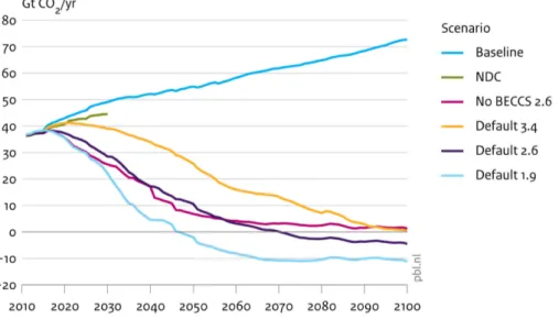
The baseline scenario shows the trajectory for CO2 emissions according to a
hypothetical scenario in which no new or additional climate policies are introduced. In this case, global CO2 emissions are projected to reach annual emission levels of
around 60 GtCO2 by 2050, and 75 GtCO2 by the end of the century. IPCC provides a
full uncertainty range of cumulative emissions of 3500–6500 GtCO2 (which is
consistent with our numbers). By 2100, this would lead to a global temperature rise of between 3 and 7 °C, compared to pre-industrial levels (Clarke et al., 2014). Implementing current climate policies formulated in many countries around the world will lead to some emission reduction as shown by the NDC scenario, but will be insufficient to achieve ambitious climate goals (Figure 3.1).
Stringent mitigation scenarios
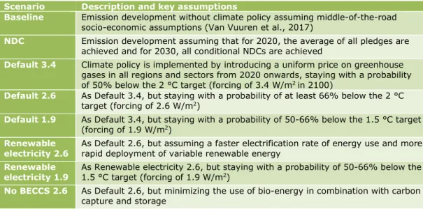
Emission reduction pathways that comply with the Paris Climate Agreement show rapid emission reductions. Figure 3.1 provides an overview of pathways that could lead to the 1.5 °C target with medium probability, and 2 °C target with medium and likely probability. The scenarios are introduced in Table 3.1.
Table 3.1: Scenarios included in this note
Scenario Description and key assumptions
Baseline Emission development without climate policy assuming middle-of-the-road socio-economic assumptions (Van Vuuren et al., 2017)
NDC Emission development assuming that for 2020, the average of all pledges are achieved and for 2030, all conditional NDCs are achieved
Default 3.4 Climate policy is implemented by introducing a uniform price on greenhouse gases in all regions and sectors from 2020 onwards, staying with a probability of 50% below the 2 °C target (forcing of 3.4 W/m2in 2100)
Default 2.6 As Default 3.4, but staying with a probability of at least 66% below the 2 °C target (forcing of 2.6 W/m2)
Default 1.9 As Default 3.4, but staying with a probability of 50-66% below the 1.5 °C target (forcing of 1.9 W/m2)
Renewable
electricity 2.6 As Default 2.6, but assuming a faster electrification rate of energy use and more rapid deployment of variable renewable energy
Renewable
electricity 1.9 As Renewable electricity 2.6, but staying with a probability of 50-66% below the 1.5 °C target (forcing of 1.9 W/m2)
No BECCS 2.6 As Default 2.6, but minimizing the use of bio-energy in combination with carbon capture and storage
In the literature, scenarios reaching 2.6 and 1.9 W/m2 are often regarded as
interpretations of the climate objectives of the Paris Climate Agreement. They correspond more or less to the 2 °C and 1.5 °C carbon budgets discussed in the previous section (as also indicated in the definitions in Table 3.1). Both scenarios show a global peak in CO2 emissions in the short term, followed by a period of rapid
reductions and, ultimately, negative CO2 emissions.
Theoretically, these targets can still be reached using pathways without negative CO2 emissions. Without negative CO2 emissions, however, scenarios cannot
temporarily exceed the carbon budgets and, therefore, even more rapid emission reductions are needed. For achieving the 1.5 °C target, CO2 emissions would need
to decline to zero in about 12-20 years (around 2025-2035), depending on the likelihood, using the carbon budget provided by the IPCC and assuming linear emission reductions. It seems unlikely that this will be feasible, given current emission trends and the lifetime of infrastructure and technologies. If net negative CO2 emissions are achieved, the year by which carbon neutrality needs to be
achieved can be delayed by about 10 to 15 years, which means that rapid reductions are still needed.
There are several methods to achieve negative CO2 emissions. The most common
CDR options in scenario analyses are reforestation and the use of bio-energy in combination with carbon capture and storage (BECCS). Other, less often, considered options include direct air capture (using carbon dioxide scrubbers to absorb the CO2 that is already in the atmosphere) and enhanced weathering. When
the amount of negative CO2 emissions is larger than the fossil-fuel emissions
remaining in the air, this is referred to as ‘net negative CO2 emissions’. Nearly all
IPCC scenarios rely on net negative CO2 emissions to achieve the 2 °C target with a
likely chance (Van Vuuren et al., 2015). Therefore, the Paris Climate Agreement implicitly relies on negative emissions as well, as the targets in the agreement are based on IPCC scenarios and underlying literature.
Across the range of scenarios, the amount of net negative CO2 emissions in 2 °C
scenarios typically varies from zero to over 350 GtCO2, for the second half of this
century (equal to up to 10 years of current annual energy- and industry-related CO2
emissions). It is important to realise that CDR technologies cannot be applied without restriction, as there are biophysical limits to afforestation, bio-energy generation and carbon storage (Smith et al., 2016). Moreover, both bio-energy generation and carbon storage are controversial methods, because of possible undesirable effects, such as on food security, biodiversity, emissions, and risks related to CO2 storage. This leads to questions about the feasibility of scenarios that
rely on large-scale storage (Anderson and Peters, 2016) —especially, since, to date, CO2 storage has hardly been applied— and about the feasibility of scenarios that do
not rely on CDR technologies. A more in-depth discussion on the pros and cons of the various mitigation strategies is urgently needed.
3.2 Energy systems
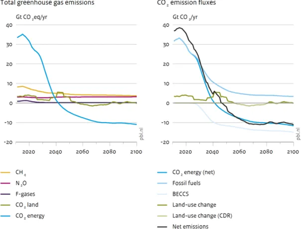
Figure 3.2 depicts a more detailed picture of the total greenhouse gas emissions (panel a) and CO2 emissions (panel b) of the Default 1.9 scenario. Both CO2 and
non-CO2 emissions are reduced, rapidly. However, despite these rapid emission
reductions in the short term, total non-CO2 emission reductions are constrained.
The main reason is that, for several sources, only a limited reduction potential has been identified (e.g. for rice cultivation and animal husbandry). For CO2, the right
panel shows how the net emissions (represented by the black line, equal to the Default 1.9 scenario in Figure 3.1) are the result of positive and negative fluxes in the energy and land-use systems. This ‘decomposition’ also shows that some fossil-fuel-related emission sources are difficult to reduce. This is especially the case for transport emissions from aviation and shipping. In addition, a certain amount of emissions remains in the atmosphere as a result of imperfect capture rates of CO2
at power plants and in industries with carbon-capture-and-storage (CCS) systems. As a result, even if CO2 emissions turn net negative, some positive
fossil-fuel-related CO2 emissions will remain in the atmosphere until the end of the century.
emissions are achieved, thereby already partly offsetting remaining CO2 emissions
from these other sources. Land-use-related CO2 emissions are projected to remain
close to zero, from 2050 onwards. This is a result of opposing trends; area
expansion for bio-energy production increases emissions due to loss of vegetation, whereas afforestation decreases emissions. The trends in the Default 2.6 scenario are similar, but somewhat slower in time.
It is possible to reduce the need for negative emissions and still achieve ambitious climate goals. Such strategies include: 1) a further decrease in non-CO2 emissions;
2) reducing the remaining CO2 emissions; and 3) including the contribution of
reforestation and afforestation (which also leads to negative CO2 emissions). Here,
we show the impact of two scenarios that limit the use of negative CO2 emissions;
one that does so by relying more heavily on further electrification (the Renewable electricity scenarios), and one that places explicit restrictions on the use of BECCS (the No BECCS scenario, which requires a considerably higher carbon price to achieve the same radiative forcing level). The results from these scenarios show that it is possible to limit the use of BECCS, but also that it is very difficult to completely avoid negative CO2 emissions, especially for 1.5 °C.
Figure 3.3 shows the cumulative contributions of all CO2 emission sources for all
scenarios in Table 3.1, retaining the colour scheme of the right panel of Figure 3.2. The total CO2 budget over the 2010–2100 period is the result of the net flow of
cumulative emissions related to energy and land use. The net total emissions vary between 2050 GtCO2 (Default 3.4 scenario) and 325 GtCO2 (Default 1.9 scenario).
Further reducing non-CO2 emissions could allow for somewhat higher cumulative
Figure 3.4 shows that, in all scenarios, the global energy system is converted from one that is based almost completely on fossil fuels (currently) to one in which renewable energy, nuclear power or CCS play an important role. Here, also, the transformation of the energy system needs to occur more rapidly in the scenario relevant for the 1.5 °C target than in the one aiming for 2 °C. This is especially visible in the faster phase-out of oil; for achieving the 1.5 °C target, not only coal, but also unmitigated oil use should be largely phased out by 2050. At the same time, bio-energy is projected to increase, both with and without CCS. Moreover, given the stringent budget in the 1.5 °C scenario, BECCS is deployed on a larger scale than in the 2 °C scenario. The use of CCS and bio-energy can be limited, substantially, in the 2 °C scenarios that explore less BECCS use (the Renewable electricity and No BECCS scenarios), but achieving 1.5 °C is extremely difficult without this technology.
References
Anderson K, Peters G. (2016). The trouble with negative emissions. Science 354:182–183.
Clarke L, Jiang K, Akimoto K, Babiker M, Blanford G, Fisher Vanden K, Hourcade J, Krey V, Kriegler E, Löschel A, McCollum D, Paltsev S, Rose S, Shukla PR, Tavoni M, Van der Zwaan B and Van Vuuren DP. (2014). Assessing Transformation Pathways. in Edenhofer O, Pichs-Madruga R, Sokona Y, Farahani E, Kadner S, Seyboth K, Adler A, Baum I, Brunner S, Eickemeier P, Kriemann B, Savolainen J, Schlömer S, von Stechow C, Zwickel T, Minx JC (eds.), Climate Change 2014: Mitigation of Climate Change. Contribution of Working Group III to the Fifth Assessment Report of the Intergovernmental Panel on Climate Change. Cambridge University Press, Cambridge (UK).
Friedlingstein P, Andrew RM, Rogelj J, Peters GP, Canadell JG, Knutti R, Luderer G, Raupach MR, Schaeffer M, Van Vuuren DP and Le Quéré C. (2014). Persistent growth of CO2 emissions and implications for reaching climate targets. Nature
Geoscience 7:709–715.
IPCC (2013). Summary for policymakers. in Stocker TF, Qin D, Plattner GK, Tignor M, Allen SK, Boschung J, Nauels A, Xia Y and Be V. (eds.), Climate Change 2013: The Physical Science Basis. Contribution of Working Group I to the Fifth Assessment Report of the Intergovernmental Panel on Climate Change.
IPCC (2014). Climate Change 2014 - Synthesis Report. Intergovernmental Panel on Climate Change.
Krey V, Masera O, Blanford G, Bruckner T, Cooke R, Fisher-Vanden K, Haberl H, Hertwich EG, Kriegler E, Mueller D, Paltsev S, Price L, Schlömer S, Ürge-Vorsatz D, Van Vuuren DP and Zwickel T. (2014). Annex II: Metrics & Methodology. in Edenhofer O, Pichs-Madruga R, Sokona Y, Farahani E, Minx JC, Kadner S,
Seyboth K, Adler A, Baum I, Brunner S, Eickemeier P, Kriemann B, Salvolainen J, Schlömer S, Stechow Cv and Zwickel T (eds.), Climate Change 2014: Mitigation of Climate Change. Contribution of Working Group III to the Fifth Assessment Report of the Intergovernmental Panel on Climate Change. Cambridge University Press, Cambridge (UK) and New York (NY).
Le Quéré C, Moriarty R, Andrew RM, Canadell JG, Sitch S, Korsbakken JI, Friedlingstein P, Peters GP, Andres RJ, Boden TA, Houghton RA, House JI, Keeling RF, Tans P, Arneth A, Bakker DCE, Barbero L, Bopp L, Chang J,
Chevallier F, Chini LP, Ciais P, Fader M, Feely RA, Gkritzalis T, Harris I, Hauck J, Ilyina T, Jain AK, Kato E, Kitidis V, Klein Goldewijk K, Koven C, Landschützer P, Lauvset SK, Lefévre N, Lenton A, Lima ID, Metzl N, Millero F, Munro DR, Murata A, Nabel J, Nakaoka S, Nojiri Y, O'Brien K, Olsen A, Ono T, Pérez FF, Pfeil B, Pierrot D, Poulter B, Rehder G, Rödenbeck C, Saito S, Schuster U, Schwinger J, Séférian R, Steinhoff T, Stocker BD, Sutton AJ, Takahashi T, Tilbrook B, van der Laan-Luijkx IT, van der Werf GR, van Heuven S, Vandemark D, Viovy N,
Wiltshire A, Zaehle S and Zeng N. (2015). Global Carbon Budget 2015. Earth System Science Data 7:349–396.
Meinshausen M, Hare B, Wigley TML, Van Vuuren D, Den Elzen MGJ and Swart R. (2006). Multi-gas emissions pathways to meet climate targets. Climatic Change 75:151–194.
Meinshausen M, Meinshausen N, Hare W, Raper SCB, Frieler K, Knutti R, Frame DJ and Allen MR. (2009). Greenhouse-gas emission targets for limiting global warming to 2°C. Nature 458:1158–1162.
Meinshausen M, Raper SCB and Wigley TML. (2011). Emulating coupled
atmosphere-ocean and carbon cycle models with a simpler model, MAGICC6: Part I - model description and calibration. Atmos. Chem. Phys. 11:1417–1456.
Millar RJ, Fuglestvedt JS, Friedlingstein P, Rogelj J, Grubb MJ, Matthews HD, Skeie RB, Forster PM, Frame DJ and Allen MR. (2017). Emission budgets and pathways consistent with limiting warming to 1.5 °C. Nature Geoscience 10:741–747. Rogelj J, Den Elzen M, Höhne N, Fransen T, Fekete H, Winkler H, Schaeffer R, Sha
F, Riahi K and Meinshausen M. (2016a). Paris Agreement climate proposals need a boost to keep warming well below 2 °C. Nature 534:631–639.
Rogelj J, Schaeffer M, Friedlingstein P, Gillett NP, Van Vuuren DP, Riahi K, Allen M and Knutti R. (2016b). Differences between carbon budget estimates unravelled. Nature Climate Change 6:245–252.
Schurer AP, Mann ME, Hawkins E, Tett SFB and Hegerl GC. (2017). Importance of the pre-industrial baseline for likelihood of exceeding Paris goals. Nature Climate Change 7:563–567.
Smith P, Davis SJ, Creutzig F, Fuss S, Minx J, Gabrielle B, Kato E, Jackson RB, Cowie A, Kriegler E, Van Vuuren DP, Rogelj J, Ciais P, Milne J, Canadell JG, McCollum D, Peters G, Andrew R, Krey V, Shrestha G, Friedlingstein P, Gasser T, Grübler A, Heidug WK, Jonas M, Jones CD, Kraxner F, Littleton E, Lowe J,
Moreira JR, Nakicenovic N, Obersteiner M, Patwardhan A, Rogner M, Rubin E, Sharifi A, Torvanger A, Yamagata Y, Edmonds J and Yongsung C. (2016). Biophysical and economic limits to negative CO2 emissions. Nature Climate
Change 6:42–50.
Stehfest E, Van Vuuren DP, Bouwman AF, Kram T, Alkemade R, Bakkenes M, Biemans H, Bouwman A, Den Elzen MGJ, Jansen J, Lucas P, Van Minnen J, Müller M. and Prins A. (2014) Integrated Assessment of Global Environmental Change with IMAGE 3.0. Model description and policy applications. PBL Netherlands Environmental Assessment Agency, The Hague.
UNFCCC (2015) FCCC/CP/2015/L.9/Rev.1: Adoption of the Paris Agreement. UNFCCC, Paris.
Van Vuuren DP, Edmonds J, Kainuma M, Riahi K, Thomson A, Hibbard K, Hurtt GC, Kram T, Krey V, Lamarque JF, Masui T, Meinshausen M, Nakicenovic N, Smith SJ and Rose SK. (2011). The representative concentration pathways: an overview. Climatic Change 109:5–31.
Van Vuuren DP, Van Sluisveld MAE and Hof AF. (2015). Implications of long-term scenarios for medium-term targets (2050). PBL Netherlands Environmental Assessment Agency, The Hague.
Van Vuuren DP, Stehfest E, Gernaat DEHJ, Doelman JC, van den Berg M, Harmsen M, de Boer HS, Bouwman LF, Daioglou V, Edelenbosch OY, Girod B, Kram T, Lassaletta L, Lucas PL, van Meijl H, Müller C, van Ruijven BJ, van der Sluis S and Tabeau A. (2017). Energy, land-use and greenhouse gas emissions trajectories under a green growth paradigm. Global Environmental Change 42:237–250. Visser H, Dangendorf S, Van Vuuren DP, Bregman B and Petersen AC. (2017).
Signal detection in global mean temperatures after “Paris”: an uncertainty and sensitivity analysis. Clim. Past Discuss doi.org/10.5194/cp-2017–88.