2 °C and 1.5 °C scenarios and possibilities of limiting the use of BECCS and bio-energy

2

°

_{C AND 1.5}

°

_{C SCENARIOS AND}

POSSIBILITIES OF LIMITING THE

USE OF BECCS AND BIO-ENERGY

Note

Kendall Esmeijer, Michel den Elzen, David Gernaat, Detlef van

Vuuren, Jonathan Doelman, Kimon Keramidas, Stéphane

Tchung-Ming, Jacques Després, Andreas Schmitz, Nicklas

Forsell, Petr Havlik and Stefan Frank

2 °C and 1.5 °C scenarios and possibilities of limiting the use of BECCS and bio-energy

© PBL Netherlands Environmental Assessment Agency The Hague, 2018

PBL publication number: 3133

Corresponding author

michel.denelzen@pbl.nl

Authors

Kendall Esmeijer, Michel den Elzen, David Gernaat, Detlef van Vuuren, Jonathan Doelman (PBL)

Kimon Keramidas, Stéphane Tchung-Ming, Jacques Després, Andreas Schmitz (JRC) Nicklas Forsell, Petr Havlik, Stefan Frank (IIASA)

Graphics

Kendall Esmeijer

Production coordination

PBL Publishers

This document has been prepared by PBL/NewClimate Institute/IIASA under contract to DG CLIMA (EC service contract No. 340201/2017/64007/SER/CLIMA.C1), started in December 2017.

This project is being funded by the EU:

This publication can be downloaded from: www.pbl.nl/en. Parts of this publication may be reproduced, providing the source is stated, in the form: Esmeijer, K. et al. (2018), 2 °C and 1.5 °C scenarios and possibilities of limiting the use of BECCS and bio-energy. PBL

Netherlands Environmental Assessment Agency, The Hague.

PBL Netherlands Environmental Assessment Agency is the national institute for strategic policy analysis in the fields of the environment, nature and spatial planning. We contribute to improving the quality of political and administrative decision-making by conducting outlook studies, analyses and evaluations in which an integrated approach is considered paramount. Policy relevance is the prime concern in all of our studies. We conduct solicited and

Contents

MAIN FINDINGS

4

1

INTRODUCTION

7

2

MODELLING SET-UP

9

General scenario formulation 12

2.3.1 IMAGE model 12

2.3.2 POLES model 14

Mitigation scenarios for meeting 1.5 °C and 2 °C targets 16

2.4.1 Model implementation of scenarios 18

3

CURRENT POLICIES AND FULL TECHNOLOGY MITIGATION

SCENARIOS

20

Current policies scenarios 20

The 2 °C Full technology scenarios 22

The 1.5 °C Full technology scenarios 27

4

ALTERNATIVE SCENARIOS

32

The 2 °C alternative scenarios 32

The 1.5 °C alternative scenarios 39

5

LAND-USE SYSTEM

44

LULUCF emissions and removals 45

Agricultural sector and non-CO2 greenhouse gases 47

Land-cover change 49

Food security 54

6

EU ANALYSIS

56

7

REFERENCES

58

Main findings

Model-based scenarios show pathways that limit global warming to well below 2 °C or further down to 1.5 °C. This report presents a range of scenarios that limit warming to

well below 2 °C and to 1.5 °C, using IMAGE (PBL) and POLES (JRC) models. More specifically, the 2 °C and 1.5 °C scenarios are consistent with limiting global warming to below 2 °C in the 21st century, and to 1.5 °C by 2100, with a respective probability of at least 66% and 50%. The results show that these targets can be achieved, technically, under

Full technology scenarios (i.e. using all available technologies). Such full technology

scenarios rely on rapid and deep emission reductions through a mix of i) energy efficiency improvements, ii) rapid introduction of energy options without CO2 emissions (e.g.

renewable energy and CCS), iii) negative emission options (e.g. bio-energy with CCS

(BECCS) and afforestation), and iv) reduction in non-CO2 gases. Under the IMAGE scenarios,

contributions of energy efficiency improvements and CCS are larger than under the POLES scenarios, whereas the latter include more renewable energy. According to both models, negative emissions play a substantial role in these cost-optimal, full technology scenarios. However, it should be noted that reliance on any large-scale future use of certain negative emission options is controversial, as these may require large amounts of land and suffer from a lack societal support.

In the literature, nearly all scenarios consistent with the 2 °C target achieve total greenhouse gas neutrality by the end of the century. Under the 1.5 °C Full

technology scenarios, greenhouse gas neutrality is typically achieved in the 2050– 2070 period. The scenario literature (i.e. the SSP database) shows a set of scenarios

consistent with the targets of the Paris Agreement (Rogelj et al., 2018) (see Figure ES.1). The emission reduction pathways from IMAGE and POLES, as presented in this report, are broadly consistent with this literature. In the short term, the full range over all available scenarios under various socio-economic, technological and resource assumptions from five Shared Socio-economic Pathways (SSPs) is somewhat wider, but this is mostly due to a more diverse set of policy assumptions that also consider delayed participation scenarios (here we only consider the SSP scenarios that show a peak in emissions in 2020, or at the latest by 2030). After the peak in emissions, these scenarios typically show stronger reductions, in the long term.

Under the Full technology scenario range of IMAGE and POLES, by 2050,

greenhouse gas emissions are projected to range from 16.8 to 17.9 GtCO2eq for the

2 °C target and from 9.0 to 10.7 GtCO2eq for the 1.5 °C target. The IMAGE and POLES scenarios achieve total greenhouse gas neutrality (net zero greenhouse gas emissions) by the end of this century (for the 2 °C target) and around 2060–2070 (for the 1.5 °C target). Under the IMAGE Full technology scenarios, by 2050, greenhouse gas emissions are reduced by 56% (for the 2 °C target) and 76% (for the 1.5 °C target), from 1990 levels. Under the POLES Full technology scenarios, by 2050, greenhouse gas emissions are reduced by 51% (for the 2 °C target) and 70% (for the 1.5 °C target), from 1990 levels.

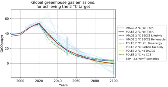
Figure ES.1. Global greenhouse gas emissions under the 2 °C and 1.5 °C Full technology and alternative scenarios of IMAGE and POLES, compared to the full set of cost-optimal SSP 2.6 W/m2 _{and 1.9 W/m}2 _{scenarios (i.e. pathways leading to a radiative forcing level of 2.6 W/m}2

and 1.9 W/m2 _{by 2100) (Rogelj et al., 2018). Vertical bars indicate the SSP scenario ranges}

for 2050 and 2100.

It is technically possible to rely less on negative emission technologies and bio-energy than is the case under the Full technology scenarios and still meet stringent climate goals. This report explores some alternative scenarios for achieving 2 °C and 1.5

°C targets that rely less on BECCS and bio-energy. These scenarios show that it is possible to decrease the dependence on bio-energy and BECCS, using alternative reduction options and timely efforts. Less reliance on BECCS can be achieved, for instance, through further penetration of renewable energy, rapid energy efficiency improvements, lifestyle changes, more reforestation and more rapid reduction in non-CO2 gases. This report presents such

scenarios, as explored using the IMAGE model. For instance, with respect to lifestyle

changes, a scenario is presented that looks at a shift towards low-meat diets, which leads to fewer land-use-related CO2 emissions and non-CO2 greenhouse gas emissions. Several of

the scenarios that use less BECCS assume that sequestration is achieved via other CDR options, such as reforestation and the application of CCS.

Nevertheless, under all scenarios presented here, in order to achieve the 1.5 °C target, net emissions still need to become negative during the second half of this century. Emission levels under most alternative scenarios are lower before mid century and

higher at the end of the century, compared to their respective Full technology scenarios. The entire 2050 emission range, for the Full technology and alternative scenarios, results in a

reduction of between 51% to 63% (for the 2 °C target) and between 70% and 82% (for the 1.5 °C target), below 1990 levels (Figure ES.1).

For the EU, emission reductions consistent with achieving the 2 °C and 1.5 °C targets are about 80% and 90%, respectively, below 1990 levels, by 2050, under the Full

technology scenarios that assume reductions are implemented efficiently and on a

global scale, beyond 2020. For the EU, the Full technology and alternative 2 °C scenarios

show a reduction range of between 76% and 84% by 2050, below 1990 levels. The Full technology and alternative 1.5 °C scenarios show reductions of about 91% by 2050. For target setting, equity considerations can also be included. Scenarios based on equity principles other than cost efficiency lead to higher reductions, in high-income regions.

1 Introduction

Under the Paris Agreement (December 2015), nearly all countries in the world agreed to limit global temperature increase to well below 2 °C above pre-industrial levels, and to pursue efforts to limit this increase even further to 1.5 °C (UNFCCC, 2015). Mitigation scenarios in the literature that achieve the climate targets of 1.5 °C and 2 °C show deep reductions in greenhouse gas emissions and rely on net Carbon Dioxide Removal (CDR) from the

atmosphere, mostly accomplished through large-scale use of bio-energy with carbon capture and storage (BECCS) and afforestation (Luderer et al., 2018; Riahi et al., 2017; Rogelj et al., 2017; Rogelj et al., 2018; van Soest et al., 2017; van Vuuren et al., 2017; Vrontisi et al., 2018). However, important challenges have been identified for large-scale application of negative emission technologies. This includes possible trade-offs between production of bio-energy, food and protection of biodiversity, all depending on limited land and water

resources (Foley et al., 2005; Hasegawa et al., 2018). Given these limitations, CDR technologies cannot be applied without restriction, as there are limits to afforestation, bio-energy generation and carbon storage (Smith et al., 2016).

The question arises whether alternative deep mitigation pathways to limit warming to 1.5 °C and 2 °C above pre-industrial temperatures relying on less use of negative emissions from BECCS and afforestation exist. Van Vuuren et al. (2018) used the integrated assessment model IMAGE (Stehfest et al., 2014) to investigate BECCS specifically, and explored the impact of alternative pathways for meeting 1.5 °C that include lifestyle change, additional reduction in non-CO2 greenhouse gases and more rapid electrification of energy demand

based on renewable energy. Van Vuuren et al. concluded that these options significantly reduce the need for CDR, but not fully eliminate it. The role of bio-energy in these 1.5 °C pathways was investigated to a lesser extent, and 2 °C scenarios were beyond the scope of their work. Furthermore, the results were obtained through scenario calculations using one integrated assessment model.

This study builds upon earlier research, but specifically focuses on strategies to meet the Paris climate objective as well as scenarios that could limit the use of bio-energy and BECCS. Both the IMAGE and POLES suites aim for the same climate targets and both include Full-technology scenarios and scenarios that limit the deployment of BECCS. They do so however through different, but complementary, protocols. The IMAGE pathways present a world in which the additional use of renewables and lifestyle changes lower the need for BECCS deployment. The pathways calculated with the POLES model limit the availability of bio-energy overall which eventually leads to less use of BECCS, and consequently, more

electrification and penetration of non-bio-energy renewables. We have structured the report to address the following two main research questions:

1) How do scenarios consistent with the Paris climate objective look like in terms of global energy use and production, land use, and emissions under full-technology assumptions, and what is the role of mitigation options BECCS and bio-energy in these scenarios?

2) Can we also develop emission pathways for meeting 2 °C and 1.5 °C that rely less on BECCS and bio-energy?

The scenarios were run by two different integrated assessment models, i.e. IMAGE and POLES. In addition to the overall results, we present the outcomes for the land-use system and some of the implications at the regional European scale.

This report is structured as follows: Chapter 2 describes the methodology and the scenarios. Chapter 3 analyses the Full technology scenarios that that limit warming to well below 2 °C or to 1.5 °C using the IMAGE and POLES models, and tries to address the first main research question. Chapter 4 explores alternative scenarios for meeting 2 °C and 1.5 °C, that rely less on BECCS and bio-energy, and thereby tries to address the second main research question of this report. Chapter 6 discusses the implications for the land-use sector. Finally, chapter 6 briefly discusses the changes in the energy use and production, and greenhouse gas emissions for the EU.

Box 1. Emission scenarios

The IPCC defines such scenarios as a plausible representation of the future development of emissions of substances that are potentially radiatively active (e.g., greenhouse gases, aerosols) based on a coherent and internally consistent set of assumptions about driving forces (e.g. demographic and socio-economic development, technological change) and their key relationships’. In other words, such scenarios are used to explore different possible trajectories for future emissions based on a set of key assumptions. Many scenarios, in fact, explore technically feasible and low-cost pathways towards achieving particular policy goals (e.g. the Paris climate objective). While scenarios normally depict pathways that are technically and economically feasible, the model outcomes say little about political or social feasibility. It should also be noted that scenarios are not meant to form a direct input for target setting. Targets are usually based on a much broader set of considerations than only technical and economic criteria.

2 Modelling set-up

Introduction

For the IMAGE analysis, the IMAGE 3.0 model was used. The IMAGE scenarios presented are either default (i.e. full technology, low-cost) pathways for reaching the Paris climate

objective or the scenarios based on the recent work done on alternative 1.5 °C scenarios (lifestyle changes, more renewables & electrification) (van Vuuren et al., 2018), with the latest model updates on the electricity model. JRC used the POLES-JRC model starting from the GECO2017 model version (Kitous et al., 2017) with in addition recent model upgrades that will be used in the up-coming GECO2018 report: end uses in buildings, power system, oil and natural gas production module. The POLES scenarios presented here were finalised in July 2018. Both models are briefly described below.

Model description

2.2.1 IMAGE model

IMAGE 3.0 is a comprehensive ecological-environmental model framework that simulates the environmental consequences of human activities worldwide (Stehfest et al., 2014; van Vuuren et al., 2017; van Vuuren et al., 2018). It represents interactions between society, the biosphere and the climate system to assess sustainability issues such as climate change, biodiversity and human well-being. The model is a simulation model, i.e. changes in model parameters are calculated on the basis of the information from the previous time step. The model includes a detailed description of the energy and land-use system and simulates most of the socio-economic parameters for 26 regions and most of the environmental parameters on the basis of a geographical grid of 30 x 30 minutes or 5 x 5 minutes (depending on the variable). Important inputs to the model are descriptions of the future development of so-called direct and indirect drivers of global environmental change. Exogenous assumptions on population, economic development, lifestyle, policies and technology change form a key input into the detailed energy system model TIMER and the food and agriculture system, including the agro-economic model MAGNET.

The IMage Energy Regional model, also referred to as TIMER, has been developed to explore scenarios for the energy system in the broader context of the IMAGE global environmental assessment framework (van Vuuren, 2007; van Vuuren et al., 2017). TIMER describes 12 primary energy carriers in 26 world regions and is used to analyse long-term trends in energy demand and supply in the context of the sustainable development challenges. The model simulates long-term trends in energy use, issues related to depletion, energy-related greenhouse gas and other air polluting emissions, together with land-use demand for energy crops. The focus is on dynamic relationships in the energy system, such as inertia and learning-by-doing in capital stocks, depletion of the resource base and trade between regions.

In IMAGE, the main interaction with the earth system is by changes in energy, food and biofuel production that induce land-use changes and emissions of carbon dioxide and other greenhouse gases. The calculated emissions of greenhouse gases and air pollutants are used

in IMAGE to derive changes in concentrations of greenhouse gases, ozone precursors and species involved in aerosol formation on a global scale. Climatic change is calculated as global mean temperature change using a slightly adapted version of the MAGICC 6.0 climate model (Meinshausen et al., 2011a).

2.2.2 POLES model

The POLES-JRC (Prospective Outlook on Long-term Energy Systems) model is a global partial equilibrium simulation model of the energy sector, with complete modelling from upstream production through to final user demand (Keramidas et al., 2017; Vandyck et al., 2016). The POLES-JRC model follows a year-by-year recursive modelling, with endogenous international energy prices and lagged adjustments of supply and demand by world region, combining price-induced mechanisms with a detailed technological description and technological change in several sectors, in particular electricity generation. The model covers 39 regions around the world, including the EU. The model covers 15 fuel supply branches, 30 technologies in power production, 6 in transformation, 15 final demand sectors and corresponding

greenhouse gas emissions. Population and GDP is an exogenous input into the model, while endogenous resource prices, endogenous global technological progress in electricity

generation technologies and price-induced lagged adjustments of energy supply and demand are important features of the model. The power sector includes an explicit representation of hourly load curve for representative days and investment decisions for capacity planning, taking into account constraints of technical availability (not yet mature technology, base/peak load) and technology-relevant potential (hydropower, wind, solar, bio-energy, CCS geological storage). Electricity storage (including flexible demand) develops within the space defined by the load curve and the intermittent supply of renewables in each hourly step. Penetration of synthetic fuels is defined by their cost-competitiveness, with a

representation of production costs and infrastructure costs (where relevant, e.g. hydrogen). The mitigation policies discussed in the report are implemented by introducing carbon prices up to the level where emission reduction targets are met. Carbon prices affect the average energy prices, inducing energy efficiency responses on the demand side, and the relative prices of different fuels and technologies, leading to adjustments on both the demand side (e.g. fuel switch) and the supply side (e.g. investments in renewables).

The POLES-JRC model was specifically designed for the energy sector but also includes other greenhouse gas emitting activities. Non-CO2 emissions in energy, industry and agriculture

and CO2 emissions from the land-use sector (land use, land-use change, and forestry

(LULUCF) and agriculture) follow a cost curves approach. The land-use sector interact with the energy sector via the supply and demand of different forms of bio-energy; emission levels are determined by climate policies (marginal abatement cost curve, from GLOBIOM (Havlík et al., 2014) and bio-energy supply levels (marginal cost curve, also from GLOBIOM). GLOBIOM covers major greenhouse gas emissions from agricultural production, forestry, and other land use including CO2 emissions from above- and below-ground biomass changes,

N2O from the application of synthetic fertiliser and manure to soils, N2O from manure

dropped on pastures, CH4 from rice cultivation, N2O and CH4 from manure management,

and CH4 from enteric fermentation. More stringent climate policies result in increased

competitiveness of energy due to its low carbon content, and in a higher demand for bio-energy. This, in turn, leads to higher bio-energy prices, increased bio-energy supply to the energy sector in generally, and, in the absence of climate policies, to more land-use emissions. The bio-energy price and land-use emissions result from these interactions. A large part of the greenhouse gas mitigation potential in LULUCF and agriculture is accessible at low cost, and with relatively minor feedback due to an increased demand for bio-energy. Historical agriculture emissions are harmonised with the emissions from national statistics (FAO); historical LULUCF emissions are directly derived from GLOBIOM (which itself follows national inventory and FAO data). Forest management emissions consider that harvested wood results in emissions and removals upon production; in the rest of the model,

combustion of solid bio-energy is considered carbon-neutral (and BECCS is considered carbon-negative to the amount of an average bio-energy carbon content) while liquid biofuels consider conversion efficiencies and transformation energy use in their carbon content.

Finally, the mitigation options for the agriculture sector (as estimated by GLOBIOM1_{), in}

more detail:

 Technical non-CO2 mitigation options are included in the model based on the

mitigation option database from EPA (Beach et al., 2015) and include: improved fertiliser management, nitrogen inhibitors, improved feed, conversion efficiency, feed supplements (i.e. propionate precursors, anti-methanogen), changes in herd management (i.e. intensive grazing), improved manure management ( i.e. anaerobic digesters).

 Structural mitigation options (Havlík et al., 2014) are explicitly represented in the model via four different crop management systems ranging from subsistence farming to high input systems with irrigation technology. For the livestock sector, an extensive set of production systems from extensive to intensive management practises is available based on Herrero et al. (2013). This allows the model to switch between management practises in response to e.g. a carbon price and hence decrease emissions through greenhouse gas efficient intensification. The model may also reallocate production to more productive areas within a region or even across regions through international trade.

 The impact of changes in commodity prices on the demand side is explicitly considered and consumers’ react to increasing prices by decreasing consumption depending on the region-specific price elasticities (Muhammad et al., 2011).

The mitigation options for the LULUCF sector (as estimated by GLOBIOM2_):

 Reduction in deforestation activities.

 Increase in afforestation activities and afforested areas.

 Changes in rotation length of existing managed forests in different locations.  Changes in the ratio of thinning versus final felling.

 Changes in harvest intensity (amount of biomass extracted in thinning and final felling activity).

1 _{For further information about the mitigation options for the agriculture sector as considered within GLOBIOM,} we refer to Frank et al. (2018).

2 _{For further information about the about the mitigation options for the LULUCF sector as considered within} GLOBIOM we refer to Havlík et al. (2014).

General scenario formulation

The IMAGE and POLES models can assess the implications of various mitigation strategies, in terms of changes in energy system, land use, emissions and associated costs. The IMAGE and POLES models can be used to design baseline scenarios (no climate policies), current policies scenarios and mitigation scenarios that can meet the climate targets of 1.5 °C and 2 °C, at certain probabilities, i.e.:

1. The 2 °C scenarios: keeping global warming below 2 °C in the 21st century, with a probability of at least 66%

2. The 1.5 °C scenarios: keeping global warming below 1.5 °C in 2100, with a probability of at least 50%

The baseline, current policies and mitigation scenarios are represented in the models IMAGE and POLES in different ways, as briefly described below. For the 1.5 °C and 2°C scenarios, we assume different assumptions around the use of BECCS, CCS and bio-energy, as will be described in Section 3.2.

2.3.1 IMAGE model

The IMAGE model is used for exploring mitigation scenarios for achieving the 1.5 °C and 2 °C climate targets, leading to a radiative forcing of 1.9 and 2.6 W/m2 _{by 2100.}

The IMAGE scenarios analysed here are all based on the IMAGE implementation of the SSP2 baseline scenario (van Vuuren et al., 2017), which is the IMAGE baseline (no policy) scenario in the analysis. The SSP2 scenario describes a middle-of-the-road scenario in terms of economic and population growth and other long-term trends, such as in technology development. The main drivers of this scenario for the energy and industrial sectors are population, gross domestic product (GDP), lifestyle and technology change.

The IMAGE current policies scenario was derived from the original SSP2 baseline by

introducing explicit policy measures, and is reported in detail in Roelfsema et al. (2018), van Soest et al. (2017) and Kuramochi et al. (2017). This scenario assumes that current policies are implemented up to 2030. For the 2030–2100 period, the scenario assumes no new policies. Policies may have a long-term effect through the induced technology learning effects (e.g. by additionally installed renewable energy technologies compared to the SSP2 baseline). Mitigation efforts in the land-use sector assume an implementation of a low-carbon tax in the sector, to enhance REDD and to increase reforestation of half of the degraded forest, as described in more detail in Doelman et al. (2018).

In the standard set-up of the model for the mitigation scenarios, the mitigation scenarios are implemented by a universal global carbon tax in all regions and sectors, which is

implemented from 2020 onwards, in order to reach the radiative forcing targets following a cost-optimal pathway. Before 2020, all mitigation scenarios assume the full implementation of the countries’ reduction proposals (conditional pledges) for 2020, as part of the Cancun Agreements (based on den Elzen et al. (2016) and the IMAGE implementation, as described in van Soest et al. (2017).

In terms of mitigation in the energy system TIMER covers a wide range of mitigation options, including a major shift from a system mostly based on fossil fuels to an increase in the use of nuclear power, renewable energy (different solar and wind technologies, hydropower), bio-energy (first and second generation), nuclear power and CCS technology, with a

In terms of land-based mitigation options, IMAGE accounts for three general types of options: bio-energy production, REDD (avoided deforestation) and reforestation of degraded forests. Bio-energy demand is determined by TIMER based on bio-energy yield, the carbon price, dynamics in the energy system, and land availability, following a food-first principle (Hoogwijk et al., 2009).

The demand for bio-energy in climate change mitigation scenarios is thereby directly linked to the carbon price required to reach the scenario-specific mitigation target (van Vuuren et al., 2017). More specifically, bio-energy is one of the energy carriers that competes to supply the demand for energy. In combination with carbon capture and storage (BECCS), bio-energy enables the production of negative emissions, by storing carbon that is captured from the atmosphere in the form of biomass. The price and amount of bio-energy in the model, is based on information from the IMAGE land system. The deployment of BECCS occurs in the electricity, hydrogen and industry sectors that adopt the use of BECCS according to its competitive position

REDD is implemented by protecting areas with high carbon stocks according to Ruesch and Gibbs (2008), thereby limiting the total amount of land available for producing food, feed and fibre. Three increasingly strict protection levels are defined at 200, 150 and 100 tC/ha. Reforestation on degraded forest areas restores areas that have been degraded for reasons other than agriculture (e.g. unsustainable forest management, mining, illegal logging). Two levels of reforestation are defined as mitigation options: either half or all of the degraded forest areas are reforested. The level of REDD and reforestation are scenario-specific (linked to the climate target) and thereby only indirectly linked to the carbon price. However, the mitigation level has been roughly calibrated to abatement curves on avoided deforestation as calculated by IIASA (Kindermann et al., 2008). For further details concerning the migration options we refer to Doelman et al. (2018).

Table 1: Levels of REDD and reforestation assumed to be implemented for mitigation targets. The data below is specific for the SSP2 scenario.

Climate target (W/m

_{) REDD*}

_{Reforestation**}

1.9

High REDD

Full reforestation

2.6

Medium REDD Full reforestation

3.4

Low REDD

Half reforestation

4.5

No REDD

No reforestation

6.0

No REDD

No reforestation

* REDD is defined using a carbon density threshold: high REDD: 100 tC/ha, medium REDD: 150 tC/ha, low REDD: 200 tC/ha.

** Full reforestation assumes that all degraded forests are restored, half reforestation assumes that half of degraded forests are restored.

In non-CO2 greenhouse gases, IMAGE utilises the cost curves approach to account for the

future maximum attainable reduction potential and associated costs for these sources of emissions (see Lucas et al., 2007). The cost supply curves accounts for option-specific technical mitigation potentials and costs for CH4 and N2O emissions from agriculture

sources. Technological options as accounted for in the cost supply curves includes options to reduce CH4 emissions from rice production, enteric fermentation and animal waste, and

2.3.2 POLES model

The POLES scenarios presented here were finalised in July 2018. The POLES model explored emission pathways for achieving 1.5 °C and 2 °C targets. The scenarios were run through MAGICC 6.0 climate model3 _{(Meinshausen et al., 2011a) and a carbon budget that was}

derived from multiple scenario runs with the targets of keeping warming below the 2 °C and 1.5 °C with a 66% probability, as defined by online MAGICC probabilistic runs4_{. The}

cumulative anthropogenic CO2 emissions for the 2010–2100 period are around 1150 GtCO2

for the 2 °C target, which is higher than the IMAGE projections (about 1000 GtCO2 for 2 °C),

and around 500 GtCO2 for the 1.5 °C target, which is similar to the IMAGE projections

(Appendix A).

The POLES current policies scenario is based on the GECO2017 Reference scenario (Kitous et al., 2017). It includes adopted energy and climate policies worldwide, for 2020, and the extension of the EU ETS to 2050 (with a constantly decreasing cap at -1.74%/yr); after 2020, CO2 and other greenhouse gas emissions are driven by income growth, energy prices

and expected technological development with no supplementary incentivising for low-carbon technologies (Kitous et al., 2017). A full list of the policies considered for the GECO2017 Reference scenario, and their implementation are provided in Annex 5 of the GECO2017 report (Kitous et al., 2017).

The POLES low-carbon scenarios analysed here are all based on the POLES current policies scenario. In the standard set-up of the model, the mitigation scenarios are implemented by a carbon tax, sectoral measures and policies, in all regions and sectors. The main assumptions are described below.

Carbon price:

- Increases over time at a decreasing annual rate

- Carbon price by country is differentiated according to per capita income until 2050, same price afterwards

- AFOLU sector (derived from GLOBIOM lookup tables): carbon price limited (where necessary) to maximum carbon price point provided by GLOBIOM5

- All other sectors are subject to the same carbon price

3 _{According to MAGICC, see: http://live.magicc.org/ The results presented here used the online version of} MAGICC as of October 2018 (nominally this is MAGICC 6.0).

4 _{Temperature responses to CO2 concentrations, CO2 budgets, the accounting of land use CO2 emissions and} probabilities of reaching a temperature target from MAGICC, in particular those relating to 1.5 °C, should be reassessed in the future with input from new literature, e.g. the IPCC 1.5 °C Special Report.

5 _{In order to consider the mitigation potential within the AFOLU sector, POLES need information about the} economic potential for AFOLU mitigation. This, together with information about the economic potential for biomass supply and the related emissions, is provided by GLOBIOM in the form of lookup tables. These lookup tables jointly provide two critical pieces of information: i) the economic potential for biomass supply in the form of a supply function where the supplied quantity is a function of biomass price, ii) the economic mitigation potential is described in the form of marginal abatement cost supply curves where the emission reduction is a function of the carbon price. For a specific carbon and biomass price development, the lookup tables thereby provide the full information about the development of the AFOLU sector. In the standard set up, the mitigation potential within the land-use sector is quantified according to a total of 12 carbon price steps ranging from 0 USD/tCO2eq to a maximum of 2000 USD/tCO2eq.

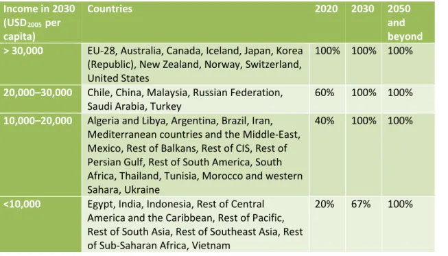
Table 2: Carbon price differentiation in POLES scenarios

Income in 2030

(USD2005 per

capita)

Countries

2020 2030 2050

and

beyond

> 30,000

EU-28, Australia, Canada, Iceland, Japan, Korea

(Republic), New Zealand, Norway, Switzerland,

United States

100% 100% 100%

20,000–30,000

Chile, China, Malaysia, Russian Federation,

Saudi Arabia, Turkey

60% 100% 100%

10,000–20,000

Algeria and Libya, Argentina, Brazil, Iran,

Mediterranean countries and the Middle-East,

Mexico, Rest of Balkans, Rest of CIS, Rest of

Persian Gulf, Rest of South America, South

Africa, Thailand, Tunisia, Morocco and western

Sahara, Ukraine

40% 100% 100%

<10,000

Egypt, India, Indonesia, Rest of Central

America and the Caribbean, Rest of Pacific,

Rest of South Asia, Rest of Southeast Asia, Rest

of Sub-Saharan Africa, Vietnam

20% 67% 100%

Sectoral measures:

- Buildings:

 increased rate of renewal of the stock and of renovation of existing surfaces  new and renovated surfaces move closer to best-available practices in terms of

insulation (country-dependent on the basis of heating and cooling degree days and energy prices)

- Transport:

 Scenarios assume gradual development of refuelling infrastructure and consumer acceptance over time for electric vehicles

 Private passenger vehicles: emissions per kilometre travelled in newly sold vehicles per country follow the decreases in emissions per kilometre, due to the fuel or emission standards for vehicles of EU average new sales, as defined by EU regulation on CO2 emissions from passenger vehicles 2007–2021 and 2021–2030 (10-year delay

for non-OECD)

 Road freight: the decreases in emissions per kilometre across the EU car fleet, over 2007–2021 and 2021–2030, are used as a basis for the decreases in emissions from freight transport, with a 10-year delay (20-year delay for non-OECD)

- Industry:

 Energy efficiency value (differentiated across countries on income per capita)

Policies:

 Copenhagen pledges (2020) and several energy-related policy targets announced in the NDCs (renewables deployment) are reached or exceeded (2025–2035)

 Carbon prices are at least of a level necessary for reaching the NDC emission level (2025–2035)

 Maritime freight: the IMO objective for 2050 (-50% vs 2008) is achieved

 HFCs: the reduction targets as prescribed by the Kigali Amendment to the Montreal Protocol are reached

Mitigation scenarios for meeting 1.5 °C and 2 °C

targets

Different mitigation scenarios were constructed, along a temperature axis (2 °C or 1.5 °C maximum increase) and a technology axis (mix of technological constraints).

The low-carbon scenarios were calculated for the two climate targets (2 °C and 1.5 °C): 1. The below 2 °C scenarios: keeping global warming below 2 °C in the 21st century

with a probability of at least 66% and varying availability of mitigation options, i.e. the use of BECCS, CCS and bio-energy, and alternatively, lifestyle changes.

2. The 1.5 °C scenarios: keeping global warming to 1.5 °C in 2100 with a probability of at least 50% and varying availability of mitigation options. These scenarios show a global mean average temperature increase with a limited overshoot of the 1.5 °C target by about 0.2–0.3°C, before returning to 1.5 °C by 2100.

A general description of the technological constraints is listed in Table 3.

Both models have Full technology 2 °C and 1.5 °C scenarios. The IMAGE Full technology 2 °C and 1.5 °C scenarios are described in detail in van Vuuren et al. (2018) (see IMAGE default 1.9 and 2.6 Wm2 _{scenarios). In the POLES model, ambitious levels of bio-energy are}

assumed according to GLOBIOM, of <300EJ/yr by 2100. All POLES scenarios here could be considered as having limited CCS, as the model assumes a delay of the emergence of CCS technologies and limits the annual growth potential for CCS. The POLES scenarios all assume DACCS6 _{(with the exception of the No DACCS and No CCS scenarios), first available from}

2040; by 2100 can be limited by regional geological storage potential (no physical trade of CO2).

The IMAGE Limited BECCS – Renewable electricity scenario and the POLES Limited

Bio-energy, Limited Bio-energy – No CCS scenarios are somewhat comparable, in terms of

BECCS implementation. Under the POLES scenario, the limited bio-energy availability results in limited BECCS. Ambitious levels of bio-energy, as under the POLES Full technology scenarios, result in more BECCS, given the emission constraints in these scenarios.

The IMAGE Limited BECCS – Lifestyle change scenario assumes a lifestyle change that leads to a less meat-intensive diet, as well as a full package of lifestyle changes. The scenario includes dietary change, food waste reduction and changes in transportation and residential energy use. For dietary change, we assume a quick transition to a healthier diet (the so-called Wilett diet) between 2020 and 2050, with low levels of meat consumption (van Sluisveld et al., 2016). Earlier implementations of this scenario have been described in detail (Bijl et al., 2017; van Vuuren et al., 2018).These sets of assumptions are for IMAGE only

included in the Lifestyle scenario. In POLES, all scenarios include a food security constraint to avoid strong decreases in calorie intake (especially in developing countries) under high carbon prices on AFOLU emissions, which increase agricultural prices for greenhouse gas intensive products such as ruminant meat, milk, or rice. This constraint basically ensures that by 2030 the population at risk of hunger cannot be higher than 1% in developing countries. This constraint is in line with SDG2 Zero Hunger of around 10% in 2016 according to FAOSTAT. The food security constraint forces a certain level of calorie intake for vegetal and animal calories corresponding to an undernourishment of maximum 1% by 2030. If developing countries exceed this calorie intake threshold over time, they may reduce their consumption levels because of the carbon price response to that threshold, or they may not. Developed regions are able to decrease their calorie intake to 2010 consumption levels.

Table 3: Description of the mitigation scenarios included in this analysis, for 2 °C and 1.5 °C, in the IMAGE and POLES model

Scenario name

Scenario description IMAGE SSP2

baseline

IMAGE implementation of the SSP2 scenario.

IMAGE current policies

Implementation of current policies until 2030 and constant reduction effort (compared to IMAGE SSP2 baseline) between 2030 and 2100.

POLES current policies

Implementation of current policies until 2020; no additional policies beyond 2020. Scenario name Scenario description IMAGE 2 °C Full technology

Full technology implementation with a universal global carbon tax in all regions and sectors from 2020 onward. Selection of technologies based on relative costs.

POLES 2 °C Full

technology

Full technology implementation with a carbon tax in all regions and sectors from 2018 onward (differentiated by region, uniform from 2050).

Selection of technologies based on relative costs. IMAGE 2 °C

Limited BECCS – Lifestyle change

Limited deployment of BECCS through implementation of lifestyle changes. Consumers change their habits towards a lifestyle that leads to lower greenhouse gas emissions. This includes a less meat-intensive diet (conform health recommendations), less CO2-intensive transport modes

(following the current modal split in Japan), less intensive use of heating and cooling (change of 1 °C in heating and cooling reference levels) and a reduction in the use of certain domestic appliances. It assumes further optimistic afforestation levels from the SSP1 scenario.

IMAGE 2 °C Limited BECCS – Renewable electricity

Limited deployment of BECCS through higher electrification rates in all end-use sectors, in combination with optimistic assumptions on the integration of variable renewables and on costs of transmission, distribution and storage.

POLES 2 °C Limited Bio-energy

Limited availability of bio-energy (<180 EJ/yr, all years) achieved by additional demand-side measures targeted at bio-energy use.

POLES 2 °C Carbon tax only

Similar to the POLES 2 °C Limited Bio-energy scenario. However, the only mitigation measure applied is that of carbon pricing, uniformly

specific measures on a sectoral level (e.g. vehicle fuel standards), hence a higher carbon tax level.

POLES 2 °C Limited Bio-energy – No DACCS

Similar to the POLES 2 °C Limited Bio-energy scenario, without deployment of DACCS

POLES 2 °C Limited Bio-energy – No CCS

Similar to the POLES 2 °C Limited Bio-energy scenario, without deployment of CCS. Scenario name Scenario description IMAGE 1.5 °C Full technology

Full technology implementation with a universal global carbon tax in all regions and sectors, from 2020 onward. Selection of technologies based on least-cost options.

POLES 1.5 °C Full

technology

Full technology implementation with a differentiated carbon tax in all regions and sectors, from 2018 onward (differentiated by region, universal from 2050). Selection of technologies based on least-cost options.

IMAGE 1.5 °C Limited BECCS – Lifestyle change

Limited deployment of BECCS through implementation of lifestyle changes.

IMAGE 1.5 °C Limited BECCS – Renewable electricity

Limited deployment of BECCS through higher electrification rates and implementation of renewables.

POLES 1.5 °C Limited Bio-energy

Limited availability of bio-energy for energy (<180 EJ/yr, all years) achieved by additional demand-side measures targeted at bio-energy use.

2.4.1 Model implementation of scenarios

As a full technology configuration, the implicit "subsidy" of BECCS, in the POLES model resulting from the negative carbon emissions, was capped for example to ensure that despite this "carbon subsidy" the electricity with BECCS is not produced at a negative or zero cost7_.

In addition, to limit the diffusion of BECCS, the JRC has limited the overall availability of ‘bio-energy-for-energy’ in all demand sectors. As a result, more electrification and penetration of non-bio-energy renewables is expected.

Conversely, the PBL IMAGE model used the opposite set-up by introducing alternative activity development and energy option availability, i.e. lifestyle changes and more electrification and renewables, leading to lower BECCs. For example, for the lifestyle scenario, we first apply the lifestyle change assumptions in the IMAGE model, leading to a lower emission trend compared to the SSP2 emission projections. Applying the same carbon tax as under the Full technology scenarios of 1.9 and 2.6 W/m2 _{will lead to radiative forcing}

levels by 2100 of below the target levels of 1.9 and 2.6 Wm2_{. In order to meet these}

7 _{BECCS as a sequestration technology would generate revenue from electricity sales and “carbon revenue” as a} consequence of it being a net-negative emissions technology; this would potentially crowd out other generation technologies. This effect is limited in the model by using BECCS only in certain parts of the load (after wind and solar contribution and not during peak load hours) and by assuming BECCS is deployed only up to the point where it becomes competitive with the cheapest centralized electricity generation technology (but not beyond this point).

radiative forcing targets levels, a premium factor on the use of BECCS is introduced. The final level is calculated through an iterative process of multiple runs, in which each time the factor is continuously increased until the required forcing levels are reached.

While the POLES model showed that all selected 2 °C scenarios are feasible, two scenarios run with the IMAGE model were “infeasible”. These were a 2 °C No CCS and 2 °C No

BECCS scenario that do not permit the deployment of the respective technologies. An

“infeasible” scenario means that a specific model in our set could not find a solution given the combination of limited action until 2020, and meeting the radiative forcing targets for the IMAGE, and the carbon budget targets for the POLES scenario. Infeasibilities may occur due to different reasons, such as lack of mitigation options to stay within the carbon budget or radiative forcing constraints or binding constraints for the diffusion of technologies (Riahi et al., 2015).

In the context of the 1.5 °C target, significantly fewer scenarios were found to be feasible. The POLES model only found feasible scenario outcomes under the Full Technology and Limited Bio-energy scenarios, and the IMAGE model found feasible outcomes only under the Full Technology and two Limited BECCS scenarios.

3 Current policies and

Full technology

mitigation scenarios

Current policies scenarios

Findings

 The IMAGE and POLES global models have similar greenhouse gas emission

projections under Current policies scenarios until 2030. After 2030, however, their projections diverge due to different assumptions about the post-2030 period.

 Bio-energy use, under the Current policies scenarios, increases throughout the

century in both models, with a 62% increase by 2100 (compared to 2010) under the IMAGE Full technology scenario and a 71% increase under the POLES scenario.

Results

This section compares the IMAGE Current policies scenario, as described in detail in Roelfsema et al. (2018), van Soest et al. (2017) and Kuramochi et al. (2017), with the POLES Current policies scenario. This IMAGE scenario assumes that current policies are implemented up to 2030, and that after 2030, the induced technology learning effects will lead to around 5% reduction in greenhouse gas emissions (excluding those from land use), compared to the IMAGE SSP2 baseline scenario. Mitigation efforts in the land-use sector also lead to enhanced REDD and increased reforestation of half the degraded forest, as described in more detail in Chapter 5 and in Doelman et al. (2018).

POLES assumes a different pathway for their current policies scenario in which current policies are implemented up to 2020 (except for the EU ETS, which is extended to 2050) and market prices and technological development drives emissions until the end of the century, resulting in roughly stable emissions from the 2050s onwards.

Figure 1. Global greenhouse gas emissions (panel a and b) and primary energy demand by energy carrier (panel c and d) for the IMAGE and POLES current policies (Ref.) scenarios

The top left plot of Figure 1a shows the development of total greenhouse gas emissions over time for the IMAGE and POLES current policies scenarios. It shows that both models have similar greenhouse gas emission projections of current policies scenarios until 2030, but after 2030, their projections diverge due to different assumptions about the post-2030 period. The relative reduction under the IMAGE current policies scenario, compared to the SSP2 baseline, is about 5%. The greenhouse gas emissions under the POLES current policy scenario

stabilises after 2030.

Figure 1b shows the individual greenhouse gas emissions in 1990, 2010 and 2030 for both models. Breaking down the greenhouse gas emissions into separate gases, and

differentiating between CO2 emissions from the energy and land-use sectors, shows that

main differences can be found in land-use-related CO2 emissions (i.e. CO2 emissions from

land-use changes and removals). These emissions are lower under the POLES reference scenario, as a result of the use of the historical land-use emission estimates from national inventories. The latter are lower than the historical land-use emissions as simulated in integrated assessment models (Grassi et al., 2017) (see Section 5.1). Figure 1c and 1d (bottom two plots of the figure) shows the primary demand for current policies for both models. The historical primary energy demand is about the same for both models, which is expected as both models are calibrated on energy demand data from IEA. The breakdown into energy carriers reveals that the models assume that different technological pathways to evolve over the course of the century. POLES achieves the constant Kyoto emissions by switching from a fossil-dominated energy mix to one in which renewables play a larger role.

Even in the absence of targeted climate mitigation policies renewables become

cost-competitive against fossil fuel use in many regions of the world for the POLES scenario. This is not the case for the IMAGE scenario. In the current policy scenario, coal is still a dominant energy by the end of the century. Both models however show that the use of bio-energy increases (with and without CCS), with an increase of 41% and 62% in 2050 and 2100 compared to 2010 for IMAGE and 54% and 71% in 2050 and 2100 compared to 2010 for POLES. The use of bio-energy combined with CCS however is negligible in both scenarios. BECCS does not become cost-competitive and plays no role in a world in which no additional mitigation efforts are required.

The 2 °C Full technology scenarios

Findings

 Model-based scenarios show that Full technology scenarios existin which all technologies are assumed to be available that limit global warming to below 2 °C in the 21st century, with at least 66% probability.

 The Full technology 2 °C scenarios of IMAGE and POLES reach emissions of 2.8

and -0.7 GtCO2eq/yr by 2100. The POLES 2 °C scenario reaches greenhouse gas

neutrality (net zero greenhouse gas emissions) after 2090. Greenhouse gas emissions are reduced by a respective 56% and 51% by 2050, from 1990 levels, under the 2 °C Full technology IMAGE and POLES scenarios.

 Global greenhouse gas emissions under the IMAGE and POLES Full technology

2 °C scenarios are in the lower emission range for 2050, and in the upper range for 2100 of all full technology 2.6 W/m2 _{scenarios from all global models based}

on the SSP multi-model comparison study (Rogelj et al., 2018).

 Full technology scenarios rely on rapid and deep emission reductions through a

mix of energy efficiency, rapid introduction of energy options without CO2

emissions (e.g. renewable energy and CCS), negative emission options (e.g. bio-energy with CCS (BECCS) and afforestation) and reduction in non-CO2

greenhouse gas emissions. The IMAGE 2 °C scenario has a higher contribution of energy efficiency improvements and CCS, whereas the POLES 2 °C scenario relies more on rapid penetration of renewable energy technologies.

 The increase in bio-energy use is substantial in both models, but higher in the

POLES scenario due to the greater availability of biomass for energy.

 In the IMAGE scenario, CCS is being deployed early and the share between

fossil fuel and bio-energy with CCS is roughly evenly distributed. In the POLES scenario, CCS is deployed later and is dominated by BECCS.

Results

For the analysis of the 2 °C scenarios, the two models assume different climate constraints. The IMAGE model is used to explore 2 °C emission pathways assuming that radiative forcing reaches 2.6 W/m2 _{by 2100, whereas the POLES model explores 2 °C pathways by finding the}

cumulative anthropogenic CO2 emissions for the 2010–2100 period compatible with that

maximum temperature increase (according to MAGICC). As a result, the cumulative CO2

emissions for that period, under the IMAGE scenarios, reach about 1000 GtCO2, which is

slightly lower than under the POLES scenarios (around 1150 GtCO2) (Appendix A).

This section only explores Full technology scenarios, in which the full portfolio of technologies is available and there are no limitations on the use of bio-energy, CCS, BECCS, or nuclear power. Chapter 4 explores the impact of limiting the use of BECCS and bio-energy on the 1.5 °C and 2 °C scenarios.

Figure 2 shows that the global greenhouse gas emissions for the Full technology 2 °C scenarios for both models are similar. Both models show strong, rapid reductions in greenhouse gas emissions from 2020 onward, reaching a reduction of 51%–56% below 1990, by 2050. The IMAGE scenario achieves slightly more emission reductions in the 2050– 2070 period than the POLES scenario. This results in a lower mitigation effort at the end of the century.

Comparing our global emission pathways with similar Full technology 2 °C pathways from other global models from the SSP multi-model comparison exercise (Rogelj et al., 2018) (Riahi et al., 2017) shows that POLES and IMAGE are at the lower end of the emission range in 2050, and at the higher end of the range in 2100. In general, POLES and IMAGE do not show high negative emissions in 2100. This is shown in Figure 2 where the light blue lines represent a range of cost-optimal 2.6 W/m2 _{scenarios run by multiple IAMs (Rogelj et al.,}

2018). It should be noted that the selected SSP scenarios, similarly to the IMAGE and POLES scenarios, assume limited action until 2020 and least-cost reductions from 2020 onwards in order to meet the radiative forcing objective of 2.6 W/m2 _{by 2100. The POLES and IMAGE}

Full technology 2 °C scenarios reach between 51% and 56% below 1990 levels by 2050, and reach greenhouse gas neutrality after 2090 (carbon neutrality or net zero CO2 emissions is

achieved between 2070 and 2080, see Figure 4a). Most similar scenarios in literature consistent with the 2 °C target reach greenhouse gas neutrality in the second half of the century (Figure 2).

Figure 2. Global greenhouse gas emissions under the 2 °C Full technology scenarios of IMAGE and POLES, compared to a set of cost-optimal (2020) SSP2 2.6 W/m2 _scenarios.

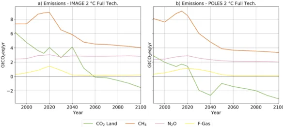
Although in terms of total greenhouse gas emissions the models show similar results, there are differences noticeable when decomposing emissions into separate greenhouse gas categories, as has been done in Figure 3. Looking first at the non-CO2 greenhouse gas

be reduced to zero (Figure 3). This is shown for both the IMAGE and POLES scenario and can in large part be explained that for several sources, only a constrained reduction potential has been identified, in particular from agriculture (e.g. for rice cultivation and animal husbandry) (Gernaat et al., 2015; Lucas et al., 2007). 8 _{N2O emissions hardly change over time, under}

both scenarios, and are quite similar for both models. CH4 emissions remain at around 3.5–

4.5 GtCO2eq after 2050, with the POLES scenario showing slightly lower projections. The

F-gas emissions reach zero, and are about the same for both models.

The land-use-related CO2 emissions are projected to decrease over time, reaching zero

under the POLES model by 2025, and for IMAGE by 2060. The land-use emission projections for the POLES scenarios remain about -2 GtCO2 after 2030, whereas for the IMAGE scenario

this level is not reached even by 2100. The 2010 emission levels are already lower in the POLES model, due to differences in the data sets being used by POLES and IMAGE to define the historical levels of emissions9_{, as explained in Section 3.1, and will be explained in more}

detail in Section 5.1.

Concluding, the scale of reduction potential in terms of CO2 emissions from land-use changes

and non-CO2 greenhouse gas emissions is lower compared to the emission reduction

potential in the energy sector for both models, as analysed below.

Figure 3. Global non-CO2 greenhouse gas emissions and land-use-related CO2 emissions,

under the 2 °C Full technology scenarios of IMAGE (panel a) and POLES (panel b).

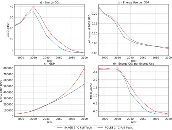
Significant reductions are achieved in both models in terms of energy- and industry-related CO2 emissions. A useful method for analysing the differences between models in terms of

energy- and industry-related CO2 emissions and emission reductions is the Kaya identity

(Kaya, 1989) that decomposes the emissions into four factors: population (Pop), per capita income (Pop/GDP), final energy (FE) intensity of economic production (FE/GDP), and carbon intensity of energy use (CO2/FE). Here, we combine the first two factors, population (Pop)

and per capita income (GDP/Pop), into the economic production (GDP). We also show primary energy demand instead of final energy use. Using the Kaya identities (Figure 4) we see that the lower energy- and industry-related CO2 emissions under the IMAGE scenario

(Figure 4a) are driven by a lower primary energy intensity of the economy (Figure 4b), (in

8 _{Including all potential reduction measures including management and structural changes would lead to a} higher reduction potential, as has been done in Frank et al. (2017).

9 _{Harmonising of the model projections implies that the starting point (2010) of the scenarios becomes the} same as the inventory data, but the emissions trend of the projections remains unchanged. See Chapter 6.

the second half of the century) a lower increase in GDP (Figure 4c) and lower carbon intensity of energy (Figure 4d).

Figure 4. Global Kaya indicators under the Full technology 2 °C scenarios of IMAGE and POLES. The panels show the energy- and industry-related CO2 emissions (panel a), primary

energy intensity of economic production (panel b), GDP (panel c) and carbon intensity of energy use (panel d).

Relating these emissions to other indicators shows that the reductions in energy- and

industry-related CO2 emissions under the Full technology IMAGE scenario are driven more by

improvements in energy efficiency than they are under the POLES scenario. It can be seen that, up to 2070, the IMAGE scenario has lower values for the energy per unit value of GDP and also lower values for energy-related CO2 emissions per unit of energy.

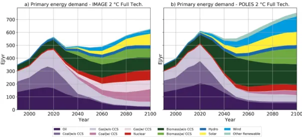
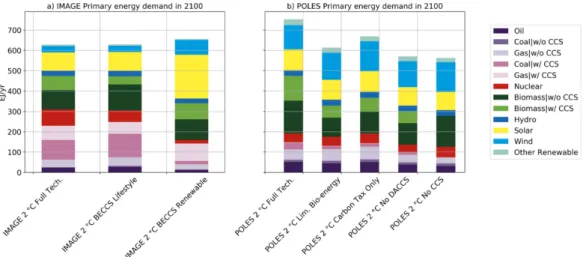
The lower energy intensity and GDP projections for the IMAGE scenario result in primary energy demand being lower compared to the POLES scenario, as is also illustrated in Figure 5. Emission reductions for the POLES scenario are driven to a lesser extent by energy efficiency improvements and more by decarbonisation. This becomes clear when looking in more detail at the primary energy demand.

The shares of renewables increase considerably from 2020 onward for the POLES scenario, especially when compared to the IMAGE scenario. Figure 5 gives a decomposition of primary energy demand for both these scenarios, showing a substitution of fossil primary energy for renewables, and a corresponding decline of carbon intensity of the economy after 2020 (as shown in Figure 4b).

In order to stay below 2 °C, both models convert the global energy system from one that is based almost completely on fossil fuels (as it is currently) to one in which renewable energy, nuclear power or CCS play an important role. The POLES scenario shows a larger increase in renewables use. In the IMAGE scenario the increase in nuclear power is larger and there is an increase in the use of CCS, both fossil and energy based. The overall use of

bio-energy is however lower for the IMAGE scenario compared to POLES, which assumes high bio-energy availability.

Figure 5. Global primary energy demand for the Full technology 2 °C scenarios of IMAGE (panel a) and POLES (panel b).

In the IMAGE scenario, the use of CCS starts already from 2025/2030 onwards, showing an increasing trend and leading to a large total share of CCS already by 2050, much larger compared to the POLES scenario. This large difference in the contribution of CCS is mainly caused by the cost-competitiveness of CCS versus other mitigation options in IMAGE. In addition, it is partly caused by the higher land-use-related CO2 emissions under the IMAGE

scenario and the more stringent climate target for the IMAGE scenario, which increases the need for greater reductions within the energy-system. This climate target leads to lower cumulative CO2 emissions for the 2010–2100 period under the IMAGE scenario, about 1000

GtCO2, compared to 1150 GtCO2 under the POLES scenario; from 2010 until 2100, CCS

technologies capture 770 and 480 GtCO2 in IMAGE and POLES, respectively. In addition, all

POLES scenarios consider CCS to be a technology that has not yet matured; the first CCS plants are only allowed to be installed in the 2030s and wider adoption just on the basis of costs happens only from 2050 onwards; as a result, the contribution of CCS in 2050 is lower in POLES. A more detailed analysis of the cumulative emissions is given in the Appendix A.

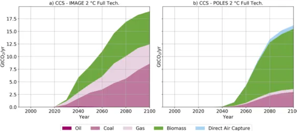
Both models also show a clear difference in contribution of CCS (Figure 6). IMAGE has a more even distribution of fossil fuels with CCS and BECCS than POLES. The large share of BECCS for POLES is a result of the cost-competitiveness of BECCS versus other options, despite high bio-energy prices because of biomass scarcity, and due to the high carbon price and capture rate of CCS being lower than 100%. In IMAGE, also fossil CCS remains

competitive given the increasing bio-energy prices because of biomass scarcity.

Finally, while in both models total biomass use increases over time, the models reach different levels overall. Biomass use in POLES increases by 2100 to a level (280 EJ/yr) close to the total global potential (300 EJ/yr, according to GLOBIOM). In IMAGE biomass use increases significantly up to 2040, then increases much more gradually afterwards to reach a lower level (165 EJ/yr); this level of biomass use is lower than the maximum potential (see 1.5 °C scenario, where IMAGE reaches levels similar to POLES).

Figure 6. Carbon captured per energy carrier, or by technology in the case of direct air capture, under the Full technology 2 °C scenarios of IMAGE (panel a) and POLES (panel b), for the energy carriers with CCS.

The 1.5 °C Full technology scenarios

Findings

 The Full technology 1.5 °C scenarios of both global models show that pathways

exist that limit global warming to below 1.5 °C by 2100, relying strongly on bio-energy and negative CO2 emission technologies.

 Global greenhouse gas emissions under the 1.5 °C scenarios reach net zero in the second half of the century, i.e. between 2050 and 2070, which is about 40 years earlier than under the 2 °C scenarios. Global emissions are reduced by 70% to 76% by 2050, from 1990 levels.

 Greenhouse gas emissions under the 1.5 °C scenarios of IMAGE and POLES

reach about -10 to -5 GtCO2eq/yr by 2100. This is within the range of Full

technology 1.5 °C scenarios from all global models in the SSP multi-model comparison study, albeit in the upper part of this range (Rogelj et al., 2018).

 Similar to the 2 °C scenarios, the IMAGE 1.5 °C scenario has greater energy

efficiency improvements and more CCS than the POLES 1.5 °C scenario. The POLES 2 °C scenario focuses more on decarbonisation of the energy system through more renewable energy supply.

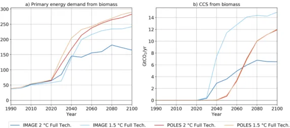
 Bio-energy use is significantly greater in the IMAGE 1.5 °C scenario, compared

to that in the 2 °C scenario, but it is almost the same in the POLES 1.5 °C scenario.

 There is significantly more deployment of BECCS in the IMAGE 1.5 °C scenario

than in the 2 °C scenario, whereas, in POLES, the deployment of BECCS is very similar in the 1.5 °C and 2 °C scenarios.

Results

Similar to the 2°C scenarios, in the 1.5 °C scenarios, the IMAGE and POLES models assume different climate constraints. The IMAGE model explores emission pathways for 1.5 °C assuming that radiative forcing reaches 1.9 W/m2 _{by 2100, whereas the POLES model}

explores emission pathways for achieving 1.5 °C by finding the cumulative anthropogenic CO2 emissions for the 2010–2100 period compatible with that temperature increase

(according to MAGICC) of around 550 GtCO2. This section again focuses on the Full

technology scenarios.

Figure 7 shows the greenhouse gas emission pathways for meeting 1.5 °C for the POLES and IMAGE model. It shows that POLES has slightly lower greenhouse gas emissions already in 2020. The emission reduction pathways for both models show a similar pattern, with emissions rapidly reducing after 2020, but the POLES scenario shows an even more rapid decline after 2020 and emissions go deeper in 2100 than they do for the IMAGE scenario.

Comparison with a range of cost-optimal SSP 1.9W/m2 _{scenarios run by other models (Rogelj}

et al., 2018) shows that both the POLES and IMAGE 1.5 °C scenarios are clearly within the range, over the whole period. However, specifically in 2050, both scenarios are more on the high end of the range (Figure 7). This is in contrast with the 2 °C scenarios of IMAGE and POLES, which show greenhouse gas emissions in 2050 at the lower end of the SSP 2.9 W/m2

scenario range. Under full technology assumptions the POLES and in particular IMAGE 1.5 °C scenarios lead to fewer negative emissions than other IAM full technology SSP 1.9W/m2

scenarios.

Figure 7 Global greenhouse gas emissions under the 1.5 °C Full technology scenarios of IMAGE and POLES, compared to a set of cost-optimal SSP 1.9 W/m2 _scenarios.

Under the 1.5 °C scenarios of IMAGE and POLES, global greenhouse gas emissions in 2050 are about 7 to 8 GtCO2eq lower than under their 2 °C scenarios, reaching 76% to 70%

reductions below 1990 levels, respectively. Global emissions under the 1.5 °C scenarios reach zero in the second half of the century, i.e. between 2060 and 2070, which is about 40 years earlier compared to under the 2 °C scenarios of IMAGE and POLES. Figure 7 shows that the time period (2060–2070) for which the zero emissions are reached are in the middle of the full range projected by all SSP 1.9 W/m2 _scenarios.

Looking at the pathways of individual greenhouse gases, we see that non-CO2 and

land-use-change-related CO2 emissions are similar under the 1.5 °C and 2 °C scenarios of both

models (Figure 8).

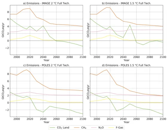
Figure 8. Global non-CO2 greenhouse gas emissions and land-use-change-related CO2

emissions in GtCO2eq/yr, under the 2 °C and 1.5 °C Full technology scenarios of IMAGE

(panel a and b) and POLES (panel c and d).

The sum of total non-CO2 greenhouse gas emissions and land-use-related CO2 emissions

expressed as CO2-equivalent emissions shows, for the IMAGE model, only a marginal

difference between the 1.5 °C and 2 °C scenarios, reaching about 5 and 7 GtCO2eq/yr,

respectively, by 2100 (see Table 4). In 2050, under the IMAGE 1.5 °C scenario, the land-use emissions are somewhat higher due to the expansion in bio-energy production. However, given the uncertainty about the timing, it is more useful to see the long-term trend. As such, the 2050 emission reduction for the 1.5 °C target is not structurally dissimilar from the one for the 2 °C target. For the POLES model, the total emissions, under the 1.5 °C and 2 °C emissions, reach much lower levels by 2100 (i.e. 0.5 and 2.5 GtCO2eq/yr), mainly due to

lower CH4 and land-use-related CO2 emissions. These remaining emissions need to be

compensated by more negative energy- and industry-related CO2 emissions (Figure 9a), in

particular under the 1.5 °C scenario, in order to reach negative greenhouse gas emission levels by 2100 (see Figure 6).