Regional Modelling of
Particulate Matter for
the Netherlands
Improved model system for Particulate Matter
This report is a technical background document about modelling of
Particulate Matter. For policy support, it is necessary to quantify the
relation between emissions, atmospheric conditions and concentrations
of air pollutants. In the Netherlands, two models are used for this purpose.
This document describes the two models and their recent developments
accomplished within the BOP research programme. The LOTOS-EUROS model
calculates air quality on a European scale and the OPS model focuses on the
Netherlands. The LOTOS-EUROS model was validated against observations and
further developed by including improved and new parameterisations for the
contribution of sea salt, mineral dust and biogenic secondary organic aerosol
to particulate matter. In addition, a coupling was realised between the global
air quality model TM5 and LOTOS-EUROS. Finally, the LOTOS-EUROS model and
the OPS model were tested in an intercomparison together with the unified
EMEP model for ammonium, nitrate, sulphate and fine primary particles.
This technical background report is a BOP publication produced under the
auspices of TNO.
The Netherlands Research Program on Particulate Matter (BOP) is a national
program on PM
10
and PM
2.5
. It is a framework of cooperation involving
the Energy Research Centre of the Netherlands (ECN), the Netherlands
Environmental Assessment Agency (PBL), the Environment and Safety Division
of the National Institute for Public Health and the Environment (RIVM) and
TNO Built Environment and Geosciences.
Technical background report BOP
Regional Modelling of Particulate
Matter for the Netherlands
M. Schaap, TNO; A.M.M. Manders, TNO; E.C.J. Hendriks, TNO; J.M. Cnossen, PBL;
A.J.S. Segers, TNO; H.A.C. Denier van der Gon, TNO; M. Jozwicka, TNO;
Regional Modelling of Particulate Matter for the Netherlands
This is a publication of the Netherlands Research Program on Particulate Matter Report 500099008
M. Schaap, A.M.M. Manders, E.C.J. Hendriks, J.M. Cnossen, A.J.S. Segers, H.A.C. Denier van der Gon, M. Jozwicka, F.J. Sauter, G.J.M. Velders, J. Matthijsen, P.J.H. Builtjes
Contact: karin.vandoremalen@pbl.nl ISSN: 1875-2322 (print) ISSN: 1875-2314 (on line) This is a publication in the series: BOP reports Project assistant: Karin van Doremalen English editing: Annemarieke Righart
Figure editing: PBL editing and production team Layout and design: RIVM editing and production team Cover design: Ed Buijsman (photographer: Sandsun) ECN Energy Research Centre of the Netherlands PBL Netherlands Environmental Assessment Agency TNO Built Environment and Geoscieces
RIVM National Institute for Public Health and the Environment
This study has been conducted under the auspices of the Netherlands Research Program on Particulate Matter (BOP), a national program on PM10 and PM2.5 funded by the Dutch Minis-try of Housing, Spatial Planning and the Environment (VROM).
Parts of this publication may be reproduced provided that reference is made to the source. A comprehensive reference to the report reads as ‘ Schaap M., Manders A.M.M., Hendriks E.C.J., Cnossen J.M., Segers A.J.S., Denier van der Gon H.A.C., Jozwicka M., Sauter F.J., Velders G.J.M., Matthijsen J., Builtjes P.J.H. (2009) Regional modelling of particulate matter for the Netherlands:
The complete publication, can be downloaded from the website www.pbl.nl, or a copy may be requested from reports@pbl.nl, citing the PBL publication number.
Netherlands Environmental Assessment Agency, (PBL) P.O. BOX 303, 3720 AH Bilthoven, the Netherlands; Tel: +31-30-274 274 5;
Fax: +31-30-274 4479; www.pbl.nl/en
This publication can be downloaded from the website www.pbl.nl/en. 5
Rapport in het kort
Dit rapport is een technisch achtergrond rapport over het modelleren van fijnstof. Voor het beleid is het noodzakelijk om de relatie tussen emissies, atmosferische omstandigheden en de concentraties van luchtverontreinigende stoffen te kwantificeren. In Nederland worden voor dit doel twee modellen gebruikt. Dit document beschrijft de twee modellen en recente ontwikkelingen die binnen het BOP onderzoeksprogramma bereikt zijn. LOTOS-EUROS berekent de luchtkwaliteit op Europese schaal terwijl OPS gericht is op Nederland. Het LOTOS-EUROS model is gevalideerd met metingen en verder ontwikkeld door de toevoeging van verbeterde en nieuwe routines voor het berekenen van de bijdrage van zeezout, bodemstof en biogene secundaire organische aërosolen aan fijnstof. Daarnaast is een koppeling gerealiseerd tussen het mondiale chemietransport model TM5 en LOTOS-EUROS. Tenslotte worden LOTOS-EUROS en OPS getest in vergelijking met het UNIFIED EMEP model voor ammonium, nitraat, sulfaat en primaire deeltjes.Contents 7
Contents
Rapport in het kort 5 Abstract 9 1 Introduction 11 1.1 Background 11 1.2 Goals and approach 11 1.3 Rational model choice 122
Model descriptions 13
2.1 The LOTOS-EUROS model 13 1.2 OPS 14 3 Base case 17 3.1 Methodology 17 3.2 Modelled distributions 17
3.3 Verification versus measurements 19 3.4 Discussion and conclusions 24
4
Sea salt 27 4.1 Introduction 27
4.2 Sea salt emission mechanisms 27 4.3 Particle size and density 28 4.4 New emission algorithm 28
4.5 Alternative scheme for dry deposition 29 4.6 Run description 29 4.7 Results 29 4.8 Verification 30 4.9 Discussion 33 4.10 Conclusions 36 5
Modelling of crustal matter 37
5.1 Emission module for windblown dust 37 5.2 Saharan desert dust 44
5.3 Resuspension due to traffic 44 5.4 Agricultural activities 54 5.5 Results 55 5.6 Verification 60 5.7 Discussion 62 5.8 Conclusions 63 6 Carbonaceous aerosol 65 6.1 Model development 65 6.2 Results and discussion 69
7
Model Intercomparison: LOTOSEUROS, EMEP and OPS 71 7.1 Introduction 71
7.2 Concentrations in the Netherlands 71
7.3 Source Receptor Matrices and 15% emission reductions 73 7.4 Relative reaction of PM to emission reductions 77 7.5 Conclusions 78
8
Outlook 81
Annex A New meteorological input
82
Annex B
Sea salt emission 83 Annex C Dry deposition
85
C.1 Zhang scheme 85 C.2 Discussion 86
Annex D Biogenic emission parameters
87
Annex E Boundary conditions from TM5
90
E.1 TM5 simulation :90
E.2 Coupling to LOTOS-EUROS 90 E.3 Results 90
E.4 Conclusion 91
Annex F Spatial distribution of PM components
93
References
Abstract 9
Particulate Matter (PM) causes adverse health effects. Therefore, it is subject to regulations. For policy support, it is necessary to quantify the relation between emissions, atmospheric conditions and concentrations of air pollutants; this is done by using models. Generally, models describe only about half of the PM10 concentration, which can be attributed to the known anthropogenic sources. Although sources and dispersion of the other half, like sea salt and mineral dust, are understood, in general terms, understanding by means of modelling is still rather poor. This forms a major handicap for source apportionment of PM concentrations. The Nether-lands Research Program on Particulate Matter (BOP) aims for a better understanding of PM by improving models especially with respect to sea salt and mineral dust.
This report is a background document which describes the two models used in the Netherlands and their recent develop-ments accomplished within the BOP research programme. The LOTOS-EUROS model, which calculates air quality on a European scale, and the OPS model, which focuses on the Netherlands, both belong to the main model instruments for policy support in the Netherlands. The LOTOS-EUROS model is further developed for PM by including (improved) param-eterisations for the contribution of sea salt, mineral dust and biogenic secondary organic aerosol. In addition, a coupling was realised between the global air quality model TM5 and LOTOS-EUROS. This coupling allowed for calculating the effects of global emission changes on European air quality. Finally, the LOTOS-EUROS model and the OPS model were tested in an intercomparison together with the EMEP model for ammonium, nitrate and sulphate, particles, which are chemically formed in the air from gases, and the fine primary particles, which are directly emitted into the air.
As a base case, the performance of the original operational LOTOS-EUROS version, without the new developments, was investigated and compared with observations within the Netherlands. The time correlation of total PM10 was reason-able, but absolute concentrations were underestimated, especially for the highest concentrations. Secondary inorganic aerosols were well represented, both in time and space. Elemental carbon and sea salt concentrations could not be validated well, and components such as mineral dust and secondary organic aerosol were not modelled. A simple bias correction was proposed to improve the modelling of total PM10.
Three adaptations were made to improve the model descrip-tion of sea salt:
The particle-size resolution was doubled 1.
The source function for the smallest sea salt particles was 2.
now according to Mårtensson (2003).
A new dry deposition scheme was introduced according to 3.
Zhang (2001).
The new sea salt parameterisation resulted in an improved representation of the model sea salt processes. However, sea salt concentrations which result from the improved parameterisation were an overestimation in comparison with European observations (between 50% and 100%). The mod-elled overestimation occurred especially at high wind speeds. Large uncertainties (by a factor of 10) in the sea salt source function formulations were likely to be the main cause of our overestimation.
Hereafter, mineral dust was included in the LOTOS-EUROS model as a new PM fraction. A description was made of three different mineral dust sources.
The emission of wind-blown dust (wind-induced abrasion) 4.
was included, taking soil texture, soil moisture and pre-cipitation into account. Dust which originates from large deserts outside the LOTOS-EUROS domain was included through coupling with the global model, TM5.
Resuspension of mineral dust due to traffic circulation was 5.
also included. The description includes the effects of pre-cipitation and a regional dependence in terms of climatic conditions on the basis of soil moisture information and observed PM concentrations.
A first effort was made to model the emission of mineral 6.
dust due to agricultural activity. The source function describes emission of mineral dust from agricultural land, based on the agricultural activity calendar and taking the effects of precipitation into account.
Furthermore, the modelling of biogenic volatile organic carbon emissions was improved. These emissions have an impact on the formation of secondary organic aerosol (SOA), for which the chemical formation scheme was also extended.
The intercomparison was based on modelled concentration levels and results from source receptor matrices (SRM) per model. Overall, the results of the LOTOS-EUROS model are closer too those of the EMEP model version 2.8 than those of the OPS model. The model intercomparison showed that
Abstract
per PM fraction model results were different for each model considered. The results from the models form a range, which can be seen as a margin of uncertainty when using models for policy support, provided that the models are equally fit.
The OPS model is currently used for calculating average annual concentrations of primary particulate matter (PPM) and the secondary inorganic aerosol (SIA) for the specific air quality situation in the Netherlands. OPS is not always suitable for scenarios studies on the effect of emission reductions of SO2, NOx and NH3, due to the absence of non-linear chemistry modelling. This is confirmed in this report by the SRM results, in particular, by those for NH3. The accuracy of the spatial dis-tribution of ammonium with OPS on a 1x1 km2 grid is limited due to the linear approach. Source-receptor data, generated with OPS, are reliable when NOx, SO2, and NH3 emissions are reduced proportionally and simultaneously.
The SRM results of LOTOS-EUROS, OPS and EMEP v2.8 could be generalised as follows. The relative reaction of the average particulate matter concentration in the Netherlands to 15% reduction in PPM2.5, NH3 and NOx was about the same for all three (several percents reduction). 15% emission reductions of SO2 lead to less than 1% reduction of PM. The reaction per kiloton emission change gave an impression of the effective-ness of emission changes. Reducing PPM2.5 was most effec-tive, naturally, followed by NH3, NOx and SO2. The reaction per kiloton of emission reduction, for all pollutants consid-ered, was largest in the Netherlands, followed by Belgium, Germany and France, and was the smallest in Great Britain.
Introduction 11
Background
1.1
While air quality in Europe has improved substantially over the past decades, air pollution still poses a significant threat to human health (EEA, 2007). Health effects of air pollution are dominated by particulate matter, both PM2.5 and PM10. Short-term exposure to PMx has frequently been associ-ated with increased human morbidity and mortality (e.g., Brunekreef and Holgate, 2002). Although the effects of long-term exposure to PM are much more uncertain than the effects of short-term exposure, they are believed to have a much greater effect on health loss (Dockery et al., 1993; Pope et al., 1995). Therefore, the European air quality standards currently focus on the total mass of the unspecified combined particles smaller than 10 μm in diameter (PM10), which cover the inhalable size fraction of PM. At present, many European countries, including the Netherlands, have problems attaining the daily limit value for PM10.
Mass and composition of PM10 tend to divide into two princi-pal groups: fine and coarse mode. The fine particles (typi-cally smaller than 2.5 microns) contain secondary inorganic aerosols (SIA), elemental carbon and organic material. The larger particles usually contain sea salt, earth crust materi-als and fugitive dust from roads and industries. To quantify the relation between emissions, atmospheric conditions and concentrations of air pollutants one depends on chem-istry transport models (CTMs). For a robust application of a regional CTM in policy support studies such as the evalua-tion of mitigaevalua-tion strategies, it is important that the model can represent the air pollutant concentration and the most important processes affecting the concentration in a satisfac-tory way. However, for particulate matter the current CTMs underestimate the PM10 concentrations by about 40 to 50%. This so-called non-modelled fraction comprises a number of PM components: sea salt, crustal material, secondary organic material and water. To gain more insight in the variability of the PM10 concentrations and the mechanisms that lead to concentrations above the daily mean threshold of 50 μg/m3 one needs to incorporate these components in the model. This report describes the effort to develop or incorporate a modelling framework for sea salt, dust and secondary organic aerosol for use in the CTM LOTOS-EUROS.
Goals and approach
1.2
This report aims to provide a technical background docu-ment to the modelling work performed in the project of the Netherlands Research Program on Particulate Matter (BOP). To put the work into the perspective of the BOP programme, we describe several research questions that contribute to the main purpose of the programme. Each research ques-tion was translated into a quesques-tion relating to modelling (placed in italics). The motivation and the approaches used for answering these questions are described below each research question. The methodologies for answering the research questions are described in this report. The use of the LOTOS-EUROS model to answer these policy and science related questions is described in the main thematic reports of the project.
What are the mechanisms that lead to an exceedance of the daily limit value and which sources and/or components contribute the most to these high pollution days? Can we use modelled particulate matter distributions to address exceedance days?
Chemistry transport models provide a relation between emissions, atmospheric conditions and concentrations of air pollutants. However, for PM10 CTMs underestimate the total concentrations. First we examined the perform-ance of LOTOS-EUROS for PM10 by a comparison between modelled and measured PM10 concentrations in the Netherlands. To detail the model performance, making a comparison between the PM components was manda-tory. Hence, we performed the analysis to the furthest extent possible, which is described in Chapter 3.
What is the contribution of sea salt to the PM10 and PM2.5 concentration on an annual basis and on days with limit value exceedances? How well does the model perform for sea salt?How sensitive are the modelled sea salt contributions to the choice of emission and dry deposition parameterisation?
Sea salt is modelled in all models used in the Netherlands. However, models use different methodologies for the emission parameterisation. These different modules may have a large impact on the modelled distribution. Here, we update the model description to the combination of emission parameterisations that is considered to be state-of-the-art. In addition, the model results for sea salt have not been extensively validated for both Dutch and European conditions. For the Netherlands, validation and
assessments of sea salt concentrations have relied largely on chloride measurements which are not well defined. Therefore, the BOP measurements and the efforts to compile foreign data provide the first opportunity for a more extensive validation. Furthermore, the coarse mode sea salt distribution is sensitive to the parameteri-sation used for the dry deposition, which largely deter-mines the transport distance. We tested the impact of a scheme based on theory to compare the results to the empirical approach that was used up to now. This work is described in Chapter 4.
What is the contribution of soil dust to the PM10 and PM2.5 concentration on an annual basis and on days with limit value exceedances? How can we model crustal matter emissions and to which extent can we estimate the source strength of this component?
Crustal material or soil particles typically contribute between 5 and 20% to the ambient PM10 mass. Despite the importance of crustal material in total PM10 mass, the sources are still scarcely understood and not (well) repre-sented in emission inventories or air quality models. Here we aimed to develop a methodology for checking first-order estimates of the various source strengths in Europe and in the Netherlands, in particular. For this purpose, we implemented simple and therefore transparent emission functions for wind erosion, (re-)suspension by traffic and agricultural land management. Furthermore, we included boundary conditions for desert dust from the global TM5 model. A first assessment of the model performance is also given in Chapter 5.
What is the contribution of carbonaceous material to the PM10 and PM2.5 concentration on an annual basis and on days with limit value exceedances? How can we model the formation of organic material in the atmosphere?
Chemistry transport models underestimate the concen-trations of carbonaceous material. Previous studies have concluded that the emissions of elemental carbon (EC) and organic carbon (OC) are probably underestimated. In addition to primary EC and OC, secondary organic aerosol may contribute significantly to the observed OC levels. The formation of secondary organic aerosols (SOAs) is not represented in LOTOS-EUROS. Several schemes have been documented in literature. However, current under-standing is so uncertain that we have incorporated a scheme that is flexible and can easily be extended in the future. The chosen approach is described in Chapter 6.
What is the contribution of non-European sources to PM levels in the Netherlands? What is the impact of using boundary conditions from a global modelling system?
Dutch levels of PM may be affected to some extent by sources from outside the model domain. Current practice incorporates an estimated 0.9 μg/m3 into the annual average PM10 concentration. For sea salt, dust and ozone, the impact is estimated to be non-negligible and we tested the use of a global CTM to provide the bound-ary conditions for LOTOS-EUROS. In Chapter 7, we will demonstrate that the model is capable of using boundary conditions from TM5.
Note that the model development with BOP is not performed based on the BOP measurement programme as both activities are performed simultaneously. Moreover, the observation database was not available when this report was printed. Hence, all model results shown in this report are for the year 2005. Comparison of the model results to the BOP measure-ments will be shown in thematic reports.
Rational model choice
1.3
In the Netherlands, two models are used for policy support. The first is the OPS model, developed by the Netherlands Environmental Assessment Agency (PBL). The second model is the LOTOS-EUROS model developed by TNO Built Environ-ment and Geosciences and the National Insitute for Public Health and the Environment (RIVM). For the BOP project, LOTOS-EUROS was chosen over OPS to be used as the central model for development. The first reason for this is that it has full photochemistry incorporated which is necessary to address the secondary aerosols properly. Furthermore, the model incorporates a larger domain and performs calcula-tions on an hourly basis using analysed meteorology, enabling a more extensive comparison with observations. Finally, LOTOS-EUROS is well documented with respect to its per-formance in comparison to other European models.
Considering the different model approaches in LOTOS-EUROS and OPS, a variability of the results between the models is expected. Therefore, an assessment was performed to find out the most important differences in the results of the models in a policy oriented application (Chapter 8). In addi-tion to the Dutch models, the unified model from the Euro-pean Monitoring and Evaluation Programme (EMEP) is also incorporated in the comparison as this model is used within the convention on trans-boundary air pollution
To guarantee that OPS also benefits from the BOP project, all developed parameterisations within this report will be made available to the developers of OPS.
Model descriptions 13
The LOTOS-EUROS model
2.1
The LOTOS-EUROS model is an operational air quality and chemical transport model of intermediate complexity focused on modelling the composition of the lower part of the troposphere. The model is used for calculating air pollutant concentrations and depositions on a regional scale [Schaap et al., 2008]. The LOTOS-EUROS model has been frequently used in policy support studies for the Netherlands, Germany and Europe. Furthermore, the model has been developed and used in a large number of European research projects. The model describes the processes of emission, transport, chemical conversion and dry and wet deposition. The LOTOS-EUROS model can be characterised as an Eulerian model in which all processes are solved at an evenly distributed grid. Up to now, the LOTOS-EUROS modelling system could be applied for the following components:
Oxidants: O3, VOC’s, NOx, HNO3, etc
Secondary inorganic aerosol (SIA): SO4, NO3, NH4
Secondary organic aerosol (SOA) from terpenes
Primary aerosol:
PPM2.5, PPM10-2.5, Black Carbon (BC), sea salt.
Heavy metals: Cd, Pb and other non-volatile metals POP’s: BAP, etc.
Particulate Matter in LOTOS-EUROS is modelled as the sum of the individual components as these components have different origins and atmospheric behaviour. At the start of the BOP project, PM10 is defined as the sum of the secondary inorganic components, the primary emitted particles and sea salt:
PM10 = SO4 + NO3 + NH4 + PPM2.5 + PPM2.5-10 + EC + SS
Considering that PM2.5 is part of PM10, it is calculated similarly but the coarse primary and sea salt particles are excluded from the summation:
PM2.5 = SO4 + NO3 + NH4 + PPM2.5 + EC+ SSfine
As noted before, secondary organic aerosols and crustal matter were not included in LOTOS-EUROS at the start of the project and their contributions should be added when they become available in LOTOS-EUROS.
A description of the model characteristics is given below.
Domain
The master domain of LOTOS-EUROS is bound at 35° and 70° North and 10° West and 60° East. The projection is a normal longitude−latitude and the standard grid resolution is 0.50° longitude x 0.25° latitude, approximately 25x25 kilometres. The model code is structured such that zooming (up to a factor of 8) is possible. Currently, there are three vertical dynamic layers and an optional surface layer. The model extends in a vertical direction for 3.5 kilometres above sea level. Note that, in this study, we added an extra layer of 3.5 to 5 kilometres. The lowest dynamic layer is the mixing layer, followed by two reservoir layers. The height of the mixing layer is part of the diagnostic meteorological input data. The heights of the reservoir layers are determined by the differ-ence between the mixing layer height and 3.5 kilometres. Both reservoir layers are equally thick with a minimum of 50 metres. In some cases when the mixing layer extends near or above 3500 metres the top of the model exceeds the 3500 metres according to the abovementioned description. Simula-tions were performed with the optional surface layer with a fixed depth of 25 metres. Hence, this layer is always part of the dynamic mixing layer. For output purposes, the concen-trations at measuring height (usually 3.6 m) are diagnosed by assuming that the flux is constant with height and equal to the deposition velocity times the concentration at height z.
Transport
The transport consists of advection in 3 dimensions, horizon-tal and vertical diffusion, and entrainment or detrainment. The advection is driven by meteorological field (u,v) input, every three hours. The vertical wind speed w is calculated by the model to be a result of the divergence of the horizontal wind fields. The improved and highly accurate, monotonic advection scheme developed by Walcek (2000) is used to solve the system. The number of steps within the advection scheme is chosen in such a way that the courant restriction is fulfilled. Entrainment is caused by the growth of the mixing layer during the day. Each hour, the vertical structure of the model is adjusted to the new mixing layer depth. After the new structure is set, the pollutant concentrations are redis-tributed by using linear interpolation.
The horizontal diffusion is described with a horizontal eddy diffusion coefficient following the approach by Liu and Durran (1977). Vertical diffusion is described using the standard Kz theory. Vertical exchange is calculated by employing the new integral scheme by Yamartino et al. (2004).
Chemistry
The LOTOS-EUROS model contains two chemical mechanisms, the TNO CBM-IV scheme (Schaap et al., 2005) and the CBM-IV by Adelman (1999). In this study we used the TNO CBM-IV scheme which is a modified version of the original CBM-IV (Whitten et al., 1980). The scheme includes 28 substances and 66 reactions, including 12 photolytic reactions. Compared to the original scheme steady state approximations were used to reduce the number of reactions. In addition, reaction rates have been updated regularly. The mechanism was tested against the results of an intercomparison presented by Poppe et al. (1996) and found to be in good agreement with the results presented for the other mechanisms. Aerosol chemis-try is represented by using ISORROPIA (Nenes et al., 1999).
Dry and wet deposition
The dry deposition in LOTOS-EUROS is parameterised fol-lowing the well-known resistance approach. The deposition speed is described as the reciprocal sum of three resistances: the aerodynamic resistance, the laminar layer resistance and the surface resistance. The aerodynamic resistance is depend-ent on atmospheric stability. The relevant stability parameters (u*, L and Kz) are calculated by using standard similarity theory profiles.
The laminar layer resistance and the surface resistances for acidifying components and particles are described following the EDACS system (Erisman et al., 1994).
Below-cloud scavenging is described by using simple scaveng-ing coefficients for gases (Schaap et al., 2005) and followscaveng-ing Simpson et al. (2003) for particles. In-cloud scavenging is neglected due to the limited information on clouds. Neglect-ing in-cloud scavengNeglect-ing results in wet deposition fluxes that are too low, but it has a very limited influence on ground level concentrations (see Schaap et al., 2004a).
Meteorological data
The LOTOS-EUROS system in its standard version is driven by 3-hourly meteorological data. These include three-dimen-sional fields for wind direction, wind speed, temperature, humidity and density, substantiated by two-dimensional gridded fields of mixing layer height, precipitation rates, cloud cover and several boundary layer and surface variables. The standard meteorological data for Europe are produced at the Free University of Berlin employing a diagnostic mete-orological analysis system based on an optimum interpola-tion procedure on isentropic surfaces. The system utilises all available synoptic surface and upper air data (Kerschbaumer and Reimer, 2003). Also, as was done for this study, meteoro-logical data obtained from ECMWF can be used to force the model.
Emissions
The anthropogenic emissions used in this study are a com-bination of the TNO emission database (Visschedijk and Denier van der Gon et al., 2005) and the Clean Air For Europe (CAFE) baseline emissions for 2000. For each source category and each country, we scaled the country totals of the TNO emission database to those of the CAFE baseline emissions. Elemental carbon (EC) emissions were derived from (and
subtracted from) the primary PM2.5 (PPM2.5) emissions follow-ing Schaap et al. (2004b). Hence, we used the official emis-sion totals as used within the protocol of long-ange trans-boundary air pollution (LRTAP), but we benefited from the higher resolution of the TNO emission database (0.25°x0.125° longitude−latitude). The annual emission totals were broken down to hourly emission estimates by using time factors for the emissions strength variation over the months, the days of the week and the hours of the day (Builtjes et al., 2003).
In LOTOS-EUROS, biogenic isoprene emissions were calcu-lated following Veldt (1991) by using the actual meteorologi-cal data. In addition, sea salt emissions were parameterised following Monahan et al. (1986) from the wind speed at ten-metre heights.
Boundary conditions
The lateral boundary conditions used in this study were obtained by a simulation of the LOTOS-EUROS model with its full domain. Model top boundary concentrations were set to 0.8 ug/m3 for sulphate, and ammonium was set to neutralise the sulphate. Other aerosol substances were set to zero. Ozone concentrations were obtained from Logan (1999).
Use of the LOTOS-EUROS model
The LOTOS-EUROS model is used for air quality studies at several institutes in the Netherlands. Presently, the LOTOS-EUROS consortium consists of TNO, PBL, RIVM and KNMI. Furthermore, researchers at several universities have access to the model. In the last two years, the model has been used to perform air quality studies for VROM, PBL, EEA, UBA Germany and the EU DG Environment. Scientific studies have been performed to address aerosol nitrate (Schaap et al., 2004a; 2007), black carbon (2004b; 2007), heavy metals (Denier van der Gon et al., 2008), PM10 (Van Zelm et al., 2008); Van de Kassteele et al., 2007), ozone (Vautard et al., 2006) and POP’s (Hollander et al., 2007). The model has frequently par-ticpated in international model comparisons aimed at ozone (Van Loon et al., 2007; Hass et al., 200x), PM (Cuvelier et al., 2007; Hass et al., 200x; Stern et al., 2008; Schaap et al., 2008) and source Receptor Matrices (Thunis et al., 2008). Recently, data assimilation techniques have been used to perform a combined assessment of the air pollution levels using the model and observational data (e.g. Van Loon et al., 2001; Denby et al., 2008; Barbu et al., 2008). A new direction is the use of satellite data in combination with these data assimila-tion techniques (e.g. Koelemeijer et al., 2006; Timmermans et al., 2008).
OPS
1.2
The OPS model is used for calculating time averaged con-centrations and depositions on a local to regional scale from European emissions to the atmosphere [Van Jaarsveld, 2004]. OPS model results are used in combination with air quality measurements for assessment of air pollution in the Neth-erlands [e.g. Velders et al., 2008]. The model describes the processes of emission, transport, chemical conversion and dry and wet deposition. The OPS model is a universal air quality dispersion model and is a fit for those substances for which
Model descriptions 15
the atmospheric loss processes can be described as first-order loss reactions. Ozone is therefore excluded. The OPS model can be characterised as a Lagrangian model in which the transport equations are solved analytically. Contribu-tions from the various sources are calculated independent of each other by using backward trajectories; local dispersion is introduced via a Gaussian plume formulation. Dry deposition, wet deposition and chemical conversion are incorporated as first-order processes and independent of concentrations of other substances. The only exception is the dry deposition of NH3 and SO2, which are mutually dependent.
The basic meteorological data needed by the model (wind direction and velocity, temperature, solar radiation and pre-cipitation) are taken from 16 stations of national meteorologi-cal network in the Netherlands. This includes also data from the 200 meter meteorological tower at Cabauw. On the basis of these data meteorological statistics are derived with a specific pre-processor for six regions within the Netherlands. The model determines for every receptor point specific dis-persion properties for every receptor point by interpolation of the regional data and depending on terrain roughness. The operational OPS model calculates long-term average (yearly) concentrations and depositions. A short-term version of the model is available.
Validation
OPS model results agree with air pollution concentrations (trends and spatial distribution) as measured by the Dutch national air quality monitoring network [LML, 2008] over the past 10 to 20 years. This is especially true, on a yearly basis, for the following substances: sulphur dioxide (SO2) and particu-late sulphate (SO4), nitrogen oxides (NOx) and particulate nitrate (NO3), ammonia (NH3) and particulate ammonium (NH4) (with r = 0.88 to 0.93 for SO2 and NOx) [Van Jaarsveld, 1989, 1995 and 2004; Asman and Van Jaarsveld, 1990].
Use of the OPS model
The OPS model is widely used for air quality studies in the Netherlands [see e.g. Van Jaarsveld, 2004 and references therein]. The model has also been adapted (Mensink and Janssen, 1996) to be used in Flanders, for Belgian air quality assessments. Source receptor matrices, calculated by the OPS model, have served as input for a Dutch version of the GAINS model (Wagner et al., 2007), GAINS-NL (Aben et al., 2005). GAINS-NL combines the high resolution of the OPS model with the integrated approach of the GAINS model.
OPS differs from LOTOS-EUROS (LE)
There are several differences between the OPS and LE models.
Dispersion: the OPS model treats dispersion in a Lagrang-1.
ian way and includes a Gaussian plume formulation for local dispersion, whereas the LE model applies a Eulerian approach on a grid. The differences have consequences for the final particulate matter results. Results following the OPS model approach are not better or worse, a priori, then when following an Eulerian approach. Lagrangian models are usually computationally more demanding. The dispersion of point source emissions, especially on the scale of the (Eulerian) grid size, are better described by
using a Lagrangian approach. Primary particulate matter is emitted from point sources (e.g. chimneys or car exhausts) as well as in a diffuse manner (e.g. by sea salt).
Resolution: the time resolution of the operational OPS 2.
model is one year, whereas the LE model calculates concentration levels with time steps of half an hour. The OPS model therefore does not describe the day-to-day behaviour of particulate matter. It is important to under-stand the behaviour of particulate matter, for instance, regarding compliance to the limit value of 50 μg/m3 for daily average PM10 concentrations.
The spatial resolution of both models is also different. The 3.
OPS model calculates concentration levels for receptor points which are converted to gridded concentrations on a 5×5 km2 or 1×1 km2 resolution, depending on the input resolution of the gridded emissions (e.g. NH3 emissions are gridded with a resolution of 0.5×0.5 km2). LE has a standard resolution of approximately 25×25 km2, but can zoom in with a resolution of about 5×5 km2. The LE model describes air-quality parameters in four layers for the lower troposphere .
Chemistry: the OPS model does not include complex 4.
chemical reactions, although (semi) first-order reactions for modelling some important chemical conversions are included. The LE model, however, is designed to calculate long-term ozone concentrations and therefore carries extensive oxidant and aerosol chemistry for the tropo-sphere. It describes the non-linear behaviour of oxidants and aerosols.
Boundary and initial conditions: the OPS model does not 5.
apply boundary conditions to particulate matter calcula-tions nor does it set initial condicalcula-tions. The LE model uses fixed boundary conditions at the sides and the top of the domain, of around 3.5 kilometres. These conditions may vary in time and place, as if the LE model were nested into a hemispheric or global model. There is however no dynamic interaction between boundary conditions and the model.
Although other differences exist between the OPS and LE models in the description of other processes such as wet and dry deposition, basically, they are not different.
Base case 17
To quantify the relation between emissions, atmospheric con-ditions and concentrations of air pollutants, one depends on chemistry transport models (CTMs). For a robust application of a regional CTM, it is important that the model effectively can represent the concentration of air pollutants and the most important processes affecting the concentration. This chapter illustrates that chemistry transport models, including LOTOS-EUROS, underestimate the ambient PM10 concentra-tions. In doing so, we describe the status of LOTOS-EUROS before the implementation of new parametersations in the BOP programme. This chapter also shows the annual mean distributions as calculated by the model and examines the performance of the LOTOS-EUROS model for PM10 by com-paring the modelled and measured concentrations for the Netherlands. To discuss the model performance in detail, a comparison between the individual PM components is neces-sary. Section 3.1 describes the simulation set-up and meas-urement data for the year under study, 2005. The modelled annual average distributions are presented in Section 3.2 and compared to observations in Section 3.3. To examine the modelled variability in PM10 concentrations and the possibility of having to perform a bias correction, we have incorporated more data by extending the analysis to include the period from 2004 to 2006. The model results are discussed in Section 3.4.
Methodology
3.1
Run description 3.1.1
We performed a simulation for a European domain, bound at 35° and 70° North and 10° West and 40° East. The grid resolu-tion for this domain was 0.50° longitude x 0.25° latitude, i.e. approximately 25x25 kilometres over the Netherlands. Using a one-way zoom option, a high resolution simulation was obtained for the Netherlands and its direct surroundings, with an increase in resolution by a factor of four. The model was forced by using ECMWF meteorology and anthropogenic emissions (TNO-GEMS emission database). Natural sea salt (SS) emissions were calculated by the model, using Na as a tracer. Hourly concentrations of all particulate components were stored. The PM10 concentrations were diagnosed as the sum of the separate model components:
PM10 = SO4 + NO3 + NH4 + PPM10 + SS,
with PPM10 = PPM2.5 + PPMcoarse + EC
From the primary PM2.5 (PPM2.5) the elemental carbon (EC) component was also calculated, following Schaap et al. (2004b). Crustal matter (CM) and secondary organic aerosols (SOAs) were not yet incorporated in the base model version, because of a lack of solid knowledge both on emission strengths for CM and formation routes for SOA.
Monitoring data 3.1.2
To verify the modelled concentrations for the Netherlands, we used monitoring data from the national air quality network as operated by the RIVM (Beijk et al., 2007a). The network includes 15 rural stations for PM10 (see Figure 3.1). All data were corrected for sampling losses by using the standard procedures of the RIVM (Beijk et al., 2007b). For the evaluation of LOTOS-EUROS, only rural background stations were used, since the resolution of LOTOS-EUROS is not high enough to produce road-level results. Furthermore, second-ary inorganic aerosol concentrations were obtained for six rural locations. Finally, we used black smoke measurements to assess the model performance for EC. EC concentration data were estimated by using the empirical relation between black smoke and EC as determined by Schaap and Denier van der Gon (2007). As different analysing procedures for EC systematically yield different levels (by up to a factor of 2) (Ten Brink et al., 2004), the information was mainly used for assessing the temporal performance of the model.
The results of the model at the abovementioned stations were evaluated for PM10 by using a range of statistical param-eters. These are: average, root mean square error, residue, standard deviation of error, correlation, hit rate, hit ratio, and percentage of correct alarm (in the concentration interval of 50 to 200 μg/m3).
Modelled distributions
3.2
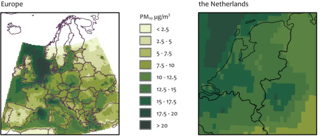
In this section, we present the modelled concentration data for PM10 and its components. In Figure 3.2, we present the modelled annual mean PM10 distribution for Europe as a whole and for the Netherlands, for 2005. The European domain shows maxima over the Benelux, Poland and the Po Valley (Italy). In these areas, the modelled concentrations exceeded 15 µg/m3. Similarly, large cities or agglomerations are recog-nisable with similar concentrations. Concentrations of 7.5 to 15 µg/m3 were found for a band over northwestern Europe, central and southeastern Europe. In general, the modelled
PM10 concentrations declined from Central Europe to northern Scandinavia and towards the Iberian Peninsula.
The modelled concentrations for the Netherlands showed levels between 10 and 20 µg/m3. The lowest concentrations were modelled for the province of Groningen. Concentrations between 14 and 18 µg/m3 were calculated for the populated western part of the Netherlands and for the river area stretching towards the Ruhr Area in Germany. Note that the modelled concentrations for the Belgian cities were (mod-elled to be) higher than those for the Netherlands. Minimum
concentrations over the zoom area were calculated over the forest regions of the Ardennes and Germany, south-east of the Ruhr Area.
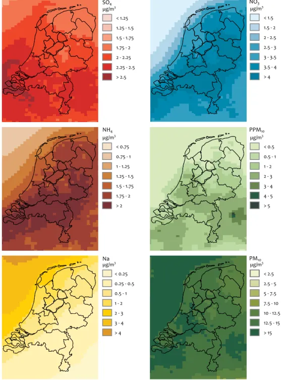
The annual average distributions of the modelled compo-nents are shown in Figure 3.3. Comparison of the distribution showed that each component had a specific distribution over the Netherlands. Sulphate contributed 1.7 to 2.2 µg/m3 to the PM10 concentration. It had a relatively even distribution over the Netherlands with maximum concentrations over a band connecting the Ruhr Area and the southern part of the
LML stations in the Netherlands used in the verification of the modelled PM10 distribution. All stations have been indicated by station number.
Figure 3.1 934 929 918 818 738 722 633 631 538 444 437 318 235 230 133 131
LML stations in the Netherlands
Base case 19
Netherlands. Maximum concentrations occurred above the sea because of combined local emissions by international shipping and an efficient above-sea conversion to sulphate. Nitrate was the largest contributor (> 3 µg/m3) to PM
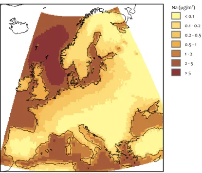
10 in the model. The distribution had a strong continental signature. The reason for this was the ammonium nitrate in the model, a semi-volatile component. High concentrations of ammonia are needed to stabilise the ammonium nitrate, especially in summer. The distribution showed characteristics of the ammonia emission strength. Ammonium neutralises both sulphate and nitrate and therefore shows features of both anions. The primary PM10 concentration peaked at locations with the highest emission levels, that is, the cities in the Randstad and around large sources, such as the Rotterdam harbour and Corus. At these locations, the primary material exceeded the contribution of nitrate. Finally, the sodium content of sea salt is shown. Sodium showed a large gradient from open sea to locations further inland. The reason for this is the short lifespan of coarse mode aerosol, in which most of the sea salt is found, causing a limited transport distance inland. Figure 3.3 also shows the total PM10 again, but with a different colour scale highlighting the gradients within the country.
Verification versus measurements
3.3
To assess the performance of the model we compared its results to measurements of the Dutch national monitoring network, LML. As both PM10 and PM2.5 are modelled as the sum of individual model components, we addressed the com-ponents first. Thereafter, the PM10 total mass was addressed. Unfortunately, there are no PM2.5 data available for 2005 in the Netherlands. Finally, we addressed the model perform-ance as a function of PM10 mass concentration.
PM
3.3.1 10 Components
We paired the daily observations available from the LML to modelled concentrations. Before we evaluated the total PM10 concentration, we examined the components. Table 3.1
shows the mean and standard deviations from observed and modelled concentrations at the monitoring locations. The cor-relation between observations and model and the root mean square error (RMSE) are also shown. The data represent the average values for the measurement locations. Note that the observations on individual components were only available at a small number of stations.
For the modelled secondary inorganic components, the annual mean concentrations were close to those from the observations. The contribution of nitrate (NO3) was slightly overestimated by LOTOS-EUROS, but the variability in the daily mean concentrations was quite comparable with the observations. Sulphate (SO4) was overestimated or underes-timated depending on the site, and the modelled variability was slightly too small. Ammonium aerosol (NH4) was compa-rable to or slightly above the observed concentrations, with variability in accordance with the observations. The temporal correlation for nitrate was slightly better than for sulphate, which may have been due to the generally higher concentra-tions of nitrate (and the associated lower amount of data below the detection limit).
The comparison for sea salt was hampered by the amount of available measurement data. The measurement strategy aimed at secondary inorganic aerosols also includes an analy-sis of the chloride (Cl) content. However, the measurement is not ideal as the available Cl observations only approximately cover the PM3 fraction, not the PM10 fraction. Moreover, Cl is lost because of chemical reactions in the atmosphere. This means that the sea salt estimate from chloride alone would be lower than the real and, therefore, also the modelled concentrations, as was indeed the case. Moreover, many of the observed concentrations were below the detection limit. Consequently, we interpreted the correlation coefficient (R=0.54) given in Table 3.1 as a lower limit. Comparison with a single month of observed Na concentrations available for 2005, showed a fairly good correspondence, although LOTOS-EUROS seemed to overestimate the concentrations for that
Modelled annual mean PM10 concentration (μg/m3) for Europe (left) and the Netherlands (right)..
Figure 3.2 Annual mean modelled concentration
Europe PM10 µg/m3 < 2.5 2.5 - 5 5 - 7.5 7.5 - 10 10 - 12.5 12.5 - 15 15 - 17.5 17.5 - 20 > 20 the Netherlands
month. For a more detailed discussion on sea salt we refer to Chapter 4.
Primary PM10 and PM2.5 are not observed. They were modelled as direct emissions from emission databases and are pre-sented in Table 3.1 to complete the overview of modelled con-centrations. Their composition is a mixture of further unspeci-fied substances, except for black carbon which was estimated based on an earlier study. However, black (or elemental)
carbon is not routinely measured in the monitoring network. We compared the black carbon model results with black smoke observations. Black smoke is in fact not identical to black carbon but can be used as a proxy for elemental carbon, with a conversion factor which depends on the individual station because of regional differences in aerosol character-istics and differences in station type (Schaap and Denier van der Gon, 2007). By using the linear relation between black smoke (BS) and EC by Schaap and Denier van der Gon (2007),
Annual mean distributions (µg/m3) of the model components sulphate (SO4), nitrate (NO3), ammonium (NH4),
primary PM10 (PPM10) and sea salt sodium (Na). For completeness the distribution of PM10 is also shown.
Figure 3.3 Annual mean distributions of model components
NO3 PM10 µg/m3 < 2.5 2.5 - 5 5 - 7.5 7.5 - 10 10 - 12.5 12.5 - 15 > 15 µg/m3 < 0.25 0.25 - 0.5 0.5 - 1 1 - 2 2 - 3 3 - 4 > 4 µg/m3 < 0.5 0.5 - 1 1 - 2 2 - 3 3 - 4 4 - 5 > 5 µg/m3 < 0.75 0.75 - 1 1 - 1.25 1.25 - 1.5 1.5 - 1.75 1.75 - 2 > 2 µg/m3 < 1.5 1.5 - 2 2 - 2.5 2.5 - 3 3 - 3.5 3.5 - 4 > 4 SO4 µg/m3 < 1.25 1.25 - 1.5 1.5 - 1.75 1.75 - 2 2 - 2.25 2.25 - 2.5 > 2.5 NH4 PPM10 Na
Base case 21
we estimated the annual mean EC concentration (from BS = 6.12) at the Dutch sites to be (0.056 * 6.12 + 0.12 =) 0.46. The modelled value was about twice as higher, which is within the uncertainty of the measurements on which the relation was based (Ten Brink et al., 2004). For a detailed discussion on EC and OC measurement techniques we refer to the thematic report on carbonaceous particles. The temporal correlation between the estimated EC or BS and the modelled values is, however, evident.
In short, the performance of the LOTOS-EUROS system was satisfactory for secondary inorganic aerosol. We could not draw strong conclusions for sea salt nor for black carbon. Their concentrations were not unrealistic and the temporal variation was well represented. Earlier comparisons against data from other countries have confirmed these findings (Schaap et al., 2008).
Below, we compared the total particulate mass to the PM10 measurements, to assess in how far we could explain the observed PM10 concentrations by using LOTOS-EUROS.
Bias correction for PM
3.3.2 10
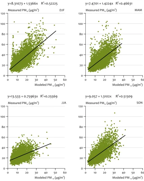
The modelled PM10 concentration is the sum of the individual model components. Since LOTOS-EUROS does not include all PM sources and components, the model underestimated observed PM10 levels. This is a common feature of present day CTMs (Yu et al., 2008, Stern et al., 2008). As for the model components, the temporal correlation (R=0.68) for PM10 is quite reasonable. To use LOTOS-EUROS for assessing the variability in total PM10, the missing fraction had to be compensated for. On average, LOTOS-EUROS underestimated the observed PM10 by 46 % or 11.7 µg/m3. In Figure 3.4, we explored the bias as a function of season, for 2004 to 2006. In the Figure, we compared all observations for all sites to the modelled value. The scatter plots indicate that the behaviour in summer differed from the other three seasons. In summer, the variability in modelled PM10 was lower than in the other seasons and the slope of the fit between the data was lower than 1. Hence, we used the seasonal fit parameters for esti-mating the bias corrected values:
PM10biascor = 1.54 * PM10 + 8.1 Winter (DJF)
PM10biascor = 1.42 * PM10 + 7.5 Spring (MAM)
PM10biascor = 0.76 * PM10 + 13.5 Summer (JJA)
PM10biascor = 1.31 * PM10 + 9.1 Autumn (SON)
We neglected the variation between stations and parts of the country to keep the procedure simple and transparent.
We assessed the quality of the LOTOS-EUROS model, includ-ing a bias correction, compared to the observations. Table 3.2 contains the values of the most important statistical parameters which are generally used to evaluate the perform-ance of models. We also included the persistence model for comparison. The persistance model is the model in which the modelled concentration simply is the observed concentration of the day before. The mean of the bias-corrected LOTOS-EUROS simulations was very close to the observed mean (equal to the mean of persistence), as it was expected to be because of the bias correction. The bias at individual stations could be positive or negative and was typically between 0 and 4 μg/m3. The standard deviation of error, a measure for the non-systematic part of the RMS error, was comparable for the three models. The bias correction improved the skill variance of LOTOS-EUROS considerably, from 0.5 to 0.7. However, it still meant that the bias corrected LOTOS-EUROS missed vari-ability. This could clearly be seen for Vredepeel during spring where, even with the bias correction high concentrations were not captured (see Figure 3.5). Regarding correlation, LOTOS-EUROS model results were always better than those of the persistence model. The bias-corrected LOTOS-EUROS results also had a smaller root mean squared error value (RMSE). The hit rate was determined, in this case based on the ability of the model to be within 20% of the observed value. This represented the accuracy of the observed concen-trations (Beijk et al., 2007b). None of the model results came close to the ideal 100% and differences were small, except for the uncorrected LOTOS-EUROS, which was always too low.
The number of values that were larger than the threshold value of 50 μg/m3 (but smaller than 200 μg/m3) was deter-mined. To correct for data coverage issues, the observed
Statistical comparison between modelled and observed concentrations of PM10
substances observed LOTOS-EUROS
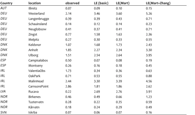
mean stdev mean stdev RMSE correlation
total PM10 25.58 10.63 13.81 9.68 15.39 0.68 NO3 3.20 3.02 3.70 3.12 2.48 0.70 NH4 1.59 1.29 1.90 1.33 1.05 0.71 SO4 1.98 1.63 2.20 1.39 1.43 0.59 sea salt 1.42 1.19 2.81 2.84 0.54 black carbon 0.46 0.43 0.89 0.44 0.75 prim PM10 0.91 0.55 prim PM2.5 2.39 1.23
Statistical comparison between modelled and observed concentrations of PM10 and their components. We
compared modelled and observed mean concentrations and standard deviations (stdev) and provided root mean square errors (RMSE) and correlation coefficients. All statistical parameters were determined based on daily data for the individual stations and were then averaged. Sea salt observations were not well constrained and only the correlation coefficient is given. The same applies to black carbon, for which the observations were estimated from black smoke observations (see text).
and modelled values were given separately for each model. LOTOS-EUROS still missed a considerable amount of ances, but the percentage of the correctly predicted exceed-ances was 60 %. Inspection of the time series and the scatter plots for PM10, indicated that the periods with exceedances were generally captured in modelled high concentrations (but not above 50 μg/m3). This may be explained by the nature of a model to represent average conditions (through average emissions, parameterisations, etc). A number of exceedances was caused by sources not included in the model, such as fire works at New Year’s Eve and Easter Fires. The performance of the model as a function of measured PM10 may indicate which components add to the underestimation as a function of PM mass, and is discussed in the next section.
The fact that the LOTOS-EUROS model performs better compared to the persistence model, may indicate that it is worthwhile to investigate if the model would be suitable for
actual forecasting purposes. The model which is used now, PROPART, is only slightly better than the persistence model (Manders et al., 2008). In contrast to a statistical model such as PROPART, LOTOS-EUROS provides more detailed knowl-edge on PM composition and origin as well as maps and time evolution, which enhances the possibility of communicating the results to the general public (Manders et al., 2008).
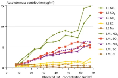
Variability of composition 3.3.3
Here we will address if the model components show similar behaviour as a function of PM10 to the observed behaviour. Figure 3.6 shows the contribution of several components to PM10 as a function of the PM10 concentration. LOTOS-EUROS results showed a more or less linear relationship between PM10 and NO3, SO4 and NH4. Observations yielded similar results. Ammonium and sulfate equally contributed to the PM mass in both the model and the observations. In the obser-vations nitrate contributed the most with a slight increase
Comparison between modelled and measured PM10 concentrations for all LML locations. The comparison was made for every season: winter (DJF), spring (MAM), summer (JJA) and autumn (SON). The data represent all model– measurement pairs during each season for 15 LML stations. The fit parameters are given above each panel.
Figure 3.4 0 10 20 30 40 50 60 Modeled PM10 (µg/m3) 0 20 40 60 80 100 120 Measured PM DJF MAM JJA SON 10 (µg/m3) y=8.31073 + 1.5366x R2=0.52225 0 10 20 30 40 50 60 Modeled PM10 (µg/m3) 0 20 40 60 80 100 120 Measured PM10 (µg/m 3) y=7.4701 + 1.4224x R2=0.46631 0 10 20 30 40 50 60 Modeled PM10 (µg/m3) 0 20 40 60 80 100 120 Measured PM10 (µg/m 3) y=13.533 + 0.75963x R2=0.25569 0 10 20 30 40 50 60 Modeled PM10 (µg/m3) 0 20 40 60 80 100 120 Measured PM10 (µg/m 3) y=9.057 + 1.3102x R2=0.51309
Base case 23
towards high PM concentrations. This pattern was followed by the model, although the model slightly underestimated nitrate at high concentrations. In both the model and the observations, the elemental carbon concentrations tended to be relatively higher at low concentrations ranges.
As a sea salt tracer, sodium (Na) was modelled and chloride (Cl) was observed. In Figure 3.6, neither the observed nor the modelled tracer was transformed to a sea salt equivalent. Note that the chloride-based concentrations were not reliable because of the abovementioned reasons. Nevertheless, the relative contribution to total PM10 could be deduced from the results. For sea salt, the contribution did not increase with increasing total PM10 but rather decreased. The highest con-centrations were found for relatively low total PM10 concen-trations. This behaviour was found in the observations as well as in the model, and could be easily explained by the high sea salt loads in periods with fast transport from the sea, which
represents the clean sector in the Netherlands. These results indicate that sea salt did not contribute a large mass fraction on the days with high PM concentrations (exceedance days).
The analysis revealed that the model captured the vari-ability of the substances that could be evaluated. There is no indication that these components could explain the gap between observed and modelled concentrations. In addition, there was no large mismatch between the observed and modelled contributions of these components over the full range of observed PM10 levels. This means that the missing mass is associated with the non-modelled components and those components that could not be evaluated through measurements.
Observed and modelled average PM10 concentrations for Vredepeel (LML131), 2005. Both the LOTOS-EUROS model (red) and the bias-corrected model (blue) are shown.
Figure 3.5
Jan Mar May Jul Sep Nov
0 10 20 30 40 50 60 70 PM10 concentration (µg/m 3) Measured LOTOS-EUROS Bias corrected Vredepeel, 2005
Observed and modelled average PM10 concentration
Feb Apr Jun Aug Oct Dec
Average statistical properties of the model for comparing measurements of PM10
parameter le_bc le persistence
mean 26.45 13.25 26.51 bias -0.03 -13.23 0.02 residue 6.49 13.40 7.64 rmse 9.06 16.34 10.99 stde 9.06 9.60 10.99 skvar 0.70 0.50 1.00 correlation 0.70 0.68 0.63 hit rate 49.21 8.30 46.32 predicted 50-200 380 1.00 991 observed 50-200 1003 1003 983 %correct 50-200 61.32 100.00 42.48 datacoverage 0.96 0.96 0.94
Average statistical properties of the model for comparing measurements of PM10 between 2004 and 2006. All
parameters were calculated for each station for the three years of daily data and subsequently averaged to provide one value for each parameter.
Discussion and conclusions
3.4
In this chapter, we have presented the annual mean distribu-tion of PM10 and its components, as calculated by the model. Furthermore, we have examined the performance of the LOTOS-EUROS model by comparing it to observations in the Netherlands. LOTOS-EUROS was capable of modelling the temporal behaviour of PM10 concentrations rather well. However, the absolute concentration was not captured and a systematic bias existed between the modelled and the measured concentrations. On average, the underestimation by LOTOS-EUROS was 11.7 µg/m3. Verification of the second-ary inorganic components, sea salt and EC indicated a good temporal behaviour and did not indicate that one of these components contributed largely to this bias. In addition, analysis of the model performance as a function of PM10 revealed that the model captured the variability of the sub-stances that could be evaluated. This means that the missing
mass is indeed associated with the non-modelled components and those components that could not be evaluated through measurements.
Similar to other models for Europe, LOTOS-EUROS has a considerable bias for PM10. On average, the underestimation by LOTOS-EUROS was 11.7 µg/m3. Compared to the underes-timation obtained by OPS (12 μg/m3) one could conclude that the underestimation in both models was very similar. This is no surprise, as both LOTOS-EUROS and OPS include the same components. PM10 is modelled as:
PM10 = SO4 + NO3 + NH4 + PPM10 + sea salt
In reality, PM10 consists of more substances:
PM10 = SO4 + NO3 + NH4 + EC + POM + SOA + PPMunknown + sea salt + CM + water.
Modelled and observed absolute (top) and relative (bottom) contribution of NO3, SO4, NH4, EC and sea salt in Vredepeel versus observed total PM10. Note that the observed (Cl) and modelled (Na) sea salt tracers were not transformed to a sea salt equivalent and were meant to illustrate their behaviour. Observed EC concentrations were derived from black smoke measurements.
Figure 3.6 0 10 20 30 40 50 60 70 Observed PM10 concentration (µg/m3) 0 5 10
15 Absolute mass contribution (µg/m
3 ) LE SO4 LE NH4 LE NO3 LE Na LE EC LML SO4 LML NO3 LML NH4 LML Cl LML EC
NO3, SO4, NH4, EC and sea salt in Vredepeel versus observed total PM10
Modelled and observed absolute and relative contribution
0 10 20 30 40 50 60 70 Observed PM10 concentration (µg/m3) 0.00 0.05 0.10 0.15 0.20
0.25 Relative mass contribution (µg/m
3) LE SO4 LE NH4 LE NO3 LE Na LE EC LML SO4 LML NO3 LML NH4 LML Cl LML EC
Base case 25
Crustal matter (CM) and secondary organic aerosols (SOAs) had not yet been incorporated in the model version prior the start of the BOP project, because of a lack of solid knowledge on emission strengths for CM and formation routes for SOA. Crustal matter may have contributed 3-5 µg/m3 for the Nether-lands (see Chapter 5) and could explain a large fraction of the bias. In addition, but much more uncertain, SOA also could have added a significant mass. First steps were taken in Chap-ters 5 and 6 to include these components and pursue mass closure. Finally, it was posed that PM10 measurements include a portion of water, which might contribute to the systematic underestimation of the observed levels (Tsyro, 2005).
The emission data that were used here did not provide chemically speciated data, which made it hard to verify the primary components. Primary material should be distin-guished in elemental carbon and primary organic matter. Furthermore, a part of the primary PM remains unidentified. This small fraction derives mainly from mechanical wear and may contain a considerable amount of metal. The distinction will be made during the BOP programme by using a chemi-cally specified emission database for elemental carbon (EC) and primary organic matter (POM). Having data on organic matter would allow comparing model results with OC and TC measurements.
We also showed that no firm conclusions could be drawn on the model performance for sea salt. The comparison shown above was hampered by the limited usability of the chloride measurements from the LML LVS samplers. The measure-ments have a rather undefined cut-size and were therefore difficult to compare to the model results. In addition, chloride is replaced by sulphate and nitrate through reaction of sulphuric and nitric acid with sea salt in ambient air. Hence, without correction, the sea salt estimates based on chloride represented the lower limit. Finally, the measurements were often below the detection limit which posed a problem with the data handling and appreciation. Hence, the model results for sea salt were not extensively validated for Dutch condi-tions. The same applies to European conditions, because of a lack of observation data. In Chapter 4, we updated the model description to a combination of two emission parameterisa-tions that would be considered to be state-of-the-art. The BOP measurements together with an effort of compiling foreign data, provide the first opportunity for a more exten-sive validation than presented above.
A CTM such as the LOTOS-EUROS model, is an approxima-tion of reality and therefore describes average condiapproxima-tions (through emissions, parameterisations, etc). Observations, however, are often influenced by contributions derived from events, such as Easter Fires or fire works. Also, long-range transport of forest-fire plumes or dust storms may occasion-ally reach the Netherlands (Hodzic et al., 2006; Birmili et al., 2007). These events may be included in models using routines for wind blown dust (e.g. Bessagnet et al., 2008) or satellite derived fire counts in combination with an emission module. The magnitude of the emissions and the specific conditions during such events are difficult to capture adequately. Data assimilation of both in-situ and remote sensing observations (in and upwind from the Netherlands) may therefore aid the
air quality analysis. LOTOS-EUROS is equipped with a data assimilation system (e.g. Van Loon et al., 2001; Barbu et al., 2008; Denby et al., 2008). The challenges regarding data assimilation are many but its use for air quality assessment should be investigated.
We identified three substances for which the uncertainties in the modelling needed to be reduced. These were sea salt, crustal material and organic carbon. The next three chap-ters describe efforts of improving the modelling of these components.