Evaluation of Automated Registration techniques for BIM Geometry and Corresponding Point Clouds

THESIS

Evaluation of Automated Registration techniques for BIM Geometry

and Corresponding Point Clouds

Word count: 29,871

Chia Honoré

Student number: 01508799

Eva Landuyt

Student number: 01708410

Supervisor: Prof. Dr. Ing. Greet Deruyter,

Counsellor: Noaman Akbar Sheik

Master’s dissertation submitted in order to obtain the academic degree of Master of Science in de industriële wetenschappen: landmeten

THESIS

Evaluation of Automated Registration techniques for BIM Geometry and

Corresponding Point Clouds

Word count: 29,871

Chia Honoré

Student number: 01508799

Eva Landuyt

Student number: 01708410

Supervisor: Prof. Dr. Ing. Greet Deruyter,

Counsellor: Noaman Akbar Sheik

Master’s dissertation submitted in order to obtain the academic degree of Master of Science in de industriële wetenschappen: landmeten

Foreword

This thesis is the final part of our master’s degree: Master of Science in Land Survey Engineering Technology. During the education, we both became interested in the use of BIM in construction and wondered how it can chance the construction sector. Thus, we started this research to learn more about BIM implementations and automation in construction.

In addition, we want to take a moment to reflect on the process involved in this graduation project. It was a difficult but informative project due to the fact that there is a huge interest in this topic, which resulted in a lot of innovations these recent years.

We would like to thank our mentors prof. dr. Ing. Deruyter and Phd student Noaman Akbar Sheik for their time, assistance and kindness toward us. Their constructive feedback always gave us more motivation to continue.

Further we would like to thank the hospitality of Timothy Nuttens, BIM manager at “Agentschap Wegen en Verkeer”, who invited us at his office and gave us information as in scientific articles and researches. He even gave a short presentation about BIM at the campus Sterre in Ghent, to which we were invited. Lastly, we would both like to express our thanks separately. Chia wants to thank the church to stay open and provide study space in summer vacation. Eva has special thanks to her family for staying calm and supportive. Also, we thank each other for not giving up and for staying focused and committed. We want to wish you all a pleasant time reading this thesis, and we hope you will get inspired in BIM and in the automated registration techniques.

Abstract

Nowadays, building information modelling (BIM) is widely used in the construction industry to enhance project performance from design to construction. Construction projects are characterised as a dynamic process, in which the planning continuously deviates from the actual situation. Therefore, 3D point cloud data is used to capture the accurate conditions of the construction, but the processing of today’s large point clouds is time-consuming and time is money for all construction projects. Fortunate, new techniques are being developed to automate the progress monitoring process. When point cloud data are adopted for construction applications, a series of data processing procedures are required to obtain the desired output. A processing step is the registration of different point clouds. The aim of this registration step is a coarse alignment, which can then be improved by a fine registration. Although research on ACCPM is in full development and different automated registration techniques already exist, a performance evaluation of these algorithms is not available. The research presented in this thesis focuses on evaluating these registration techniques based on speed and accuracy. In summary, the results of the experiments for coarse registration indicate that RANSAC has a much higher processing time than the Fast Global registration. In general for fine registration, ICP point-to-plane performed faster and needed less maximum iterations to converge through all tests. The results of the experiments suggest that ICP works well in most cases given enough overlap between the point clouds. The research would have been more interesting if more algorithms could have been included and compared to obtain further in-depth information.

Keywords: BIM, data-acquisition, construction planning, 3D registration algorithms, monitoring process, point clouds, performance evaluation

In de bouwsector wordt tegenwoordig veel gebruik gemaakt van Building Information Modelling om de projectprestaties vanaf het ontwerp tot de constructie oplevering te verbeteren. Bouwprojecten kenmerken zich als een dynamisch proces, waarbij de planning continu afwijkt van de werkelijke situatie. Echter door de ontwerpwijzigingen in de constructiefase weerspiegelt de geplande BIM vaak niet de as-built omstandigheden van het project. Daarom worden 3D puntenwolken gebruikt om de constructie nauwkeurig vast te leggen, maar de verwerking van de hedendaagse, grote puntenwolken is tijdrovend en resulteert in hogere kosten voor bouwprojecten. Gelukkig worden nieuwe technieken ontwikkeld om de vooruitgang te automatiseren. Wanneer puntenwolken gebruikt worden voor bouwtoepassingen, zijn een reeks verwerkingsprocedures vereist om de gewenste output te verkrijgen. Een van die verwerkingsstappen is de registratie van verschillende puntenwolken en het doel van deze registratiestap is het bekomen van een grove registratie die vervolgens kan verbeterd worden door een fijne registratie. Het onderzoek in deze thesis is gericht op het evalueren van de snelheid en nauwkeurigheid van deze registratietechnieken. Samenvattend geven de resultaten van de experimenten voor grove registratie aan dat RANSAC een veel langere verwerkingstijd heeft dan de Fast Global

registratie. In het algemeen presteerde ICP point-to-plane voor fijne registratie sneller en had het minder maximale iteraties nodig om te convergeren voor alle tests. De resultaten van de experimenten suggereren dat ICP in de meeste gevallen goed werkt bij voldoende overlap tussen de puntenwolken. Het onderzoek zou interessanter zijn geweest als er meer algoritmen hadden kunnen worden opgenomen en vergeleken om meer diepgaande informatie te verkrijgen.

Kernwoorden: BIM, data-acquisitie, constructie planning, 3D registratie algoritmes , automatisering, monitoring proces, puntenwolken, prestatie-evaluatie

1

Evaluation of Automated Registration techniques for

BIM Geometry and Corresponding Point Clouds

Word count: 9934 Chia Honoré, Eva Landuyt Supervisor: Prof. Dr. Ing. G. Deruyter

Abstract: Nowadays, building information modelling (BIM) is widely used in the construction industry to enhance project performance from design to construction. Construction projects are characterized as a dynamic process, in which the planning continuously deviates from the actual situation. Therefore, 3D point cloud data is used to capture the accurate conditions of the construction, but the processing of today’s large point clouds is time-consuming and time is money for all construction projects. Fortunate, new techniques are being developed to automate the progress monitoring process. When point cloud data are adopted for construction applications, a series of data processing procedures are required to obtain the desired output. A processing step is the registration of different point clouds. The aim of this registration step is a coarse alignment, which can then be improved by a fine registration. Although research on ACCPM is in full development and different automated registration techniques already exist, a performance evaluation of these algorithms is not available. The research presented in this thesis focuses on evaluating these registration techniques based on speed and accuracy . In summary, the results of the experiments for coarse registration indicate that RANSAC has a much higher processing time than the Fast Global registration. In general for fine registration, ICP point-to-plane performed faster and needed less maximum iterations to converge through all tests. The results of the experiments suggest that ICP works well in most cases given enough overlap between the point clouds. The research would have been more interesting if more algorithms could have been included and compared to obtain further in-depth information.

Keywords: BIM, data-acquisition, construction planning, 3D registration algorithms, monitoring process, point clouds, performance evaluation

I. INTRODUCTION

Most construction projects consist of numerous labour, materials, equipment and processes and may become too large and complex to monitor manually [1, 2]. Therefore, the construction industry wants to automate the monitoring process, which requires the development of new methodologies that allow automatic recognition of as-built performance and visualisation of construction progress [3].

With the development of point cloud data acquisition methods and processing capabilities, point cloud data has received more and more attention and has been recommended as the most suitable data source for progress monitoring [4]. Since each application area has its own requirements, many algorithms have been proposed [5].

Automated point cloud registration focuses on the coarse-to-fine registration strategy [6], which starts with an initial rough alignment followed by a fine registration to obtain an optimal

alignment and to get the most precise transformation [7-11]. Therefore, the rigid registration methods are classified into coarse and fine registration algorithms [6]. The goal of this research is to evaluate some well-known registration algorithms used for aligning an built point cloud with the as-planned point cloud generated from a Building Information Model (BIM) and to establish an registration algorithm performance evaluation based on two criteria: accuracy and speed.

II. LITERATURE

A. Automated progress monitoring

Monitoring the current state and progress of a project is a crucial task of construction project management and requires regularly accurate progress information [12]. Detecting deviations in an early stage between the as-built and as-planned progress enables decisionmakers to take action and can prevent potential upcoming delays, costs and even sometimes environmental impacts [3, 13, 14]. Nevertheless, traditional progress monitoring based on visual observations and traditional surveying methods is labour-intensive due to their dynamic and complex nature [2]. Therefore, a BIM can help to automate the progress monitoring [13, 14]. Using a BIM during the design and construction phase of a project’s life cycle, may reduce rework, improve efficiency and minimize unexpected costs [15, 16].

A BIM may be defined as a comprehensive three-dimensional (3D) digital representation of a facility and a rich source of information in terms of 3D geometry and semantic information about the building component types, such as the used material and spatial relationships [12, 13]. An ideal BIM concept in which all semantic data is connected with a process schedule, which consist of all construction tasks and its duration, is called a 4D BIM. This way, it combines all relevant information needed to complete the construction process, and enables monitoring and optimization of construction processes [3, 17, 18]. Additionally, a 5D BIM can be created by linking the costs to the components of a 4D BIM and can further be used for risk analyses or financing [19].

A procedure referred to as Automated Continuous Construction Progress Monitoring (ACCPM) documents and accommodates all changes in construction and consists of following steps after receiving the merged point cloud: data preparation, scene-to-model registration, object recognition and schedule update [20]. The main focus in ACCPM is the

2 comparison of the as-built and the as-planned state. Design

models may not accurately represent the as-built state, so to define these deviations, detailed information about the current progress is necessary [21]. When a reliable as-planned 4D BIM exists the Scan-vs-BIM method can be used for progress monitoring, which is the process of comparing an as-built with the planned 4D model [14, 21-23]. Another option for progress monitoring, when no planned BIM is available, is generating a BIM from the as-built model using the Scan-to-BIM method, which is known as the process of transferring point clouds into BIM’s [13, 15, 18, 24]. Eventually, the last step of ACCPM is the identification and visualisation of construction tasks that are behind schedule with the purpose to automatically update the tasks status and schedule [15, 25].

Planning plays an important role in the optimisation and management of a construction project [26]. The key elements in construction planning are activities, durations, sequences, and relationships between the tasks. Early assessment of the as-built status during construction is required for effective and efficient tasks planning [27]. Therefore, it is necessary to capture data regularly by periodic monitoring to update the project’s schedule of an entire construction site. Then, the actual schedule can be compared with the planned schedule to identify activities behind schedule by comparing point cloud data, acquired over time, with the corresponding as-designed 4D BIM [27, 28]. The comparison requires accurate 3D registration and should be performed with care (Sehgal et al. 2010).

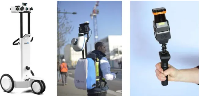
B. Data acquisition

Point cloud data is the most suitable data source for ACCPM as it captures the geometries of construction sites [13]. To automate the construction progress monitoring, several acquisition methods such as laser scanning, photogrammetry and videogrammetry can be used to generate a point cloud of the current progress [14, 29]. Choosing a specific acquisition method determines some properties of the point cloud. They all have their pros and cons but all provide a more or less accurate reconstruction of a surface [29].

1) Laser scanning

For ACCPM, only terrestrial laser scanners (TLS) are used. They use a ground-based method that rapidly acquires accurate, dense 3D point clouds of object surfaces by laser technology [30]. Laser scanning is based on Light Detection and Ranging (LiDAR) technology, which calculates the distance between the scanner and the object through emission and detection of laser beams [31]. Based on their working principle, laser scanners are divided into three categories: pulse based (Time-of-Flight), phase based and Wave Form Digitizer (WFD) scanners [2]. Based on movement, TLS can be classified into static laser scanners and mobile laser scanners (MLS) [2]. The performance of a laser scanner is determined by important factors, such as the angular resolution, the scanning speed and the range requirement [24].

Generally, laser scanners have a large measurement range, high level of detail, higher acquisition speed in comparison with traditional survey instruments such as total station and are independent on ambient light [6, 10, 15, 21, 27, 31]. The chosen level of detail has an influence on the processing time [10].Other disadvantages of laser scanning are the higher equipment cost, slow warm-up time, the need for a clear line of sight, the difficulty of using it in congested interior work as they are not easily portable, the need for engaging experts for

equipment handling and a regular sensor calibration [13, 27]. They are also easily affected by external light sources, reflectivity, colour and roughness of the object [31]. Error sources may affect the accuracy of laser scanning measurements, and can be classified into four categories: instrumental, object-related, environmental and methodological errors [31]. The key for qualitative data is to optimize scanning parameters, such as the resolution and avoid collecting redundant scan data [28]. During both the scanning process and the processing are MLS faster than static laser scanners [2, 32]. On the other hand, the resulting point clouds have a lower general quality compared to static laser scanners, so the current MM systems compromises on the general quality of the point clouds [32]. It is important to establish a relationship so that the acquired data fulfil the required quality [31].

Since most construction sites are large, the data acquisition for static laser scanners involves capturing 3D data from different views [33]. The accuracy of the resulted point cloud is mainly determined by the data registration method which combines multiple point clouds in the same reference system [2, 33-35]. Point clouds can be merges by pairwise or multiview registration methods. A pairwise registration calculates a rigid transformation between two subsequent point clouds, while the multiview registration process takes multiple point clouds into account. Multiview registration is significantly more difficult, due to three challenges: attempting to recover the view orders, estimating pairwise rigid transformations, and determining absolute poses (orientations) [30]. Georeferencing the data can make sure that the acquired point cloud and the BIM have a rough alignment in the same coordinate system, which facilitates the automation process that uses the coarse-to-fine strategy [6]. Georeferencing means aligning the scans and also transferring the dataset to an absolute coordinate system. [31]. This can be done direct if the static laser scanner is positioned over control points or by GNSS. Indirect georeferencing is possible by determining the coordinates of targets or points of interest using a total station or GNSS [31].

2) Video/photogrammetry

Over the years, photogrammetry has gained al lot of popularity due to the wide availability, the affordable price and ease of use of the required equipment and the maturity of photogrammetric software packages, such as Autodesk Recap, Agisoft Metashape, etc. It’s an economical and effective technique at large scale and has been widely used in construction to obtain a 3D point cloud required for as-built documentation, 3D modelling, localisation and map production [2, 12, 24, 27].

Videogrammetry differs from photogrammetry as it takes video streams as an input instead of a collection of images. [2, 8]. A little human intervention in the reconstruction process results in a quicker and an improved accuracy since the search of target points in different images can be achieved by measuring or tracking interesting features based on the previous frame(s) [2, 24]. However, it may also have issues and challenges such as the higher volume of data as well as more noise in the final point cloud than still images. This is due to a reduction in image quality [14].

C. Data preparation

Data processing procedures are required to obtain the desired outputs from the point clouds. It refers to the process of

3 transforming the raw point clouds into a final deliverable [2].

Although the measurement system has a significant importance on the quality of the desired output, the different preparation steps are explained for the process after receiving the merged point clouds, regardless of which acquisition method is used [36].

Generally, before processing the point clouds errors due to extreme environmental conditions or to human mistakes are removed from the data set before the merged point cloud is created [31]. Whereas, noise may effect the precision of the scene-to-model registration, a sequence of filters can be applied to each of the clouds being registered to remove redundant and erroneous data to improve the registration [31, 37]. However, removing noise has to be done with caution, because e.g. features can be lost when over-smoothing the data set or removing too many points [2, 31, 38].

Another data preparation step is subsampling a point cloud, which can be performed to obtain a common resolution for two data sets [39]. Using this technique, a proper reduction of the original point cloud size can be achieved without losing valuable features [31]. Therefore, resampling can be used to improve a point-to-point registration [40].

B. Coarse registration algorithms

If he point clouds are pre-aligned, georeferenced, or have known correspondences, the coarse registration step is unnecessary [6, 33]. Otherwise, the coarse-to-fine strategy is used to roughly align two point clouds to prepare them for fine registration [6, 39]. Therefore, coarse registration methods are generally less accurate and more robust than fine registration methods [2]. A few known algorithms are discussed.

1) RANSAC

The RAndom SAmple Consensus (RANSAC) algorithm was introduced by Fischler and Bolles with the purpose of fitting a model to experimental data for solving the Location Determination Problem [41]. In Figure 1, a specific example of RANSAC is given in which RANSAC tries to fit a line into the model. A good fit will be found by sampling a sufficient number of subsets and by using the subset that contains the most inliers [42]. In this example, the best current fit is illustrated bottom left side with 19 inliers.

Figure 1: Example of RANSAC fitting a line [43]

The iterative algorithm starts by randomly selecting three different points from the source point cloud and three from the target point cloud to form a pair of bases in correspondence. To estimate candidate transformations, translation and rotation parameters, the base pairs are registered. Then, those points in

the source point cloud whose Euclidean distances to their corresponding points in the target point cloud are smaller than a predefined inlier threshold are counted [44, 45]. The process continues by randomly selecting other combination of three point pairs to derive different candidate transformations that may improve the current best fit. The algorithm repeats the voting process enough times to ensure with high probability that it finds a good solution with enough correspondences or until it has reached the number of allowed iterations [46].

The RANSAC-based algorithm is a well-known algorithm for coarse registration of point clouds due to the good results. However, a major drawback is the high computational cost, especially when handling data sets with a lot of noise [6, 47]. Although random sample based algorithms are somehow robust to noise, outliers and repetitive structures, the total number or trials increases exponentially with a high outlier ratio [45, 47]. In general, RANSAC-based algorithms may not give a satisfactory result, because RANSAC is a randomized heuristic [42]. Therefore, several improvements of RANSAC are developed such as: MSAC, MLESAC, 3D MLESAC, LO-RANSAC,RANSAM and PROSAC.

2) 4PCS

In 2008 Aiger, Mitra and Cohen-Or introduced the RANSAC-based 4-points congruent sets (4PCS) algorithm. This method is based on geometric consistency by using four point pairs and it uses wide bases instead of local ones. The advantage of using a wide base is creating a robust algorithm as a wide base is in general more stable. Moreover, using 4-point bases surprisingly result in a significantly reduced number of trials. The combination of a wide base and the largest common point set makes the algorithm resilient to noise and outliers. Therefore, prefiltering and denoising the point cloud is not necessary [46].

The first step in the algorithm is selecting four coplanar points in the source set, which starts with randomly selecting three points. The fourth point is chosen such that the four points together form a wide base which is approximate coplanar. Secondly, the algorithms searches all subsets of 4-points from the given point cloud that are approximately congruent to the source point cloud by calculating the corresponding distance. The chosen set of coplanar points X={a, b, c, d} in the source point cloud, not all collinear, defines two independent ratios of three collinear points. In Figure 31 lines ab and cd intersect at an intermediate point e and they define ratio’s 𝑟1 and 𝑟2, which

are invariant under affine transformation [46]. The algorithms calculates distances ||ab|| and ||cd|| in the source point cloud. Then, by using the ratios r1 and r2, the intermediate points e1

and e2 are calculated, respectively with equation (1) and (2), for

each pair of points 𝑞1 and 𝑞2 in the given point cloud.

𝑒1= 𝑞1+ 𝑟1 (𝑞2− 𝑞1) (1)

𝑒2= 𝑞1+ 𝑟2(𝑞2− 𝑞1) (2)

The only points considered in the given point cloud, are those point pairs at the same distance as the distances calculated in the source point cloud. If two calculated intermediate points coincide (e1  e2), the two pair of points probably correspond

to a 4-points set that is an affine transformed copy. Due to noise, these intermediate points end up being nearby points and therefore the algorithms searches for all points associated with 𝑟1 that are in the neighbourhood of points associated with 𝑟2

4 Figure 2: Extracting affine invariant congruent 4-points [46]

The next step is computing the corresponding transformations for different bases of point pairs. Finally, the best transformation matrix is chosen and the two 4-points sets can be aligned, up to some allowed tolerance , using rigid transformation [46].

The algorithm can be improved, because the 4PCS-based method has two main weaknesses. It is still a time consuming procedure for large point clouds, since it has a quadratic time complexity and it assumes that congruent sets are invariant to the rigid transformation [30]. Therefore, some more efficient variants of 4PCS have been proposed, where the main improvements include reducing the number of candidate points, enhancing the robustness, implementing large-scale scenes and decreasing the failure rate Some examples of improved variants are: S4PCS, G-4PCS, SG-4PCS, K-4PCS, SK-4PCS, V4PCS, A4PCS and 4 Planes (instead of Points) Congruent Sets [30, 45].

3) The fast global registration

Another RANSAC-based algorithm is the Fast global registration (2016) . It uses initial correspondences which are selected using the FPFH feature. Similar to RANSAC, an error function is optimized such that the distances between corresponding points are minimized. The big difference is that the correspondences are not recomputed during the optimization to achieve high computational efficiency. For this reason, the algorithm is supposed to be faster than RANSAC [48].

4) PCA

In 1998, Chung et al. presented a registration algorithm based on PCA that uses the covariance matrix to determine the transformation between two point clouds [49]. If the covariance matrix of two point clouds differs from the identity matrix, a rough registration can be obtained by simply aligning the eigenvectors of their covariance matrices [11]. According to the eigenvalues, these vectors are mapped into three axes [20, 50]. Figure 3 illustrates these vectors, which represent the principal axes of the data and in which the length of the vector is an indication of how important that axis is in describing the distribution of the data. The projection of each data point onto the principal axis are the “principal components” of the data [51].

Figure 4 shows the projected points (darker points) onto the principal axis and it reveals that PCA reduces the dimensions of the original data (lighter colour). The information along the least important principal axis or axes is removed, while leaving only the components of the data with the highest variance [51]. In point cloud registration, this method is used to find and identify the principal axes that describe the shape of a point and

are used for the estimation of the relative position and orientation [10]. The basic idea of PCA is to seek a projection that best represents the data [52]. PCA gained popularity in different fields and should work well [10, 50]. It is mainly advantageous, because it is simple, fast, and applicable to most of 3D models. Nevertheless, one outlier can have an arbitrarily large effect on the result due to the lack of robustness in the least squares method. Moreover, the principal axes derived by PCA might be quite different for some similar shapes due to some small local difference between shapes [50].

Figure 3: Describing the distribution of data using the principal axes of PCA [51]

Figure 4: Original data projected onto a principal axis [51]

C. Fine registration algorithms

The most common registration algorithm for fine registration is ICP due to its simplicity and high usability [33, 45, 53, 54]. The goal is to refine the transformation matrix by minimizing a predefined error function [9]. Although ICP is extremely dependent on a good initialization and good overlap between point clouds, the algorithm converges relatively quickly [10, 11, 30, 55, 56]. In addition, an inaccurate initial alignment or a low overlap between point clouds may deteriorate the accuracy of registration severely and besides a good coarse registration reduces the number of iterations [10, 11, 30, 56-58]. In general, ICP algorithms have a high accuracy and stability but low efficiency in terms of speed when registering large-scale, high-density point cloud scenes [6, 9, 54, 58, 59].

The algorithm refines the transformation matrix by iteratively minimizing the distances between tentative correspondences, known as closest points, until convergence [45, 54]. The different steps of the ICP scheme are given in Figure 5.

5 Figure 5: ICP overview scheme [11]

In the first step, given an initial coarse registration, the ICP algorithm is looking for pairs of closest points between two different point clouds. A number of points are selected in the target point cloud and then, based on a nearest neighbour approach, the corresponding points are searched and identified in the source point cloud [6, 58]. Next, translation and rotation parameters are calculated through SVD in order to obtain an initial estimate of the affine transformation matrix that aligns both point clouds [9, 11]. Then the transformation is estimated from the closest points by minimizing the error function [45]. Consider a set of source points Q, being registered to a set of source points P by using a rotation matrix R and a translation vector t [60]. The error function is chosen as [60]:

𝐸(𝑅, 𝑡) = ∑𝑁𝑖=1‖𝑅𝑝𝑖+ 𝑡 − 𝑞𝑖‖² (4)

where 𝑞𝑖,𝑛 is the closest point in data set Q to the point 𝑝𝑖,𝑛

in data set P, and n is the current iteration number. The values Rn and tn that minimize this function (for each iteration) are

performed iterative by transforming the source points by the calculated Rn and Tn until the registration converges

The initialization step also consists of choosing a stopping criterion, such as the Euclidian distance between closest points, because the search radius effects the calculation time, depends on the cloud point density and the initial position estimate. The calculation of the Euclidian distance, which is based on a least squares method is presented as followed [9, 36, 59]:

𝑑 = 𝑚𝑖𝑛‖𝑝𝑖− 𝑞𝑗‖ (5)

where pi is the closest point of interest, qi the corresponding

point of the source point set, i ∈ 0,1,...,N, and N is the number of points in target point cloud [59]. Note that the pair (qi, pj) is

initially a tentative correspondence, which become a true correspondence when convergence to a global minimum is attained [58].

Figure 6 illustrates how the error function f(R,T) of the ICP registration algorithm is minimized iteratively. As long as the error decreases and mean square error is greater than a certain threshold, ICP algorithm will determine corresponding points, compute rotation R and translation t through SVD to transform the target point cloud and recalculate the error function [11].

Figure 6: ICP least square approach [53]

The geometric registration problems have led to multiple variations such as LM-ICP, Generalized ICP, Global optimal ICP and ICP with invariant Features, who seek to improve robustness, speed and accuracy [7, 56, 58, 59]. The ICP algorithm needs to find corresponding points in each iteration, which is time consuming. Therefore, techniques for improving speed are subsampling, closest point computational and distance formulation.

The most important factor affecting the speed of ICP is the point-to-point or point-to-plane distance (Castellan & Bartoli, 2012). These two approaches only differ in their definition of point correspondences, shown in Figure 7 and Figure 8 (Bellekens et al., 2015).

Figure 7: Distance formulation. Left: to-point; Right: Point-to-plane; (Kjer & Wilm, 2010)

Figure 8: Distance formulation (2D). Left: Point-to-point; Right: Point-to-plane; (Yue, 2019)

Overall, a transformation of the reading cloud is determined by minimizing an objective function. This is either the sum of squared distances between the corresponding points (point-to-point) or between a point from the reading cloud and the tangent plane of the corresponding point from the reference cloud (point-to-plane) (Castellan & Bartoli, 2012). The ICP point-to-plane algorithm assumes that the local neighbourhood of a point in a point cloud is coplanar. Instead of directly minimizing the Euclidean distance between corresponding points, the scalar projection of this distance can then be minimized onto the planar surface defined by the normal vector n (Bellekens et al., 2015; Kjer & Wilm, 2010). A point-to-plane approach leads to faster convergence and more accurate ICP than a point-to-point distance formulation (Al-Nuaimi, 2017; Gu et al., 2020; Xian et al., 2016).

On the other hand, the accuracy of the registration can be improved by an outlier rejection strategy and additional information such as colour and texture or local geometric properties [58, 61]. Furthermore, in order to improve the robustness of the registration, the correspondences can be weighted [58].

D. Evaluation

The choice of an algorithm generally depends on important characteristics, such as accuracy, computational complexity, and convergence rate and therefore it depends on the application of interest. Evaluation parameters for accuracy are ground-truth (GT), root mean square distance/error (RMSD/RMSE), distance/translation error and rotation error [6]. Another evaluation criteria is the efficiency, also called the computational cost. It can be measured by the execution time in milliseconds which can be displayed on the screen [4, 9, 29, 36]. Furthermore, the robustness can be tested for different challenges such as input data, noise, sampling, overlap area and acquisition [10]. By performing error analysis on the registration results, it is possible to select the most suitable registration method [6].

6 III. EXPERIMENTS

A. Test data

An important aspect in testing and comparing the registration algorithms are the test data. Since little house, St. Marys and the sports hall, shown in Table 1, are not perfect due to data acquisition and environmental factors, perfect clean BIM’s were created using the ArchiCAD software. Each model has his own recognizable in shape (Table 2) to test the influence of the geometry. Each building has his own difficulties. Little house has an imperfect geometry, St. Marys does not include the outside and the as-built of sports hall contains much noise and is acquired through photogrammetry whereas the as-planned is clean and acquired through laser scanning.

Table 1: Realistic models

As-planned As-built Little house St. Marys Sport s hall

Table 2: Geometry - theoretical models

Cube house Box house Tall house L house

B. Evaluation criteria

The aim of this research is to compare some well-known automated registration techniques by using different point clouds for the purpose of construction. Although there are many registration algorithms developed, in this research only four open source algorithms were compared: ICP point-to-point, ICP point-to-plane, RANSAC and Fast Global registration.

Since the registration of point clouds is computationally intensive, efficiency should be considered when coping with large-scale data sets [4, 29]. A comparison between both coarse and as well both fine algorithms was made based on the evaluation criteria processing time and RMSE.

C. Comparison fine registration

Subsampling is often used as a preprocessing step for many point cloud processing tasks. The effect on the processing time and inlier RMSE was tested by using different levels of subsampling on the data set little house. The results (Figure 9)

showed that ICP point-to-point had a longer processing time for each number of maximum iterations and the ICP point-to-plane converged faster with a lower processing time. In addition, the alignment through both ICP point-to-point and point-to-plane went faster when the points clouds were subsampled. In addition, the trends, shown in Figure 10, for the inlier RMSE were equal for both ICP algorithms in each subsampled version. However, the accuracy declined similarly by subsampling the point cloud. The reason why the accuracy declined for subsampled point clouds could be explained by the distances between the points in the clouds as they became bigger through subsampling. Similar trends were shown when testing the effect of subsampling on the data set L house. Among the processing time, it compares the resulting inlier RMSE for both ICP point-to-point and point-to-plane and it seems that they are all equal to 0,0 cm. This means that the alignment is done perfectly for the application of construction.

Figure 9: The effect of subsampling on the processing time of ICP (Little house)

Figure 10: The effect of subsampling on the inlier RMSE for ICP (Little house)

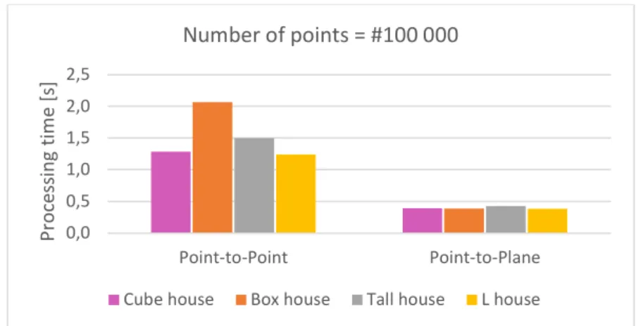
At last, the inlier RMSE and the processing time were tested for other geometries to see if subsampling had the same effect on the geometry. Each point cloud had about 100 000 points and it seams that box house is the only one that doesn’t give a good alignment for ICP point-to-point. The corresponding RMSE is 3,1 cm instead of 0,0 cm as for the others. Figure 11 shows the wrong translation in the x direction after the point-to-point registration. 0 30 60 90 120 150 180 0 10 20 30 40 50 Pro ce ss in g ti me [s ] Maximum iterations [-] Sub1_p2p Sub1_p2l Sub2_p2p Sub2_p2l Sub3_p2p Sub3_p2l 3,0 3,3 3,6 3,9 4,2 10 20 30 40 50 In lie r R MS E [c m] Maximum iterations [-] Sub1_p2p Sub1_p2l Sub2_p2p Sub2_p2l Sub3_p2p Sub3_p2l

7 Figure 11: Effect subsampling on box house after ICP point-to-point

The processing time of ICP point-to-point for the misalignment was also a little bit longer than the others geometries. In general, the performance of both ICP algorithm based on the processing time was equally good, but again ICP point-to-point had a faster processing time. As a result, it is probable that subsampling had little to no effect on the different geometries.

First, St. Marys data set was used to test the influence of rotation on the performance of the ICP algorithms. The axes are shown in Figure 12 to clarify the used terminology for indicating the directions.

Figure 12: The different axes of the St. Marys data set

First, the fine registration algorithms were tested for a random initial rotation (Figure 13) in each direction, to get an impression of the performance.

No rotation Rotation roll-_axis Rotation

pitch-axis Rotation yaw-_axis Figure 13: Different initial rotation angles before the ICP registration is performed (St. Marys)

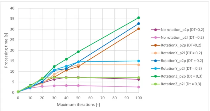
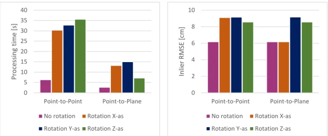
The results on the processing time showed that ICP point-to-point further increases while ICP point-to-point-to-plane stabilizes after 50 maximum iterations. What also stands out is the ease of the algorithm when no initial rotation is involved. Except for the rotation around the x-axis, both algorithms converged eventually to the same inlier RMSE at 100 maximum iterations. It must be noticed that ICP point-to-plane reaches the resulted inlier RMSE earlier with less maximum iterations. Figure 14 compares ICP point-to-point and point-to-plane for each initial rotation, based on the inlier RMSE and the processing time. It illustrates that the inlier RMSE stays the same for both algorithms, except for the initial rotation around x-axis. It may be concluded that both algorithms find it easier to perform a registration without any rotation, which is confirmed by the faster processing time.

Figure 14: Effect of coarse registration on the processing time (above) and the inlier RMSE (bottom) at 100 maximum iterations after fine registration

The effect of rotation on the accuracy was also tested using the GT of the St. Marys data set to understand how accurate the algorithm performed according to the different axes. First, seven points, in particular the centre of the model and a point translated 8m in each direction, were added in the as-built point cloud to allow the evaluation after the registration. Then, the GT was rotated gradually using the transformation matrix to create different initial positions for the as-built point cloud. While creating these alignments, special attention was given to match both the centre of the rotated as-built and the GT as-built, since the origin in CloudCompare differs from the centre of the data set. An example of different rotations around the pitch-axis is given in Figure 15 and the purple points are the added points to the GT.

Figure 15: Example of creating initial alignments for the evaluation of rotation

The outputs of the script were the registered as-built point clouds and they were then compared in CloudCompare against the GT. The differences in distance of the centres and the differences in rotation are measured in CloudCompare using the flowchart presented in Figure 16.

0 10 20 30 40 Point-to-Point Point-to-Plane Pro ce ss in g ti me [s ] No rotation Rotation X-as Rotation Y-as Rotation Z-as 0 2 4 6 8 10 Point-to-Point Point-to-Plane In lie r R MS E [c m] _{No rotation} Rotation X-as Rotation Y-as Rotation Z-as

8 Figure 16: Flowchart of the comparison against the GT

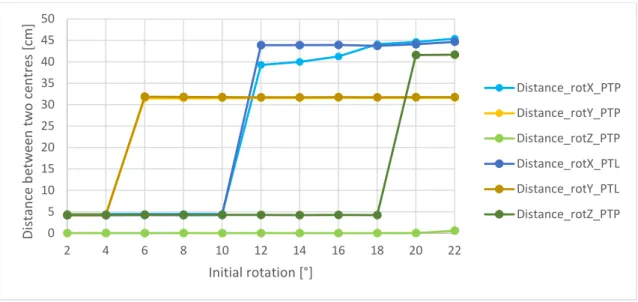
The first experiments test the effects of an initial rotation around the roll-axis, while limiting the maximum iterations to 100. Each situation is evaluated by the displacement in the x, y and z direction and by the final rotation around each axis. The trend of these charts can be summarised by showing the distance in 3D (Figure 17) and the resulted angle (Figure 18). It can be concluded that the point-to-point and point-to-plane show similar results for the rotation around the roll-axis, but the initial rotation can not be more than 10° for both algorithms. Different from the results of the roll-rotation, the pitch-rotation can maximum be four degrees in the initial position. For both ICP-algorithms the initial yaw-rotation should be maximum 18 degrees. Both of the ICP-algorithms show similar results in all situations. These fine registration algorithms are the most sensitive for a pitch-rotation (maximum 4 degrees) and the least sensitive for a yaw-rotation (maximum 18 degrees). The results must be interpreted with caution, because ICP algorithms converge to a local minimum, as it could be depending on the used data set.

Figure 17: Effect of an initial rotation on the distance between the centres (St. Marys)

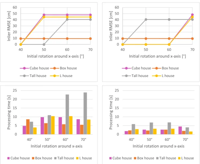
Figure 18: Effect of an initial rotation on the final rotation (St. Marys) To test the result in a perfect situation, the same experiments were done for L house. The results indicate that ICP point-to-point performed well until the initial reached the x-rotation of 40°, the y-rotation of 90° and the z-rotation of 60°. In contrast, the ICP point-to-plane worked until it reached the x-rotation of 60°, the y-rotation of 100° and the z-rotation of 60°. Further, the results show that when the limitation of initial rotation had been reached, the inlier RMSE increased significantly. The visual check suggests that the bad inlier RMSE is caused by a wrong resulted angle.

The limits for the initial rotations, obtained by the tests on the data set L house, were tested for different geometries. Different results were obtained for the initial rotation around the x-axis from 40° to 70°. ICP point-to-point registrations showed some wrong alignments for box house which is rotated around the y-axis, while cube house and tall house are rotated around the x-axis. The results were similar for ICP point-to-plane. The geometry data sets were also evaluated for an initial rotation around the y-axis from 90° to 110°. Also two wrong registrations for specific initial alignments existed and the results are similar for both algorithms. At last the different data sets were tested for rotation angles 60° and 70° around the z-axis. From the results it is noticeable that the resulted inlier RMSE is exceptionally high for both algorithms for L house with an initial rotation of 70°. In contrary with the other geometries, L house’s results stand out for both the processing time and the inlier RMSE. The final registration of cube house and tall house at 60° and 70°. Both have the same problem of being rotated around the z-axis.

The effect of coarse registration on the fine registration was first tested with a little initial rotation (2°) on data set little house and for different geometries. As expected both algorithm were faster after a good coarse registration, but ICP point-to-point is faster in each situation. The trend of inlier RMSE and reveals that ICP point-to-point dropped right away instead of ICP point-to-point, which needed some more time to convergence. Eventually, both variants converged to a same result, see Figure 19. The initial alignment of a good coarse registration.

Make the centres of both point clouds accessible

Select both centres using the point picking tool and write down the differences in x, y and z

Register the original registered as-built point cloud to the GT point cloud by using a manual alignment

followed by the fine registration tool

Write down the angle and calculate the angles in each direction 0 10 20 30 40 50 0 2 4 6 8 10 12 14 16 18 20 22 24 Di stan ce b etw ee n tw o c en tr es [c m] Initial rotation [°] Distance_rotX_PTP Distance_rotY_PTP Distance_rotZ_PTP Distance_rotX_PTL Distance_rotY_PTL Distance_rotZ_PTP 0 2 4 6 8 10 12 14 2 4 6 8 10 12 14 16 18 20 22 R es u lti n g d iff ere n ce in d eg re es [ °] Initial rotation [°] Rotation_rotX_PTP Rotation_rotY_PTP Rotation_rotZ_PTP Rotation_rotX_PTL Distance_rotY_PTL Rotation_rotZ_PTP

9 Figure 19: Effect coarse registration on processing time (above) and

inlier RMSE (bottom) of ICP on Little house at 100 maximum iterations

Now, the effect of coarse registration with a little rotation on different geometries is discussed. What stands out is that inlier RMSE has a general result of 0,0 cm except in three cases. The reason is likely to be the geometry. Tall house and cube house are rotated about 45° whereas box house is translated in the x direction.

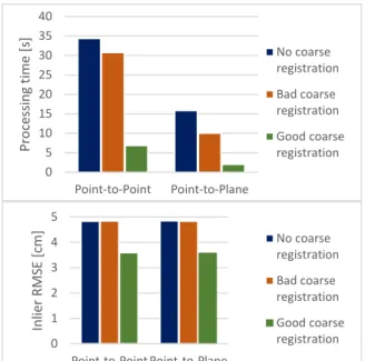
Second, the effect of coarse registration with a bigger initial rotation of 30° was first tested on the data set St. Marys and then for different geometries. Both were compared with the same initial alignment for each situation. Figure 20 gives a visual representation of each created coarse alignment in CloudCompare. Situation 1: no coarse registration Situation 2: bad coarse registration Situation 3: good coarse registration Figure 20: Initial alignment of the St Marys dataset to test the effect of coarse registration

Results illustrates that in each situation the inlier RMSE is the same for both algorithms but that ICP point-to-point is faster. The same trends are noticeable from Figure 19.

Next, the performance of ICP on the data sets geometry is evaluated for the same initial alignments of St Marys. There was no significant difference for ICP point-to-plane whereas for ICP point-to-point the processing time for a good coarse decreased in each situation compared to no and bad coarse registration. In certain situations ICP finds it difficult to handle geometry and it sometimes results in misalignments. For example box house is rotated around y-axis, cube house and tall house are rotated around z-axis.

The effect of missing elements were first tested on the data set St. Marys from which different construction parts were cut in CloudCompare. The resulted point clouds are presented in Figure 21.

Figure 21: Overview of the St. Marys as-built point cloud, adapted to test the effect of missing construction elements

The results of both ICP algorithms were compared and it seems that the effect of missing elements has a positive effect on the processing time, which might be explained by the lower amount of point in the point clouds. Nevertheless, the inlier RMSE slightly increased for both algorithms when elements are missing.

The effect of missing elements was also tested and compared for different geometries. Again some construction elements were missing. The buildings are classified as in 25%, 50%, 75% and 100% complete. The evaluation for cube house and box house indicated that the ICP point-to-point registration failed or did not do a good job. Box house was translated in both x and z direction after only 25% is build, but while the construction progresses the box house is after 75% only translated in x direction. At 50%, the geometry has changed in such way that the ICP point-to-point registration succeed. Cube house is also translated in the x direction at 25% but then as construction process progresses the registration gives better results. In construction progress monitoring this might result in varying results in accuracy as the geometry of the building continuously changes. In addition, the trend of ICP point-to-plane of being faster than ICP point-to-point has also been observed here.

The effect of noise was tested on the data set sports hall with different levels of noise tested for two different initial alignments e.g. bad and good coarse alignment. Each different situation is evaluated on processing time and accuracy over different values of maximum iterations. What stands out is that the processing time for both ICP algorithms is much lower after a good initial alignment, which confirmed the results for testing the effect of the coarse registration. When both algorithms were compared, it was expected that point-to-plane has a lower computation time than point-to-point. Results also revealed that the point clouds with much noise had a much longer processing time than point clouds without noise. Clearly ICP point-to-plane was faster than ICP point-to-point, and a good initial alignment had a great benefit. Even after looking at the resulted inlier RMSE, it may be concluded that a good initial alignment is essential for an accurate result. Comparing the inlier RMSE for both ICP algorithms it may be concluded that they both can handle noise after a good coarse alignment.

The last experiment was conducted to test different scripts for ICP point-to-point. ICP from the library open3D was used in this evaluation, although some other versions of ICP are available. To compare the open3D version against ICP from other sources, one simple situation was tested and 100 is chosen as the limit of maximum iterations for all three algorithms. To compare the three ICP algorithms, all registered point clouds are opened in CloudCompare. The transformation matrices, which are the standard output after performing a registration, show some differences that were noticeable when analysing the transformation matrices. The values of Open3D and PCL are almost the same in contrary to CloudCompare.

To compare the accuracy the six surrounding points are compared to the GT, which was used as an as-planned point cloud in the registration process. The distances between those points are shown in Figure 22 and the first point is on top of the

0 5 10 15 20 25 30 35 40 Point-to-Point Point-to-Plane Pro ce ss in g ti me [s ] No coarse registration Bad coarse registration Good coarse registration 0 1 2 3 4 5 Point-to-Point Point-to-Plane In lie r R MS E [c m] No coarse registration Bad coarse registration Good coarse registration

10 building and the second point is at the bottom point. The results

of the comparison show the best results for Open3D, followed by PCL.

Figure 22: Distances between six points (right) of the GT point cloud and the registered point cloud (left) using three different ICP algorithms. Point one is on top and point two is at the bottom.

D. Comparison coarse registration

A comprehensive comparative evaluation is provided of the RANSAC algorithm and the fast global registration algorithm on different data sets, and demonstrates the efficiency of both approaches, in terms of accuracy and computational time.

First, the coarse registration algorithms were tested on real data using the St. Marys data set. The same initial situation was tested twenty times to check how the algorithms performed. The results were disappointing, leading to a modified test by cutting the floor from the as-planned point cloud. Since the results of the coarse registration differed a lot, box plots were chosen to illustrate the results. Figure 23 represents the amount of inliers for each situation. Cutting the floor had the biggest impact on the fast global registration, because it resulted in a better percentage of inliers. Similar for the processing time, cutting the floor improved the results for the fast global registration and are illustrated in Figure 24.

Figure 23: The variation of inlier RMSE for the St. Marys data set for two situation: with or without the as-planned floor

Figure 24: The variation of processing time for the St. Marys data set for two situation: with or without the as-planned floor

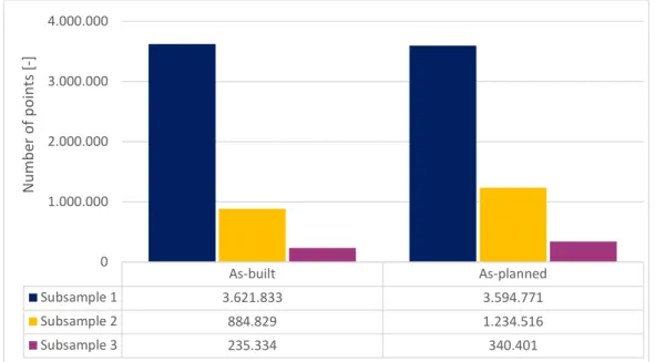
The effect of subsampling was tested using a theoretical point cloud of the L house data set as the processing time of the previous test was very long. For this experiment the exact same point cloud was used for both the as-built and the as-planned point cloud to eliminate other influences. An overview of the different classes is given in Table 3.

Table 3: Number of points of the subsampled data set of L house #400 401 175 points #200 201 177 points #100 100 194 points #50 51 007 points #25 24 948 points

It seems that subsampling had no effect on the inlier RMSE, while it had a huge impact on the processing time for both algorithms. The trend of processing time is illustrated in Figure 25 and Figure 26. Note that the vertical axes differ for the two algorithms. In general, Fast global is as expected much faster than RANSAC.

Figure 25: The effect of subsampling on the inliers RMSE using RANSAC ) on a theoretical point cloud

Figure 26: : The effect of subsampling on the processing time using RANSAC (above) and Fast Global Registration (under) on a theoretical point cloud

Point D_PCL [cm] D_Open3D [cm] D_CC [cm] Point 1 0,0172 0 1,3164 Point 2 0,0167 0 1,1010 Point 3 0,0061 0 0,6367 Point 4 0,0179 0 1,4478 Point 5 0,0053 0,0001 0,4852 Point 6 0,0164 0 0,9556 Mean 0,013267 0,0000 0,9905 0 1000 2000 3000 RANSAC Pro ce ss in g ti me [s ] #25 #50 #100 #200 #400

Number of points after subsampling (*1000):

0 4 8 12 16 20 Fast Global Pro ce ss in g ti me [s ] #25 #50 #100 #200 #400

11 As a result, only subsampled point clouds were used in

subsequent experiments to improve the efficiency.

It might be difficult for some specific geometries to enable a good coarse registration. Therefore, different geometries were tested for inlier RMSE and processing time. The amount of inliers and therefore the inlier RMSE, was higher for RANSAC in all cases. For the processing time of both algorithms a same trend was noticed, but the time interval is much longer for RANSAC. In addition, the angles in all tested point clouds were measured since that is the most important parameter for fine registration. The expected behaviour was having troubles in the yaw-direction due to the geometry. Although the difficulty was created in the yaw-direction, RANSAC created some upside down alignments, which are represented by the outliers in the pitch and roll direction. For a distinct geometry (L house) RANSAC performed better in accuracy, but it needs too much time.

The effect of missing points was first tested using the theoretical data set L house for missing points (Figure 27). The first theoretical situation represents missing points by objects that blocked the visibility and one wall was missing in the first cut and two walls were missing in the second cut. Good results for RANSAC and it is probable that fast global registration is more sensitive to missing points. In terms of speed, the effect of missing elements differed for the algorithms. The processing time of RANSAC was reduced and it could be explained by the smaller number of points. On the other hand, the processing time of fast global increases, but nevertheless the processing time was much longer for RANSAC.

100 %

complete 50% complete 25% complete

Figure 27: Overview of used point clouds to test the effect of missing points

Then, the same test was performed using only missing construction elements (Figure 28) to analyse if the behaviour of the algorithm to geometry. By cutting of the roof, the point cloud was reduced to 75%. The other point clouds further reduced the amount of points by cutting walls.

100% complete 75% complete 50% complete 25% complete Figure 28: An overview of the used data sets to test the effect of missing elements

Then, the effect of missing construction elements was also tested on a real situation using the data set St. Marys. The different missing elements are presented in Figure 21 but were more subsampled for computation reasons. The inlier RMSE and the percentage inliers indicated that fast global almost certainly performed worse in situations of missing construction

elements, because the amount of inliers reduced when cutting construction elements. On contrary to the theoretical point clouds, the processing time of fast global and RANSAC followed the same trend.

The effect of noise was tested on subsampled point clouds from the data set sports hall. The point clouds were subsampled to the same amount of points, but different levels of noise. An overview of the used point clouds is given in Figure 29.

Much noise 50 000 points Less noise 50 000 points No noise 50 000 points Figure 29: Visuals of the used as-built point clouds with different levels of noise

Each situation was tested ten times and the variation of the amount of inliers. Figure 31 shows the inlier RMSE and by combining both results, it may be concluded that both the algorithms can handle noise. In addition, the noise had no significant effect on the processing time for both algorithm, although Fast Global was each time much faster.

Figure 30: The percentage of inliers for three situation: much, less and no noise (Sports hall)

Figure 31: The variation of the inlier RMSE for three different situations: much, less and no noise (Sports hall)

12 IV. CONCLUSION

In this research, it has been explained that despite various data acquisition methods and approaches, the success is limited and the development of automated systems for construction progress monitoring and evaluation has not yet reached the required efficiency and reliability to be applied by the construction industry. Therefore, a comparative evaluation, based on accuracy and efficiency, of two fine and two coarse registration techniques was performed to evaluate the effectiveness and to gain a detailed understanding of factors that effect the performance evaluation. However, this method may involve potential measurement error. A major problem with experimental data is that it does represent the results for the real world applications.

The framework we developed is suitable for each registration technique described in this paper with a limited time budget, while at the same time providing accurate robust estimation. The research would have been more interesting if more algorithms could have been included and compared to obtain further in-depth information. There are certain problems with the use of some existing algorithm. One of these is that they are not easily find or can not easily applied due to different programme languages and another is that there are less algorithms available on open sources. This needs a better knowledge of programming.

However, this research does not fully explain the effect of translation on the fine registration method, because only samples were taken. In the evaluation of the coarse registration algorithms, it seemed that subsampling had an impact on the fast global registration algorithm when real data was used. This could be further researched. Moreover, further research could test the algorithms on a larger data set and could compare the variants against the original algorithm.

REFERENCES

[1] A. Braun, S. Tuttas, U. Stilla, and A. Borrmann, "Incorporating knowledge on construction methods into automated progress monitoring techniques," in The 23rd International Workshop of the European Group for Intelligent Computing in Engineering, Krakow, Poland, 2016.

[2] Q. Wang, Y. Tan, and Z. Mei, "Computational Methods of Acquisition and Processing of 3D Point Cloud Data for Construction Applications," Archives of Computational Methods in Engineering, vol. 27, no. 2, pp. 479-499, Apr 2020, doi: 10.1007/s11831-019-09320-4.

[3] S. Alizadehsalehi and I. Yitmen, "The Impact of Field Data Capturing Technologies on Automated Construction Project Progress Monitoring," World Multidisciplinary Civil Engineering-Architecture-Urban Planning Symposium 2016, Wmcaus 2016, vol. 161, pp. 97-103, 2016, doi: 10.1016/j.proeng.2016.08.504. [4] Y. Xua, R. Boernera, W. Yaoa, L. Hoegnera, and U. Stillaa,

"Automated coarse registration of point clouds in 3D urban scenes using voxel based plane constraint," ISPRS Annals of the Photogrammetry, Remote Sensing and Spatial Information Sciences, vol. IV, 2/W4, p. 7, 2017, doi: 10.5194/isprs-annals-IV-2-W4-185-2017.

[5] X. Gu, X. Wang, and Y. Guo, "A Review of Research on Point Cloud Registration Methods," presented at the IOP Conference Series: Materials Science and Engineering, 2020. [Online]. Available: https://iopscience.iop.org/article/10.1088/1757-899X/782/2/022070.

[6] L. Cheng et al., "Registration of Laser Scanning Point Clouds: A Review," Sensors, vol. 18, no. 5, May 2018, Art no. 1641, doi: 10.3390/s18051641.

[7] F. Tombari and F. Emondino, "Feature-based automatic 3D registration for cultural heritage applications," Marseille, France, 2013.

[8] H. Kim and A. Hilton, "Evaluation of 3D Feature Descriptors for Multi-modal Data Registration," (in English), 2013 International

Conference on 3d Vision (3dv 2013), Proceedings Paper pp. 119-126, 2013, doi: 10.1109/3dv.2013.24.

[9] Y. Xian, J. Xiao, Y. Wang, M. Shan, and C. Zhou, "A Review of Fine Registration for 3D Point Clouds," Proceedings of the 2016 5th International Conference on Advanced Materials and Computer Science, vol. 80, pp. 108-113, 2016 2016.

[10] Y. Diez, F. Roure, X. Llado, and J. Salvi, "A Qualitative Review on 3D Coarse Registration Methods," (in English), Acm Computing Surveys, Review vol. 47, no. 3, p. 36, Apr 2015, Art no. 45, doi: 10.1145/2692160.

[11] B. Bellekens, V. Spruyt, R. Berkvens, and M. Weyn, "A Benchmark Survey of Rigid 3D Point Cloud Registration Algorithms," presented at the AMBIENT 2014: The Fourth International Conference on Ambient Computing, Applications, Services and Technologies, Rome, 2015, ISBN: 978-1-61208-356-8.

[12] H. Mahami, F. Nasirzadeh, A. H. Ahmadabadian, and S. Nahavandi, "Automated Progress Controlling and Monitoring Using Daily Site Images and Building Information Modelling," Buildings, vol. 9, no. 3, Mar 2019, Art no. 70, doi: 10.3390/buildings9030070.

[13] Z. Pucko, N. Suman, and D. Rebolj, "Automated continuous construction progress monitoring using multiple workplace real time 3D scans," Advanced Engineering Informatics, vol. 38, pp. 27-40, Oct 2018, doi: 10.1016/j.aei.2018.06.001.

[14] R. Maalek, D. D. Lichti, and J. Y. Ruwanpura, "Automatic Recognition of Common Structural Elements from Point Clouds for Automated Progress Monitoring and Dimensional Quality Control in Reinforced Concrete Construction," Remote Sensing, vol. 11, no. 9, May 2019, Art no. 1102, doi: 10.3390/rs11091102.

[15] Q. Wang, J. J. Guo, and M. K. Kim, "An Application Oriented Scan-to-BIM Framework," Remote Sensing, vol. 11, no. 3, Feb 2019, Art no. 365, doi: 10.3390/rs11030365.

[16] T. Nuttens, V. De Breuck, R. Cattoor, K. Decock, and I. Hemeryck, "Using BIM Models for the design of large rail infrastructure projects: Key factors for a successful implementation," in Building information systems in the construction industry, 2018.

[17] A. Braun, S. Tuttas, A. Borrmann, and U. Stilla, "Automated progress monitoring based on photogrammetric point clouds and precedence relationship graphs," in The 32nd International Symposium on Automation and Robotics in Construction and Mining, Oulu, Finnland, 2015.

[18] S. Tuttas, A. Braun, A. Borrmann, and U. Stilla, "Acquisition and Consecutive Registration of Photogrammetric Point Clouds for Construction Progress Monitoring Using a 4D BIM," Pfg-Journal of Photogrammetry Remote Sensing and Geoinformation Science, vol. 85, no. 1, pp. 3-15, Feb 2017, doi: 10.1007/s41064-016-0002-z.

[19] R. Becker et al., "BIM - towards the entire lifecycle," International Journal of Sustainable Development and Planning, vol. 13, no. 1, p. 11, 2018, Art no. 707833, doi: 10.2495/SDP-V13-N1-84-95. [20] L. Lei, Y. Zhou, H. Luo, and P. E. D. Love, "A CNN-based 3D

patch registration approach for integrating sequential models in support of progress monitoring," Advanced Engineering Informatics, vol. 41, Aug 2019, Art no. Unsp 100923, doi: 10.1016/j.aei.2019.100923.

[21] M. Murphy and C. Dore, "Semi-automatic generation of as-built BIM façade geometry from laser and image data," Information Technology in Construction, vol. 19, pp. 20-46, 2014.

[22] M. Bueno, F. Bosche, H. Gonzalez-Jorge, J. Martinez-Sanchez, and P. Arias, "4-Plane congruent sets for automatic registration of as-is 3D point clouds with 3D BIM models," Automation in Construction, vol. 89, pp. 120-134, May 2018, doi: 10.1016/j.autcon.2018.01.014.

[23] D. Rebolj, Z. Pucko, N. C. Babic, M. Bizjak, and D. Mongus, "Point cloud quality requirements for Scan-vs-SIM based automated construction progress monitoring," Automation in Construction, vol. 84, pp. 323-334, Dec 2017, doi: 10.1016/j.autcon.2017.09.021. [24] O. Moselhi, H. Bardareh, and Z. Zhu, "Automated Data Acquisition in Construction with Remote Sensing Technologies," (in English), Applied Sciences-Basel, Review vol. 10, no. 8, p. 31, Feb 2020, Art no. 2846, doi: 10.3390/app10082846.

[25] H. Hamledari, B. McCabe, S. Davari, and A. Shahi, "Automated Schedule and Progress Updating of IFC-Based 4D BIMs," (in English), Journal of Computing in Civil Engineering, Article vol. 31, no. 4, p. 16, Jul 2017, Art no. 04017012, doi: 10.1061/(asce)cp.1943-5487.0000660.

[26] J. Tulke and J. Hanff, "4D construction sequence planning - new process and data model," presented at the CIB-W78 24th International Conference on Information Technology in Construction, 2007.