Stabilising greenhouse gas concentrations at low levels: an assessment of options and costs

(1)

Netherlands Environmental Assessment Agency (MNP), P.O. Box 303, 3720 AH Bilthoven, the Netherlands; Tel: +31-30-274 274 5; Fax: +31-30-274 4479; www.mnp.nl/en

MNP Report 500114002/2006

Stabilising greenhouse gas concentrations at low levels: an assessment of options and costs

D.P. van Vuuren, M.G.J. den Elzen, P.L. Lucas, B. Eickhout, B.J. Strengers, B. van Ruijven, M.M. Berk, H.J.M. de Vries,

M. Hoogwijk*, M. Meinshausen**, S.J. Wonink, R. van den Houdt, R. Oostenrijk

* : Ecofys BV, Utrecht, the Netherlands

**: Potsdam Institute for Climate Impact Research (PIK), Postdam, Germany

Contact:

Detlef P. van Vuuren KMD

detlef.van.vuuren@mnp.nl

This investigation has been performed within the framework of S/550025 Methods for Sustainability Analysis

(2)

Parts of this publication may be reproduced, on condition of acknowledgement: 'Netherlands Environmental Assessment Agency, the title of the publication and year of publication.'

(3)

Preface

This report presents the results of an extensive research project on the potential for stabilising greenhouse gas concentration in the atmosphere at relatively low levels in order to reduce climate change risks. Most studies so-far have concentrated on higher stabilisation levels, but given new insights in the science of climate change, these might not be anymore sufficient to achieve the overall target of the UN Framework Convention on Climate Change (prevent dangerous antropogenic climate change). The results of this research project have been reported in seven related articles. Four of these articles focus on potentials to reduce greenhouse gas emissions. One article focuses on the required emission reduction rates for different stabilisation levels, and finally, two articles look into the integrating aspects of the project and report results for the world and separate regions. The research has been done using MNP’s Environmental Integrated Assessment modelling framework IMAGE 2.3 and the related models IMAGE/TIMER (an energy systems model) and FAIR (a climate policy evaluation tool). The seperate articles have been submitted to various journals. The purpose of this report is to bring the results together – both for documentation purposes and to provide readers a complete and comprehensive overview of latest insights in various aspects of low concentration stabilisation mitigation scenarios.

While the chapters in this report focus on climate mitigation options, it is acknowledged that this is only part of the story. First of all, adaptation to climate change impacts forms an important part of climate policy, as a substantial level of change has already become

inevitable. Moreover, the climate change problem is to be considered part of the broader issue of sustainable development. Solutions to the climate problem will need to fit in with

sustainable development, both to avoid creating new problems while dealing with climate change, to seize opportunities for synergies with meeting other policy objectives, and to render societal support for the implementation of climate policies. Also the way society developes will influence the challenge of mitigating climate change. This broader context is partly addressed n some of the chapters e.g. by looking at the implications of options for land use and synergies with air pollution abatement (co-benefits), and by exploring the influence of baseline developments (scenarios) on the feasibility and costs of climate change

mitigation. These issues will be the subject of future research.

The results of the projects as a whole have also be summarised in a concise report also available from MNP (www.mnp.nl)

(4)

(5)

Abstract

Stabilising greenhouse gas concentrations at low levels: an assessment of options and costs

Preventing ‘dangerous antropogenic interference of the climate system’ may require

stabilisation of greenhouse gas concentrations in the atmosphere at relatively low levels such as 550 ppm CO2-eq. and below. Relatively few studies exist that have analysed the

possibilities and implications of meeting such stringent climate targets. This report presents a series of related papers that address this issue – either by focusing on individual options or by presenting overall strategies at the global and regional level. The results show that it is

technically possible to reach ambitious climate targets – with abatement costs for default assumptions in the order of 1-2% of global GDP. To achieve these lower concentration levels, global emissions need to peak within 15-20 years. The stabilisation scenarios use a large portfolio of measures, including energy efficiency but also carbon capture and storage, large scale application of bio-energy, reduction of non-CO2 gasses, increased use of

renewable and/or nuclear power and carbon plantations.

Key words:

(6)

(7)

Rapport in het kort

Stabilisatie van broeikasgasemissies op lage niveau’s: een studie naar de mogelijkheden en kosten

Het voorkomen van ‘gevaarlijke menselijke beïnvloeding van het klimaatsysteem’ vereist mogelijk de stabilisatie van broeikasgasconcentraties in de atmosfeer op relatief lage niveau’s (zoals 550 ppm CO2-eq. en lager). In de literatuur zijn er nauwelijks studies beschikbaar die

op een geïntegreerde wijze hebben gekeken naar de mogelijkheden voor en gevolgen van het bereiken van dergelijke ambitieuze klimaatdoelstellingen. Dit rapport bevat een serie

gerelateerde artikelen die op dit onderwerp ingaat – enerzijds door naar de mogelijke bijdrage van individuele mitigatieopties te kijken en anderzijds door analyses van geïntegreerde strategieën op mondiaal en regionaal niveau. De resultaten laten zien dat het technisch mogelijk is om aan ambitieuze klimaatdoelen te voldoen – met reductiekosten onder standaard aannames in de orde van 1-2% van het mondiale bruto nationale produkt (BNP). Daartoe dienen de mondiale emissies wel binnen 15-20 jaar hun maximumniveau te bereiken. De scenario’s tonen aan dat een brede portfolio van opties noodzakelijk is, inclusief

verbetering van de energie-efficientie, CO2-afvang-en-opslag, grootschalige benutting van

bio-energie, terugdringen van niet-CO2 broeikasgassen, meer benutting van hernieuwbare

en/of nucleaire energie en het toepassen van koolstofplantages.

Trefwoorden:

(8)

(9)

Summary

Avoiding dangerous anthropogenic interference with the climate system may require stabilisation of greenhouse gas concentrations in the atmosphere at relatively low levels. Current studies on emission pathways, for instance, indicate that in order to achieve the EU 2oC climate target with a probability larger than 50% may require stabilisation below 450 ppm CO2-eq. Unfortunately, the number of multi-gas stabilisation scenarios currently

available in scientific literature exploring strategies to stabilise greenhouse gas concentration at such low levels or even at 550 ppm CO2-eq. is severely limited. As a result, information

about how to achieve these levels is mostly lacking.

In this study, we have used the IMAGE integrated assessment modelling framework, including its world energy model TIMER and the climate policy support model FAIR– SiMCaP to explore the environmental and economic effects of mitigation scenarios stabilising long-term greenhouse gas concentrations at 650, 550 and 450 ppm CO2-eq.

(compared to current literature 450 and 550 are low concentration levels; 650 is a medium stabilisation level and is added for comparison). The main research question of this study was whether and how low levels of stabilisation of greenhouse concentrations can be reached and at what costs. It focused on three different subquestions:

What would be the required level of emission reductions needed to stabilise greenhouse gas concentration levels at 650, 550 and 450 ppm CO2-eq. on the

long-term?

What technical potential is available to abate future greenhouse gas emissions, in particular by reducing non-CO2 gasses, growing carbon plantations (sinks), use of

renewables and use of hydrogen as a secondary energy carrier?

What cost-effective portfolios of reduction measures could achieve stabilisation at 650, 550 and 450 ppm CO2-eq. and what could be the abatement costs and climate

and air-pollution benefits of these portfolios, both at the global and regional level? The research was published as separate articles. This publication combines these articles in one single report.

1. Development without climate policies

In the study, updated versions of the Special Report on Emission Scenarios (SRES) scenarios of the Intergovernmental Panel on Climate Change (IPCC) were used. These updates

included new insights in population trajectories (lower for each scenario), updated GDP trajectories (high economic rates in some developing regions take a long time to build up), revised energy resources (a downward revision of oil and natural gas resources) and new modeling tools (TIMER 2.0 was used as energy model). The B2 scenario, used as central baseline in the study, is developed on the basis of the International Energy Agency’s (IEA)

(14)

2004 energy projection and the marker B2 IPCC scenario and and forms a medium emission scenario. The B1 and A1b scenario are used as low- and high emission alternatives.

Without climate policies, the scenarios explored show greenhouse gas emissions

to increase significantly. In the B2 scenario, emissions increase from about

10 GtC-eq. today to around 23 GtC-eq. in 2050 and more-or-less stabilise at this level afterwards. Compared to other studies this can be regarded as a medium estimate. The scenario results in greenhouse gas concentration in 2100 of above 900 ppm CO2-eq.

This implies that significant emission reduction is needed to stabilise concentration at the range 450-650 ppm CO2-eq. The alternative A1b and B1 scenarios show higher,

respectively lower emissions resulting from assumptions on a) higher economic growth and more energy intensive life-styles (A1) and b) sustainable development policies (B1). The B1 scenario leads more-or-less to a 650 ppm CO2-eq. stabilisation

level – but should certainly not be regarded as policy-free (as it assumes improved energy efficiency and increased use of renewable energy, but for other reasons than climate policy).

2. Pathways to stabilisation targets

Using the policy support model FAIR–SiMCaP, the study explored pathways for stabilising greenhouse gas concentrations at 450, 550 and 650 ppm taking into account uncertainties and inertia in both the climate system and the social-economic system. The emission pathways are calculated on the basis of a cost-optimal implementation of available reduction options. The main findings are:

There is no single clear pathway that leads to a particular stabilisation level. Instead, there is a broad envelope of pathways containing pathways that lead to stabilisation, depending on early action or delayed mitigation action (or in between). The pathways within the envelope have almost the same probability to meet

temperature targets. The 550 and 650 ppm CO2-eq. stabilisation pathways always stay

below the target concentrations. For 450 ppm CO2-eq. pathways unavoidably first

overshoot the target level and only return to the stabilisation level after 2100. The costs of the envelopes show a wide range, depending on early-action or

delayed response. The delayed response pathway shows lower costs in the

short-term, but in long-term the costs are higher. The early action pathways benefit from the induced technology development and the early signal to the energy system.

Comparing the discounted cumulative costs, shows that at discount rates of 4-5% or less early pathways lead to lowest costs.

The ranges of emissions pathways for the 450 ppm CO2-eq. and 550 ppm CO2

-eq. are relatively tight. Meeting both concentration targets requires strong

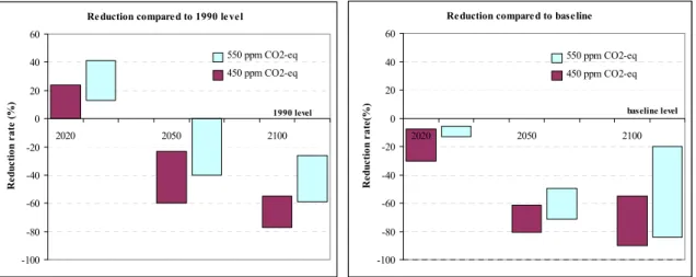
emission reductions in the short-term. For 550 ppm CO2-eq, global emissions needs

to be peak by 2025 – and then decrease rapidly. For the 450 ppm CO2-eq. scenario

(15)

1 summarizes the required reduction rates compared to 1990 levels and compared to baseline for the lowest two levels (450 and 550 ppm).

Emission reductions depicted for 450 and 550 ppm CO2-eq. require early participation of major greenhouse gas emittors, including developing countries.

The emission reductions calculated for the different profiles in the next 20-30 years cannot be achieved by a small group of countries only. This will somehow require a broadening of developed and developing country participation in international policy regimes for the mitigation of greenhouse gases.

Reduction compared to 1990 level

-100 -80 -60 -40 -20 0 20 40 60 2020 2050 2100 R edu ct io n r at e (% ) 1990 level 450 ppm CO2-eq 550 ppm CO2-eq

Reduction compared to baseline

-100 -80 -60 -40 -20 0 20 40 60 2020 2050 2100 R edu ct io n r at e( % ) _{baseline level} 450 ppm CO2-eq 550 ppm CO2-eq

Figure S-1 Emission reduction levels required for stabilisation at 450 and 550 ppm CO2-eq.

The ranges presented are a function of the timing of reductions (particularly important for left side figure) and baseline emissions (in particular important for right side figure)

3. Studies on abatement potential

In preparation of the overall assessment of greenhouse gas abatement potential, separate analysis was performed into abatement potential of specific options, i.e. carbon plantations (sinks), non-CO2 greenhouse gas emission reduction, renewable energy and the role of

hydrogen.

Potential to sequester carbon dioxide by carbon plantations

One way to reduce greenhouse gas concentration levels is to sequester carbon dioxide by means of carbon plantations. Our analysis leads to the following conclusions:

Carbon plantations can theoretically sequester around 1-2 GtC annually

depending on baseline developments and other uncertainties. In the B2 scenario,

the carbon sequestration potential on abandoned agricultural land increases from 60 MtC/yr in 2010 to 2700 MtC/yr in 2100, assuming that forests are harvested and used to meet the timber demand. The cumulative amount is 118 GtC. The largest contributors in the coming 20 years are South Africa and Russia. By the end of the century, the lead is taken over by China and South America. The cumulative

(16)

sequestration potential goes from 17 GtC in the A2 scenario to 148 GtC in the A1b scenario, and strongly depends on the amount of abandoned agricultural land. Carbon plantations provide a relatively low cost mitigation option. Taking into

account the main costs components, i.e. land and establishment costs, and not taking into account the revenues from timber sales, the largest part of the potential up to 2025 can be supplied below 100$/tC. Beyond 2050, more than 50% of the costs exceed 200$/tC. Compared to other mitigation options, this is still relatively cheap so a large part of the potential will likely be used in an overall mitigation strategy. However, since huge emission reductions are probably needed, the relative contribution of plantations will be small (around 3%).

The range of supply and costs presented falls well in the range of other (regional

and global) carbon sequestration cost-supply studies. An exception is East Asia,

where the land prices might be too high and where revenues from timber extraction are more important than in other regions.

The largest source of uncertainty is the growth rate of plantations compared to

the natural vegetation. Especially if growth falls short, costs per ton of carbon

strongly increase. A different baseline scenario than B2 has a limited impact on costs per unit of carbon sequestration, suggesting that costs do not strongly depend on the baseline scenario used.

The role of non-CO2 greenhouse gases

Recently, considerable attention has been paid to the contribution of non-CO2 gases to

emission reduction. However, most information on abatement potentials focuses on the short-term. Here, we also explored the long-term potential of non-CO2 greenhouse gases, finding

that:

Over the century, the share of non-CO2 gases in the baseline is likely to drop

from 22% to around 15%, as their growth rate is slower than that of CO2. Non-CO2 gases are mostly coupled to agricultural activities. These activities are strongly

coupled to population growth and population will likely stabilise (or even decline) during the 21st century.

Assumptions about technological change and barriers for implementation play

an important role in the assessment of future contributions of non-CO2 gases in

mitigation scenarios. If the reduction potential for non-CO2 gases is restricted to the

set of reduction measures that have been identified specifically for 2010/2020, the role of non-CO2 gases is limited. Based on a literature survey and expert judgment we

estimate that the potential for the reduction of non-CO2 gases is much larger in the

long-run (up to about 70%).

Including non-CO2 abatement options in strategies aiming at stabilising

greenhouse gas concentrations can reduce costs by about 30% (if cumulated over the century) compared to CO2-only strategies. For pathways for stabilisation at 450 ppm, the share of non-CO2 emission reduction in total abatement is about 75% in

the short term. It decreases to around 15% in 2050 due to the limited potential of non-CO2 reduction and the rapidly increasing global reduction objective. Along with the

fluorinated gases, methane emission reductions from mainly fossil fuel production and landfills form the largest share in total non-CO2 emission reduction.

(17)

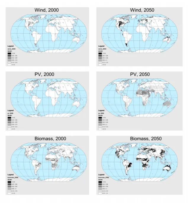
Renewable energy

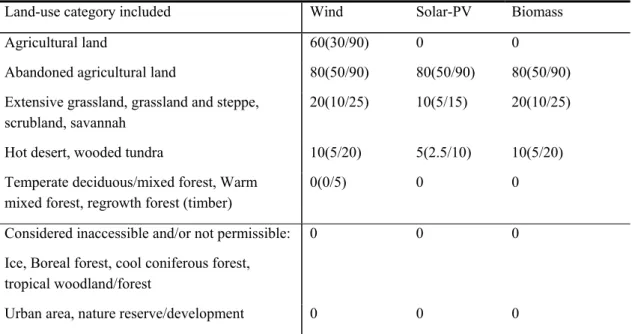
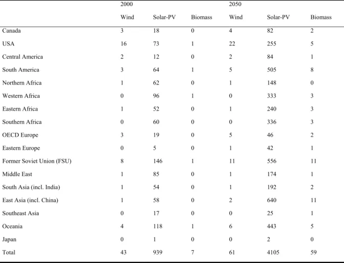
Estimates of the potential contribution of renewable energy (wind, solar,

biomass) to mitigation of greenhouse gas emissions are strongly dependent on underlying assumptions. In the literature, often technical, theoretical, economic or

other potential production levels and costs are mentioned for renewable energy sources. All these categories, however, do strongly depend on assumptions (land, technology, costs etcetera) – and should therefore be used with care.

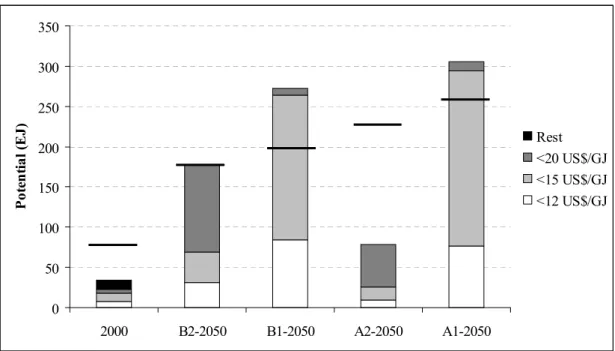
Theoretically, future electricity demand can be easily met by renewable energy

sources in most regions by 2050 at production costs below 10 ¢ kWh-1. Major uncertainties in the estimated worldwide potential of about 200 to 300 PWh yr-1 below this cost level are the degree to which land is actually available and the rate and extent at which specific investment costs can be reduced. In some regions, competition for land among the three options may reduce the combined potential.

The potential to produce liquid biofuels is estimated in the order of

75-300 EJ yr-1. This implies that depending on the scenario, about 50-100% of world

transport demand can be supplied on the basis of bio-energy. However, in that case no bio-energy would be available for use in other sectors (like electricity production).

The role of hydrogen in stabilisation scenarios

• Hydrogen will probably not play an important role before the mid-21st_century

in the world energy system, neither with nor without a climate policy. Thereafter it can become a major secondary energy carrier but only under optimistic assumptions. In our scenarios, which mainly use costs as decisive factor,

high costs as a result of infrastructure, production costs and the price of fuel cells prevent hydrogen penetration in the first half of the century. These cost barriers may disappear in the second half of the century.

• Without climate policy, CO2 emissions from energy systems with hydrogen are likely to be higher than those of systems without hydrogen. In our scenarios,

hydrogen is mainly produced from coal and natural gas (as these form the lowest costs routes). Hence, hydrogen rich scenarios without climate policy increase CO2

emissions up to 30% by 2100 compared to the baseline.

• Energy systems with hydrogen respond more flexibly and at lower marginal

abatement costs to climate policy. The reason for this is related to the previous

conclusion: the use of hydrogen provides new and presumably cheap carbon emission reduction options in the form of centralized Carbon Capture and Storage (CCS). As a result, the costs of reaching a given climate target may be reduced substantially. The combined potential of different options

Taking into account the results of the specific studies on the potential of mitigation options, the study also assessed the influence of various uncertainties on the total mitigation potential related to factors such as 1) baseline developments, 2) different technology assumptions (optimistic/default/pessimistic) and 3) other factors (e.g. societal acceptance of nuclear power). It was found that the total abatement potential ranges from about 60-70% in 2050 to about 80-90% in 2100 from baseline level, for the default baseline scenario (B2).

(18)

0 5 10 15 20 25 30 200 U S$/tC eq 500 U S$/tC eq 1000 US$ /tCeq 200 U S$/tC eq 500 U S$/tC eq 1000 US$ /tCeq E m is si on r edu ct io n ( G tC -e q

) CO2 energy/industry Carbon plantation Non-CO2

2050 2100

Figure S-2 Abatement potential under the B2 scenario at various marginal cost levels (using default assumptions). Horizontal line indicates baseline emissions; comparison of abatement potential and baseline emissions indicates reduction rate.

4. Integrated scenarios

Global results

On the basis of the IPCC B2, A1b and B1 baseline scenarios, mitigation scenarios were developed that stabilise the greenhouse gas concentrations at relatively low stabilisation levels. The analysis takes into account a large number of reduction options, such as reductions of non-CO2 gases, carbon plantations and measures in the energy system.

• The study shows that, technically, stabilising greenhouse concentrations at 650,

550, 450 ppm and, under specific assumptions, 400 ppm CO2-eq. is feasible from

a median baseline scenario on the basis of known technologies. The study shows

stabilisation as low as 450 ppm CO2-eq. to be technically feasible. To achieve these

lower concentration levels, global emissions need to peak within the first two decades. The net present value of abatement costs (2010-2100) for the B2 baseline scenario (a medium scenario) increases from 0.2% of cumulative GDP to 1.1% going from stabilisation at 650 to 450 ppm. On the other hand, the probability of meeting the EU climate target (limit global mean temperature increase to 2oC) increases from 0-10% to 20-70% when going from 650 to 450 ppm. The lowest level of 400 ppm CO2-eq.

can be reached if the option of combining bio-energy and carbon capture and storage is added to the model.

• Creating the right socio-economic and institutional conditions for stabilisation

will represent the single most important step in any strategy towards greenhouse gas concentration (GHG) concentration stabilisation. The types of reductions

described in this paper will require major changes in the energy system, stringent abatement action in other sectors and related large-scale investment in alternative

(19)

technologies. Some of these changes are required on the short term (2020). Creating a sense of urgency will be required to achieve this.

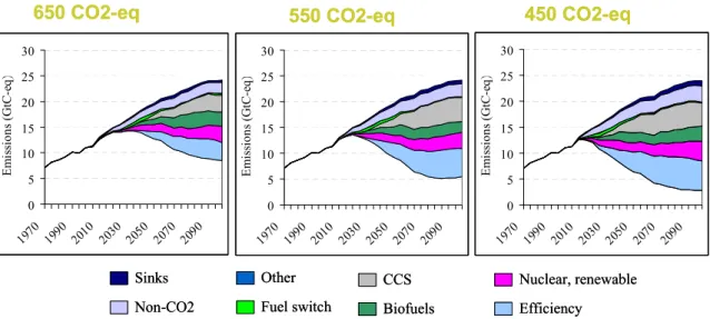
• Strategies consist of a portfolio of measures. There is no magic bullet. Given our

default assumptions, energy efficiency and carbon capture and storage (CCS) contribute significantly to the overall portfolio. All scenarios apply a wide-range of

technologies in reducing emissions. Some technologies, however, contribute more than others. Efficiency plays an important role in the overall portfolio. CCS is another important technology under default assumptions – but may be substituted at limited costs against other zero-carbon emitting technologies in the power sector.

• Uncertainties are important. Uncertainties play an important role in the whole analysis – and thus in decision-making on mitigation strategies. Uncertainties include 1) the required reduction levels, 2) baseline emissions, and 3) availability and costs of different technologies. For a given baseline and target, the uncertainties in costs is at least in the order of 50%, with the most important uncertainties including land-use emissions, the potential for bio-energy and the contribution of energy efficiency. Given this dominant role, it is important to develop strategies that are robust against these uncertainties.

650 CO2-eq _{550 CO2-eq} 450 CO2-eq

0 5 10 15 20 25 30 1970 1990 2010 2030 2050 2070 2090 E m issi on s ( G tC -e q) 0 5 10 15 20 25 30 1970 1990 2010 2030 2050 2070 2090 E m issi on s ( G tC -e q) 0 5 10 15 20 25 30 1970 1990 2010 2030 2050 2070 2090 E m issi on s ( G tC -e q) Sinks Non-CO2 Other Fuel switch CCS Biofuels Nuclear, renewable Efficiency

650 CO2-eq _{550 CO2-eq} 450 CO2-eq

0 5 10 15 20 25 30 1970 1990 2010 2030 2050 2070 2090 E m issi on s ( G tC -e q) 0 5 10 15 20 25 30 1970 1990 2010 2030 2050 2070 2090 E m issi on s ( G tC -e q) 0 5 10 15 20 25 30 1970 1990 2010 2030 2050 2070 2090 E m issi on s ( G tC -e q) Sinks Non-CO2 Other Fuel switch CCS Biofuels Nuclear, renewable Efficiency

Figure S-3 Reduction measures in stabilisation scenarios for 650, 550 and 450 ppm CO2-eq.

Regional results

Finally, the study looked into the regional abatement action and costs using the FAIR model. These mainly depend on 1) the concentration stabilisation level chosen, 2) the (regional) baseline emissions, 3) the distribution of emission reduction efforts (depending on the allocation scheme), and 4) transfers related to international emissions trading. Here, regional costs were explored for two allocation schemes: Multi-Stage, and Contraction &

Convergence, and two stabilisation levels (450 and 550 ppm CO2-eq.). The main findings are:

• To achieve the low CO2-equivalent concentrations, the developed regions need to reduce their emissions substantially below 1990 levels and the developing regions need to make reductions compared to their baseline emissions levels as soon as possible. The developed countries as a group would need to adopt emissions

(20)

reduction targets of 10% to 25% below 1990 levels by 2020 and 60% to 90% below 1990 levels by 2050 in order to stabilise greenhouse gas concentrations at 550 and 450 ppm CO2-equivalent, respectively.

• Under the regimes explored the abatement costs as percentages of Gross

Domestic Product (GDP) vary significantly by region, with high costs for the Middle East &Turkey and the former Soviet Union, medium costs for the OECD countries and low costs or even gains for most non-Annex I regions. Some

developing regions gain from participating in international emissions trading. In addition to the abatement costs, fossil-fuel-exporting regions are also likely to be affected by losses of coal and oil exports. In some regions, however, these could be offset by increased bio-energy export gains.

• Also at the regional scale, abatement strategies to meet low stabilisation targets

require a portfolio of mitigation options. Especially in the former Soviet Union and

the Asia region – but also in other parts of the world, non-CO2 abatement options are

important in the short term in reducing emissions. Carbon capture and storage, energy efficiency improvements, bio-energy use and the use of renewables dominate

(21)

1 Introduction

1.1 Background for exploring low-concentration stabilisation

scenarios

Climate change poses one of the most challenging environmental threats to the world.

According to the Intergovernmental Panel of Climate Change in its Third Assessment Report (IPCC, 2001) mankind has demonstrably changed the earth’s climate system since the pre-industrial era and – without climate policy responses – is likely to changes much further, with expected increases in global temperature in the 2000-2100 period ranging from 1.4 to 5.8 degrees Celsius. Article 2 of the United Nations Framework Convention on Climate Change (UNFCCC) states as its ultimate objective: ‘Stabilization of greenhouse gas (GHG)

concentrations in the atmosphere at a level that would prevent dangerous anthropogenic interference with the climate system’ (UNFCCC, 1992). However, what constitutes a non-dangerous level cannot be unambiguously determined, as this depends on both uncertainties in the cause-effect chain of climate change as well as on political choices about the level of risks viewed acceptable. In its third assessment report (TAR) (IPCC, 2001), the

Intergovernmental Panel on Climate Change (IPCC) identified different dimensions of climate risks also known as ‘reasons for concern’ that could constitute the basis for determining dangerous levels of climate change. It made clear that already with limited temperature increase impacts of climate change could already be severe for some systems or regions (Figure 1.1).

1 2 3 4 5

Risks to unique & threatened systems

Risks to some Risks to many

Increase Large increase Risk of extreme_{weather events}

Distribution of impacts Negative for some regions Negative for most regions Aggregate impacts

Net negative in all metrics Positive or negative monetary;

majority of people adversely affected

Past Future

0 -0.7

Increase in global mean temperature after 1990 (°C)

Very low Higher Risks of large scale_{singularities}

(22)

This finding has been confirmed by more recent research. Some of the recent literature suggests that climate risks could already be substantial for an increase of 1–3oC compared to pre-industrial levels (see O 'Neill and Oppenheimer, 2002;ECF and PIK, 2004;Leemans and Eickhout, 2004;Mastandrea and Schneider, 2004;Corfee Morlot et al., 2005;MNP, 2005). These studies point at risks such as the loss of unique ecosystems like the arctic, alpine ecosystems, and coral reefs, or an irreversible melting of the Greenland ice sheet.

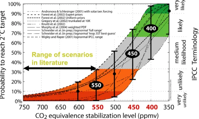
As one of the political actors, the EU has adopted the climate policy goal of limiting the temperature increase to a maximum of 2oC compared to pre-industrial levels (EU, 1996;EU, 2005). New studies have shown that a high degree of certainty in terms of achieving a 2o_C

temperature target is likely to require stabilisation at low GHG concentration (for instance a probability greater than 50% requires stabilisation at least below 450 ppm CO2-eq1). (Figure

1.2.). The stabilisation of GHG concentrations at such a low level will require drastic emission reductions compared to the likely course of emissions in the absence of climate policies. But even for more modest concentration targets such as 650 ppm CO2-eq., emissions

in 2100 will generally need to be reduced by about 50% compared to probable levels in the absence of a climate policy (IPCC, 2001).

Range of scenarios

in literature

Range of scenarios

in literature

Figure 1-2 Relationship between CO2-eq. concentration level and probability of achieving a

2ºC target; the range of current (2005) multigas scenarios in literature is also indicated (Source: Meinshausen, 2006).

1_‘CO

2 equivalence’ expresses the radiative forcing of other anthropogenic radiative forcing agents in terms of

the equivalent CO2 concentration that would result in the same level of forcing. In this paper, the definition of

(23)

A large number of scenario studies have been published that aim to identify mitigation strategies for achieving different levels of GHG emission reductions (see among others Hourcade and Shukla, 2001;Morita and Robinson, 2001). Most of these studies, however, have focused on reducing only the energy-related CO2 emissions, and disregarded options for

the abatement of non-CO2 gases and the use of carbon plantations. Furthermore, the number

of studies looking at stabilisation levels below 550 ppm CO2-eq. is very limited. Thus very

little information exists on mitigation strategies that could stabilise GHG concentrations at the low levels required to achieve a 2-3oC temperature target with a high degree of certainty2.

Given current insights into climate risks and the state of the mitigation literature, there is a very clear and explicit need for comprehensive scenarios that explore different long-term strategies to stabilise GHG emissions at low levels (Morita and Robinson, 2001; Metz and Van Vuuren, 2006).

In this context, the ‘Mitigation Scenarios’ project of the Netherlands Environmental Assessment Agency (MNP)– of which the results are described in this report – took on the task to explore the following three main questions:

1) What would be the required level of emission reductions needed to stabilise emissions at concentration levels 650, 550 and 450 CO2-eq.?

2) What is the potential of various specific options to seriously reduce greenhouse gas emissions (carbon plantations, the use of hydrogen as energy carrier, non-CO2 gases

and renewables)?

3) What portfolios of reduction measures could achieve stabilisation at low-concentrations levels (650, 550 and 450 CO2-eq.) and what could be the costs and

benefits of these portfolios, both at the global and regional level?

The levels 650, 550 and 450 ppm CO2-eq. have been chosen as a range of targets reaching

from medium to low targets.

1.2 General project design and methodology

In 2001, the IMAGE model (Integrated Model to Assess the Global Environment) was used to explore potential developments in the cause-effect chain of climate change under the four storylines of the IPCC-SRES scenarios - all assuming the absence of climate policy (IMAGE-team, 2001). Integrated Assessment models like the IMAGE model and the models associated to IMAGE are also well suited to explore integrated scenarios to stabilise greenhouse gas emissions. In the context of the project ‘’Mitigation Scenarios’ these models were used specifically to explore whether it was possible to identify stabilisation scenarios consistent with limiting global mean temperature increase to only 2-2.5oC.

2_{As a matter of fact, even the number of studies looking at stabilizing at 550 ppm CO}

2-eq. is far lower than for

(24)

The models used are the following:

The IMAGE 2.3 model is an integrated assessment model consisting of a set of linked and integrated models that together describe important elements of the long-term dynamics of global environmental change, such as air pollution, climate change, and land-use change. IMAGE 2.3 uses a simple climate model and a pattern-scaling method based on various GCM model output to project climate change at the grid level. At the grid level, land use change is described by a rule-based system driven by regional demand for, and production of food, timber and fibers. Finally, natural ecosystems are described by an adapted version of the BIOME model.

The global energy model, TIMER 2.0, a part of the IMAGE model, describes primary and secondary demand for, and production of, energy and the related emissions of GHG and regional air pollutants.

The FAIR–SiMCaP 1.1 model is a combination of the multi-gas abatement-cost model of FAIR 2.1 and the pathfinder module of the SiMCaP 1.0 model. The FAIR cost model distributes the difference between baseline and global emission pathways using a least-cost approach involving regional Marginal Abatement Cost (MAC) curves for the different emission sources (Den Elzen and Lucas, 2005).3 MACs for

energy-related sources are derived from the TIMER 2.0 model. The SiMCaP pathfinder module uses an iterative procedure to find multi-gas emission pathways that meet a predefined climate target (Den Elzen and Meinshausen, 2005).

Calculations in all three main models are done for 17 regions4 of the world.

Potentials to

abate GHG

emissions

Baseline

scenarios

Reduction

pathways

MACs

Mitigation

scenarios

Emissions Stabilization objectives Figure 1-3 Overall project scheme.

The project has been set-up in the following steps:

Baseline scenarios. First, the TIMER and IMAGE models are used to determine potential development in the absence of climate policies. This part of the project represents basically an update of the IMAGE implementation of the IPCC-SRES scenarios.

3_{Marginal Abatement Cost (MAC) curves reflect the additional costs of reducing the last unit of CO} 2-eq.

emissions.

4_{Canada, USA, OECD-Europe, Eastern Europe, the former Soviet Union, Oceania and Japan; Central America,}

South America, Northern Africa, Western Africa, Eastern Africa, Southern Africa, Middle East and Turkey, South Asia (incl. India), South-East Asia and East Asia (incl. China) (IMAGE-team, 2001).

(25)

Potential to abate GHG emissions. Second, an assessment was made of the potential and costs to reduce GHG emissions for various emissions sources. In some cases, specific research was performed to update existing information such as for non-CO2

gasses, renewables, hydrogen and carbon plantations.

Development of emission pathways. The FAIR–SiMCaP 1.1 model is used to develop global emission pathways that lead to a stabilisation of the atmospheric GHG

concentration.

Development of mitigation scenarios. The emissions pathways are expressed in terms of specific mitigation action. These are implemented into the TIMER and IMAGE model to evaluate their impacts on the development of the energy system and land use.

Distribution of efforts. The FAIR 2.1 model is used to evaluate the implications of various approaches for regionally allocating the global emission reduction effort and its implications for regional costs and emission trading.

This modeling set-up corresponds to addressing the overall questions raised in section 1.1 and is also partly reflected in the structure of the various papers that are included in this report.

Compared to the previous work (e.g. Van Vuuren et al., 2006) the new scenario analyses presented here have been improved in various ways:

- the set of stabilisation levels has been extended;

- the methodology for defining global emission profiles has been improved; - the set of mitigation options includes more options, like hydrogen use, improved

modeling of carbon sequestration and biomass use combined with carbon removal and storage;

- the analysis includes an extensive uncertainty analyses to test the robustness of results.

All in all, the analyses can be considered as ‘state of the art’ in integrated assessment

modeling of mitigation of greenhouse gases at a global scale. Nevertheless, the analysis also has some limitations to be mentioned. The impacts of climate change have not been assessed, thus also not the cost of inaction. Recent insights into the relationship between global average temperature change and risks from climate change have, however, been explored in another MNP report (MNP, 2005) and by others (see the first section). Moreover, no macro-economic feedbacks of the mitigation costs on economic development pathways have been explored.

1.3 Structure of this report

This report consists of a set of articles rather than a set of chapters. The reason for this is that in addition to their contribution to the overall analysis, each of these chapters was intended to be published separately in scientific journals to be citable in existing scientific literature and the Fourth Assessment Report of the Intergovernmental Panel on Climate Change. The publication of the findings in scientific journals also allows for peer-review of the findings

(26)

presented here. All articles have been submitted to various journals; some have already been accepted. The aim of this report was to bring together the various tranches of analytical work that contributed to the integrated assessment. The report starts with a chapter on the

integrated assessment of low-level stabilisation scenarios, followed by a chapter on the construction of the emission pathways for stabilisation. Next, a number of chapters explore more specific mitigation options. Finally, the aspect of the regional distribution of mitigation costs is addressed.

(27)

2 The role of carbon plantations in mitigating climate

change: potentials and costs

B.J. Strengers, J.G. van Minnen, B. Eickhout

2.1 Introduction

There is mounting evidence that most of the global warming since the mid 20th century is attributable to human activities, in particular to emissions of greenhouse gases (GHGs) from burning fossil fuels and land-use changes (Mitchell et al., 2001). Article 2 of the United Nations Framework Convention on Climate Change (UNFCCC) states its ultimate objective as ‘Stabilisation of greenhouse gas concentrations in the atmosphere at a level that would prevent dangerous anthropogenic interference with the climate system’. A large number of scenario studies have been published that aim to identify mitigation strategies for achieving different stabilisation levels of CO2 (e.g. Morita et al., 2001). However, most of these studies

concentrated on reducing the energy-related CO2 emissions only, leaving aside abatement

options that enhance CO2 uptake by the biosphere. This lack of attention to carbon

sequestration in the scientific literature has been partly compensated since the Kyoto Protocol makes provisions for Annex B countries to partly achieve their reduction commitments by planting new forests or by managing existing forests or agricultural land.

Information made available before the Third Assessment Report (TAR) of the

Intergovernmental Panel on Climate Change (IPCC; Metz et al., 2001) suggested that land has the technical potential to sequester an additional 87 billion tons of carbon by 2050 in global forests alone (Watson et al., 2000). Since the IPCC’s TAR, many studies have

addressed the possibility of carbon sequestration as part of mitigation strategies, although not many integral studies are available. Moreover, differences in terminology and scope make it difficult to compare the different carbon sequestration studies (Richards and Stokes, 2004). Several sectoral studies suggest that land-based mitigation could be cost-effective compared to energy-related mitigation strategies and could provide a large proportion of total mitigation (Sohngen and Mendelsohn, 2003; McCarl and Schneider, 2001).

However, most of these studies work on crude assumptions for future land-use change, a crucial factor determining future land availability for purposes other than carbon plantations (Graveland et al., 2002) or land for modern biofuels (Hoogwijk et al., 2005). For example, Sathaye et al. (in press) based their future projections of carbon sinks on linear extrapolation of continuing deforestation and afforestation rates, whereas Sohngen and Sedjo (in press) only considered an increase in forest product demand, discarding future food demand, which is expected to increase immensely in the coming decades (Bruinsma, 2003).

(28)

This paper presents a new methodology for constructing supply curves and cost-supply curves or Marginal Abatement Curves (MACs) for carbon plantations based on integrated land-use scenarios from the Integrated Model to Assess the Global Environment (IMAGE team, 2001; Strengers et al., 2004). This methodology builds on Van Minnen et al. (2006), which present a method for quantifying the sequestration potential of planting carbon

plantations. This methodology takes land use for food supply into account and obtains a more coherent carbon sequestration potential. Moreover, by basing the MACs on the land-use scenarios of IMAGE 2 and implementing the carbon plantations in IMAGE 2 itself,

overestimation of carbon sequestration potential or unrealistic overruling of the food supply chain is not possible, as in other studies. In these studies, MACs are used directly by

Computable General Equilibrium models and the consequences for other land opportunities are not considered (Criqui et al., in press; Jakeman and Fisher, in press).

Section 2.2 summarises the methodology to determine the carbon sequestration potential and present the methodology for constructing cost supply curves in more detail. Section 2.3 consists of global and regional results to emphasise the regional specificity of our

methodology. Here, we also show the importance of different harvest regimes. Section 2.4 elaborates on the relative importance of different parameters in our methodology via a sensitivity analysis. We draw our presentation of this new methodology to a close with an elaborate discussion that compares our results with those from other studies, and with a number of conclusions.

2.2 Methodology and scenarios

In this approach, the MACs for carbon sequestration potentials are based on geographical explicit simulations in which the availability of potential land can be assessed in different baselines. The carbon potentially sequestered is compared with the natural carbon

sequestered, and the costs of carbon plantations are considered regionally, resulting in supply curves and cost-supply curves for 17 world regions. These curves can be used in an overall framework that compares different CO2 emission mitigation options. We can also estimate

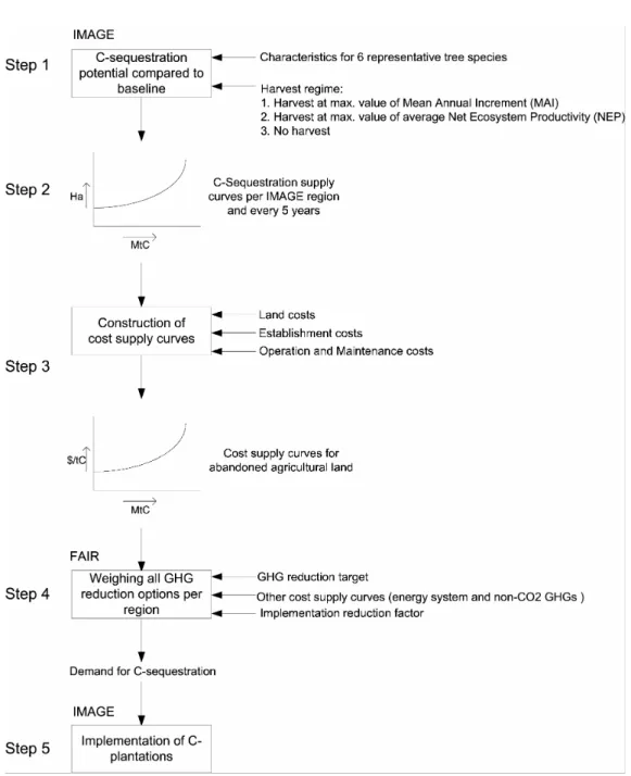
how much carbon sinks can realistically add to an overall mitigation effort aimed at a certain stabilisation level. An overview of the complete methodology is shown in Figure 2.1.

(29)

Step 1: Global C-sequestration potential

In this first step, the carbon sequestration potential of carbon plantations is determined at a grid level of 0.5o longitude x 0.5 o latitude, taking into account the agricultural land needed to meet the food and feed demand. The C-sequestration potential of the best growing trees out of six representative species is quantified by comparing their carbon uptake with the uptake of the natural vegetation that would otherwise grow at the same location. The growth of carbon plantation trees is determined by the Net Primary Production of the natural land cover type that best matches the tree species considered, times an additional growth factor (AGF), which is defined as the additional growth of existing timber plantations compared to the average growth of the natural land cover types. The value attributed to the AGF per tree species is based on an extensive literature review (see Van Minnen et al., 2006). The potential is corrected for the carbon losses due to the conversion. As such, the potential determines the additional aspects when plantations are present compared to the situation in which plantations are absent.

If no harvest takes place, a plantation will grow to a stable level of carbon storage and then provide only little further sequestration over time. If a harvest takes place, we assume that the wood is used to meet the demand for wood. If the harvest exceeds this demand, the remaining wood can then be used to displace fossil fuels. Displacing wood demand and/or fossil fuels can, in theory, last for forever. The displacement of fossil fuels is not modelled explicitly in the current version of the model, but is mimicked by ‘storing’ all remaining useable stems and branches of harvested plantations so that they do not decompose. Leaves, roots and the non-harvested stems and branches enter the soil carbon pools. We assume no leakage (i.e. no changes in fossil fuel demand and/or wood demand). In the default settings we apply a harvest criterion, where the moment of harvesting takes place when the above-ground biomass (AGB) has been maximised. This criterion is common in forestry and reflects the practice of harvesting a forest at the point where the mean annual increment (MAI) decreases. In the IMAGE model this option is mimicked by harvesting when the age of the carbon plantation equals the ‘likely rotation length’.

Since we consider the conversion of natural ecosystems to carbon plantations as being inconsistent with broader sustainability concepts, we allow plantations only on abandoned agricultural land. In this way, the results represent the minimum carbon sequestration potential (see Van Minnen et al., 2006 for more detail on step 1 of this methodology).

(30)

Figure 2-1 Methodology to construct MAC curves for carbon sequestration potential.

Step 2: Supply curves

Based on the carbon sequestration surplus per grid cell, supply curves are constructed for each IMAGE 2 region. The curve for year z is constructed using all grid cells in a region where the average carbon sequestration, corrected for climate change and CO2 fertilisation

effects, is positive in year z. In Figure 2.2, grid cell i covers the yi hectares that potentially

sequester an average of xi MtC in year z. Correction for climate change effects is needed

because the amount of carbon sequestered should be based on stable conditions in terms of climate and since CO2 concentration as also prescribed in the Kyoto Protocol.

(31)

Figure 2-2 A supply curve in year z; grid cell i ( yi Mha) can potentially sequester xi MtC

Because it is not known in advance when a certain potential is actually used in a mitigation effort, and to allow for comparison with other greenhouse gas mitigation options, carbon sequestration is averaged over a predefined period of time. Therefore each point in a supply curve represents the average annual carbon sequestration potential of a grid cell as assigned to a certain time interval [ts,tt]. Ts is the first year the total cumulative carbon sequestration is

positive and tt is the final year of the simulation period. This final year is 2100, or, if no

harvest takes place, the first year in which the annual carbon sequestration decreases below 40% of the overall average value. When there is a harvest, the average carbon sequestration of a plantation between ts and tt equals the average value at the end of the simulation period.

However, when this value at the end of the simulation period is less than 85% of the average value at the end of the last completed harvest cycle, then we assume the average carbon sequestration value at the end of the last completed harvest cycle for the entire plantation period. This situation occurs quite often because in the first years of a harvest cycle the overall average carbon sequestration can temporarily be significantly reduced, since in that period soil respiration often exceeds plant growth, especially for slow-growing species in the high latitudes.

Step 3: Cost-supply curves

The costs of carbon plantations need to be assessed in order to construct MACs out of the supply curves. When dealing with costs, one should keep in mind that vastly different cost estimates of sequestration in forests exist, even among studies that have focused on similar

(32)

regions (especially the United States). In general, the single most important cost factor in producing or conserving carbon sinks is land (Richards and Stokes, 2004). Here, we consider two types of costs: land costs, and establishment costs. Various other types of costs have been evaluated but were not considered further. Operation and maintenance costs, for example, costs for fertilisation, thinning, security and other activities are not considered in most studies on forestry (for review, see Richards and Stokes, 2004). We assume that operation and

maintenance costs are either low (in the case of permanent plantations), or are compensated by revenues from timber or fuel wood (in the case of harvesting at regular time intervals) (Benítez-Ponce, 2005). Likewise, transaction costs and the costs of monitoring or

certification are not considered, since hardly any project experience is currently available (Trines, 2003).

Land costs

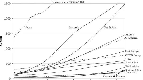
Richards and Stokes (2004) indicate that in a number of studies land costs cover a wide range of estimates. This study uses GTAP data (GTAP, 2004) for land values of agricultural land in 2001 and land costs in GTAP are defined as the sum of value added from crop production and land-based payments such as subsidies (see Table 2.1). The average value of abandoned agricultural land will probably be lower than the average value of existing agricultural land as a result of our assumption that grid cells with the lowest agricultural productivity are

abandoned first. Therefore we may have (slightly) overestimated the land costs in our

analysis. We compared the annual GTAP land values (GTAP, 2004) with capital values from the World Bank (Kunte et al., 1998) (see Table 2.1). These values are defined as the present discounted value of the difference between the world market value of three major agricultural crops (i.e. maize, wheat and rice) from these lands and the crop-specific production costs. The present value of the annual land values from GTAP, computed with the same discount rate as in the World Bank study (i.e. 4%), has turned out to correlate very well for 7 out of 15 regions for which World Bank data exists : USA, South America, northern Africa, southern Africa, OECD Europe, Middle East and Oceania (R2=0.99; although GTAP values are around 1000 US$ higher than World Bank values). No data were was available for Eastern Europe and former Soviet Union): For another five regions (Canada, Western Africa, Eastern Africa, South Asia and Southeast Asia) GTAP values come to around one-third of World Bank results (at R2=0.91). For the remaining three regions (Japan, East Asia and Latin America) GTAP values are considerably higher than the World Bank values. The sensitivity analysis shows the importance of different land costs, which are considerable.

GDP per hectare of ‘useable’ area (see Table 2.1) is an important indicator for estimating how land costs evolve over time. The useable area is defined as the total surface area of a region minus the surface area of hot desert, scrubland, tundra and ice. Adding other factors, such as population density or crop yields does not improve the correlation coefficient (of 0.74). Regional land costs over time (LCR(t)) are calculated as:

(33)

2001 ) ( ) ( Area t GDP C t LC_R = _R× (2.1)

where CR is a regional normalisation factor to make land costs in 2001 equal to the

GTAP-land values (see Table 2.1).

Table 2-1 GDP per ha of ‘useable’ area in 2000 and estimates of land costs based on two different sources: GTAP (GTAP, 2004) and the World Bank (Kunte et al., 1998).

IMAGE 2 Region GTAP 1995US$ ha-1_yr-1 GTAPa 1995US$ ha-1 World Bank 1995US$ha-1 GDP 1995US$ ha-1 CR 1 Canada 87 2130 5224 960 2.8 2 USA 263 6450 6200 10,150 2.6 3 Central America 324 7950 2650 2280 6.8 4 South America 153 3760 2160 860 5.2 5 6 7 8 Northern Africa Western Africa Eastern Africa Southern Africa 152 31 31 45 3720 760 760 1110 2620 1990 2000 500 1840 130 120 310 3.5 2.8 2.8 2.6 9 10 OECD Europe Eastern Europe 423 263 10370 6440 10,080 no data 28,250 3520 2.5 4.4

11 Former USSR 52 1280 no data 280 3.1

12 Middle East 100 2460 1710 2655 2.0 13 South Asia 304 7440 16,515 1410 8.1 14 East Asia 458 11,220 5273 2790 8.7 15 Southeast Asia 289 7085 24,100 1815 6.8 16 Oceania 76 1870 1040 815 2.7 17 Japan 2150 52,720 33,470 150,350 5.6

(34)

Table 2-2 Overview of regional establishment costs. IMAGE 2 Region Establishment costs 1995 US$ ha-1 Source: IPCC, 1996 Establishment costs US$ ha-1

Source: Richards and Stokes, 2004h

1 Canada 456 (343-572)a _300-500

2 USA 473 (160-790)a 140-690

3 Central America 542 (172-890)a,g _387-700

4 South America 395 (290b_-500c₎ 5 6 7 8 Northern Africa Western Africa Eastern Africa Southern Africa No carbon plantations 456 (33-1560)a 343d_(33-1560)a 456 (33-1560)a 9 10 OECD Europe Eastern Europe 352 (296b_-408e₎ 352 (296b_-408e₎ 11 Former USSR 389 (370f_-408e₎

12 Middle East No carbon plantations

13 South Asia 525 (420-630)a _367-550 14 East Asia 500 (50-950)a _46-828 15 Southeast Asia 515c 16 Oceania 395 (290b_-500c₎ 17 Japan 349 (290b_-408e₎ World average 435 400-450

a_{Table 9.29, IPCC (1996);}b_{Temperate afforestation, Table 7.9, IPCC (1996);}c _{Tropical reforestation, Table 7.9, IPCC}

(1996); d_{Lower than African average because of lower per capita GDP;}e_{Temperate reforestation, Table 7.9, IPCC (1996);}f

Boreal reforestation, Table 7.9, IPCC (1996); g_{Table C1, p. 77, Benítez (2005);}h_{US$: here it is not clear to which year}

Richards and Stokes (2004) refer.

Note that the application period of carbon plantations is longer than the period of net

sequestration. Therefore land costs over the complete period need to be assigned to the period in which carbon payments take place. Here, the period before cumulative carbon

sequestration exceeds the sequestration of the natural vegetation, and is called the start-up period (spi). For fast growing tree species, such as eucalyptus and poplar, this period is

usually 0–5 years, whereas for other species it can be 25 years or more. The annual land costs, ALCi(t), are calculated by the following (in 95US$/ha/yr):

(35)

( )

₍

₎

lt s t sp j j sp R i t t t r r r t LC t ALC i i ≤ ≤ ⎟⎟ ⎟ ⎟ ⎟ ⎠ ⎞ ⎜⎜ ⎜ ⎜ ⎜ ⎝ ⎛ + − + ⋅ + × = = ₋ −

∑

− , 1 1 ) 1 ( 1 1 1 (2.2)

where i is the index for a grid cell, r the discount rate (i.e. 4%), and lt the length of the period from ts to tt in years (see also step 2).

Establishment costs

Establishment costs include costs for land clearing, land preparation, plant material, planting and replanting, fences and administrative and technical assistance. Costs of land clearing depend on the original type of vegetation and other (landscape and soil) factors. Estimates on establishment costs as summarised by IPCC (1996) have been translated to the IMAGE 2 regions (Table 2.2). These costs fall well within the range of the initial treatment costs, as reported in Table IX from Richards and Stokes (2004).

Since relatively small variations exist between the regions compared to the ranges within the regions, we decided to use one single average value (435 1995US$/ha), both in time and space. This assumption is supported by the overview study of Sathaye et al. (2001), who state that the cost of planting is relatively uniform and stable in time: here, costs are found from 150 US$/ha to 500 US$/ha.

The establishment costs are translated to annual establishment costs at the grid level as follows:

(

)

(

)

lt s t sp i t t t r r r t AEC i ≤ ≤ + − + ⋅ × = ₋ , 1 1 1 435 ) ( (2.3)

Step 4: Computation of a multi-gas abatement strategy

The MACs developed from carbon sequestration are used as input in the FAIR model (Framework to Assess International Regimes) for differentiation of commitments (see Den Elzen and Lucas, 2003), along with MACs from the energy system and non-CO2 GHGs (Van

Vuuren et al., 2006). The FAIR model was developed to explore and evaluate the environmental and abatement cost implications of various international regimes for differentiating future commitments to meet long-term climate targets. An implementation factor in the FAIR model (see Figure 2.1) mimics the fact that a shortage of planting material, limited availability of nurseries, lack of knowledge and experience, unavailability of credit facilities, land tenure, distrust in governmental policies, and other priorities for the land (e.g. biofuels) may reduce the potential area that can actually be planted. Nilsson and

(36)

Schopfhauser (1995) estimated, for example, that only 275 Mha of carbon plantations will actually be available out of the global total of 1.5 billion ha (=18%). Likewise, in a study on Clean Development Mechanisms (Waterloo et al., 2001), eight implementation criteria are distinguished, including additionality, verifiability, compliance and sustainability. If all eight criteria were to be applied, they estimated that only 8% of the potential area would actually be available. Benítez et al. (2005) indicate that if ‘country risk considerations – associated with political, economic and financial risks’ are included, then carbon sequestration will be reduced by approximately 60%.We use an implementation factor of 1; the consequences of lower values are assessed in Van Vuuren et al. (2006).

Step 5: Implementation of carbon plantations

Finally, the carbon sequestration as demanded by a multi-gas mitigation simulation with FAIR is realised in the IMAGE model by simulating the actual establishment of carbon plantations. Since grid cells can only be converted entirely, the implementation factor

determines the number of the available grids being converted to C-plantations. Logically, the C-sequestration achieved will be checked to see if it is indeed at least equal to the amount required.

Scenarios implemented

We used the four IPCC SRES scenarios (Nakicenovic et al., 2000) to assess the importance of different baselines (Table 2.3). These scenarios (A1b, A2, B1, and B2) explore different possible pathways for greenhouse gas emissions in the absence of climate policy on the basis of two major uncertainties: the degree of globalisation versus regionalisation, and the degree of orientation with respect to economic objectives versus an orientation focusing on social and environmental objectives. New insights have emerged for some parameters: for example, both population scenarios and economic growth scenarios in low-income regions have been lowered (Van Vuuren and O' Neill, 2005). In general, the B2 scenario focuses on possible events under medium assumptions for the most important drivers (i.e. population, economy, technology development and lifestyle). In terms of its quantification, the B2 scenario used here roughly follows the reference scenario of the World Energy Outlook 2004 in the first 30 years. After 2030, economic growth converges to the IPCC B2 trajectory. The long-term UN medium population projection is used for population. The demand for biofuel crops is determined according to Hoogwijk et al. (2005). Trends in the regional management factors for agriculture, which reflect the difference between potential attainable yields and the actual yield level, have been taken from the ‘Adapting Mosaic’ scenario of the Millennium

Ecosystem Assessment (MA, 2005). The assumptions for population, economic growth and management factors in the A1b and B1 scenarios have also been taken from the respective scenarios, ‘Global Orchestration’ and ‘Technogarden’, in the Millennium Ecosystem Assessment. All other assumptions are based on the earlier implementation of the SRES scenarios (Strengers et al., 2004; IMAGE team, 2001).

(37)

Table 2-3 Five indicators in the year 2100 of the IMAGE implementation of four SRES scenarios.

Indicator Unit A1b A2 B1 B2

1 GDP per capita US$ (1995) 75,100 17,690 54,232 36,000

2 Population x billion 6.9 12.6 6.9 9.1

3 CO2 equivalent ppmv 1057 1341 675 928

4 Temp. increase o_C _{3.3 3.7 2.5 3.0}

5 Agricultural land Mha 2004 4512 1859 2671

6 Biofuel crop area Mha 356 237 618 405

7 Potential CP area Mha 938 109 724 790

The differences in socio-economic conditions and environmental conditions (see Table 2.3) have considerable effects on the demands for and growth rate of food, fodder, and biofuel crops and wood, thus on the area needed for agriculture. These different trends result in different areas being potentially available for carbon plantations, both cumulative and over time (Figure 2.3). These areas are used as input for simulating different carbon sequestration potentials. 0 2 4 6 8 10 12 14 16 18 2000 2010 2020 2030 2040 2050 2060 2070 2080 2090 2100 Mha /y A1b A2 B1 B2