Scenarios for exposure of aquatic organisms to plant protection products in the Netherlands : Part 1: Field crops and downward spraying | RIVM

Hele tekst

(1)Scenarios for exposure of aquatic organisms to plant protection products in the Netherlands Part 1: Field crops and downward spraying RIVM report 607407002/2012 A. Tiktak | P.I. Adriaanse | J.J.T.I. Boesten | C. van Griethuysen | M.M.S. ter Horst | J.B.H.J. Linders | A.M.A. van der Linden | J.C. van de Zande. National Institute for Public Health and the Environment P.O. Box 1 | 3720 BA Bilthoven www.rivm.com.

(2) Scenarios for exposure of aquatic organisms to plant protection products in the Netherlands Part 1: Field crops and downward spraying RIVM Report 607407002/2012.

(3) RIVM report 607407002. Colofon. © RIVM 2012 Parts of this publication may be reproduced, provided acknowledgement is given to the 'National Institute for Public Health and the Environment', along with the title and year of publication.. A. Tiktak, PBL Netherlands Environmental Assessment Agency P.I. Adriaanse, Wageningen UR, Alterra J.J.T.I. Boesten, Wageningen UR, Alterra C. van Griethuysen, Ctgb M.M.S. ter Horst, Wageningen UR, Alterra J.B.H.J. Linders, RIVM A.M.A. van der Linden, RIVM J.C. van de Zande, Wageningen UR, Plant Research International Contact: Aaldrik Tiktak PBL Netherlands Environmental Assessment Agency Aaldrik.Tiktak@pbl.nl. This investigation has been performed by order and for the account of the Ministry of Infrastructure and the Environment (research programme M/607407) and the Ministry of Economic Affairs (research programme BO12-007-004), within the framework of Development of risk assessment methodology.. Page 2 of 129.

(4) RIVM report 607407002. Abstract. Scenarios for exposure of aquatic organisms to plant protection products in the Netherlands. Part 1: Field crops and downward spraying In the current Dutch authorisation procedure for calculating the exposure of surface water organisms to plant protection products, drift deposition is considered to be the only source for exposure of surface water organisms. Although drift can still be considered the most important source, atmospheric deposition and drainage may constitute important sources as well. Therefore, RIVM, PBL Netherlands Assessment Agency, Wageningen UR and the Board for the authorisation of plant protection products and biocides have derived a new procedure in which these two potential sources are included. The new procedure, described in this report, is restricted to downward spray applications in field crops. Specific Dutch circumstances The update of the procedure was initiated to bring the Dutch procedure more in line with the EU procedure, which already takes account of drainage. However, typical Dutch adaptations of the procedure remain. In the new procedure, drift is still based on Dutch drift deposition measurements. Characteristic is that the flow velocity of the selected ditch is rather low. Risk management decisions Two boundary conditions were used as starting points for deriving the scenario. First, there was the risk management decision that the scenario should be protective for at least 90 per cent of field ditches. Second, it was assumed that all adjacent fields are treated with the same substance and thus contribute to resulting exposure concentrations in the ditch. Drift reducing measures still important Currently, when spraying plant protection products on fields along surface water, growers should maintain a crop-free buffer zone and use certified sprayers that reduce spray drift deposition by at least 50 per cent. Example calculations with four substances showed that it is worthwhile to invest in further drift reduction. Calculated impacts on water organisms reduced upon applying higher drift reduction when drift was the dominant factor.. Keywords: drainage, DRAINBOW, exposure, PEARL, spray drift, surface water, TOXSWA. Page 3 of 129.

(5) RIVM report 607407002. Page 4 of 129.

(6) RIVM report 607407002. Rapport in het kort. Scenario’s voor blootstelling van waterorganismen aan gewasbeschermingsmiddelen in kavelsloten. Deel 1: Neerwaartse bespuitingen in veldgewassen In de Nederlandse toelatingsbeoordeling voor gewasbeschermingsmiddelen wordt de blootstelling van waterorganismen te eenzijdig berekend. In de huidige beoordeling wordt namelijk alleen rekening gehouden met de mate waarin deze stoffen het oppervlaktewater bereiken via de verwaaide nevel van de gewasbeschermingsmiddelen (drift). Deze nevel ontstaat nadat de middelen over het land zijn gespoten. Hoewel dit de belangrijkste ‘route’ is, blijken twee andere routes ook van belang: via de atmosfeer en via de drainagesystemen in de bodem van de landbouwpercelen. Het RIVM heeft daarom in samenwerking met het Planbureau voor de Leefomgeving, Wageningen UR en het College voor toelating van gewasbeschermingsmiddelen en biociden (Ctgb) deze twee routes aan de blootstellingsscenario’s toegevoegd. Specifiek gaat het hierbij om neerwaartse bespuiting in veldgewassen (akkerbouw, bloembollen en vollegrondsgroenteteelt). Grote hoeveelheid oppervlaktewater in Nederland Deze aanpassing is onderdeel van een herziening van de Nederlandse methode om risico’s van gewasbeschermingsmiddelen te berekenen. Dat is nodig om de methode beter overeen te laten komen met Europese toelatingsprocedures voor dergelijke stoffen, waarin drainage al langer wordt meegenomen. De specifiek Nederlandse omstandigheden zoals de ruime hoeveelheden oppervlaktewater en de eigen driftcijfers blijven gehandhaafd. Kenmerkend voor het nieuwe scenario is dat er sprake is van een lage stroomsnelheid in het Nederlandse slootwater, waardoor stoffen relatief lang in het water blijven. Uitgangspunten Een van de uitgangspunten van het voorstel is de beleidskeuze dat de berekende maximale concentratie van een stof in negentig procent van de sloten onder de norm ligt. In de berekeningsprocedure wordt ook uitgegaan van belasting van het oppervlaktewater door gebruik op alle naastliggende percelen. Driftreducerende maatregelen blijven belangrijk Momenteel zijn telers van veldgewassen verplicht maatregelen door te voeren om de drift langs sloten met minimaal 50 procent te verminderen. Voorbeeldberekeningen met vier stoffen laten zien dat dergelijke driftreducerende technieken belangrijk blijven. In sommige gevallen kunnen aanvullende maatregelen de hoeveelheid drift namelijk nog verder omlaag brengen.. Trefwoorden: blootstelling, drainage, DRAINBOW, drift, oppervlaktewater, PEARL, TOXSWA. Page 5 of 129.


(8) RIVM report 607407002. Preface. A few years ago the Dutch government decided to initiate an improvement of the methodology for the assessment of effects of plant protection products on aquatic organisms. As part of this improvement, the Dutch government established two working groups covering both the effects side and the exposure side of the assessment. This report describes the development and parameterisation of the exposure methodology; the effects side of the assessment is described in Brock et al. (2011). Background reports are published on guidance for the estimation of degradation half-lives in water, the crop-related aspects of crop canopy spray interception, the development of the drainpipe part of the exposure assessment, and the development of the spray drift part of the assessment:  Boesten, J.J.T.I., P.I. Adriaanse, W. Beltman, M.M.S. ter Horst, A. Tiktak, and A.M.A. van der Linden, 2013. Guidance for using available DegT50 values for estimation of degradation rates in Dutch surface water and sediment. Report 284 of WOT unit of Alterra, Alterra, Wageningen.  Van de Zande, J., and M.M.S. ter Horst, 2012. Crop-related aspects of crop canopy spray interception and spray drift from downward directed spray applications in field crops. WUR-PRI report 420, Wageningen, the Netherlands.  Tiktak, A., J.J.T.I. Boesten, R.F.A. Hendriks and A.M.A. van der Linden, 2012b. Leaching of plant protection products to field ditches in the Netherlands. Development of a PEARL drainpipe scenario for arable land. RIVM report 607407003, RIVM, Bilthoven, the Netherlands.  Van de Zande, J.C., H.J. Holterman, and J.F.M. Huijsmans, 2012. Spray drift for the assessment of exposure of aquatic organisms to plant protection products in the Netherlands. Part 1: Field crops and downward spraying. WUR-PRI report 419, Wageningen, the Netherlands. The exposure assessment methodology in this report is restricted to applications with downward spray techniques in field crops. At a later stage, an exposure assessment methodology for applications with upward or sideward spray techniques in fruit crops and tree nurseries will be published. This report is produced within the framework of the working group on exposure of aquatic organisms. The following people have been or are currently members of this working group: Paulien Adriaanse (Alterra), Wim Beltman (Alterra), Jos Boesten (Alterra), Joost Delsman (Deltares), Aleid Dik (Adviesbureau Aleid Dik), Corine van Griethuysen (Ctgb), Mechteld ter Horst (Alterra), Janneke Klein (Deltares), Ton van der Linden (RIVM), Jan Linders (RIVM), Aaldrik Tiktak (PBL) and Jan van de Zande (PRI). The authors of this report thank the members of this working group for their opinions and suggestions for improvement.. Page 7 of 129.


(10) RIVM report 607407002. Contents Summary—11 1 1.1 1.2 1.3 . Introduction—13 Background—13 Remit—14 Structure of report—14 . 2 2.1 2.2 2.3 . Outline of scenario development procedures—15 Endpoint of the exposure assessment—15 Position in the tiered assessment scheme—19 Procedure for developing the exposure scenario—20 . 3 3.1 3.2 3.3 . Databases for scenario selection—23 Soil data—23 Dimensions of water courses—24 Spray drift—26 . 4 4.1 4.2 4.3 4.4 4.5 . Selection of the spray drift scenario—29 Approach—29 Impact of wind speed, wind angle and ditch dimensions—30 Selection of the scenario for downward spraying—32 Multiple applications—35 Conclusions—37 . 5 5.1 5.2 5.3 5.4 5.5 5.6 5.7 . Selection of the drainpipe scenario—39 Approach—39 Application of PEARL to the Andelst dataset—40 Parameterisation of the drainpipe scenario—41 Calculation of the overall 90th percentile with GeoPEARL—42 Selection of the target temporal percentile—44 Temporal percentile to be used in the exposure assessment—48 Conclusions—50 . 6 6.1 6.2 6.3 6.4 . TOXSWA parameterisation of scenarios—51 Conceptual model—51 Suspended solids and sediment components—52 Temperature—56 Hydraulic characteristics of selected ditches—56 . 7 7.1 7.2 7.3 7.4 . Parameterisation of other scenario properties—63 Spray drift parameterisation—63 Interception—67 Atmospheric deposition—69 PEARL parameterisation—71 . 8 8.1 8.2 8.3 . Drift-reduction measures—73 Drift-reduction technology – current rules and regulations—73 A matrix approach for drift-reducing measures—75 Spray drift deposition on surface water – an example—76 . Page 9 of 129.

(11) RIVM report 607407002. 9 9.1 9.2 9.3 . User-defined input—79 Overview of DRAINBOW user interface—79 Crop type, application schedule and drift mitigation options—80 Substance properties—81 . 10 10.1 10.2 10.3 10.4 10.5 10.6 10.7 . Examples—85 Substance IN in lilies—85 Substance IP in lilies—89 Substance FP in potatoes—92 Substance HT in potatoes—95 Effect of assumptions on treatment of upstream catchment—98 Sensitivity of the exposure concentration to DegT50 in water—101 Conclusions—101 . 11 . Proposal for a tiered assessment scheme—105 . 12 12.1 12.2 12.3 12.4 12.5 12.6 . Discussion and conclusions—109 Scenario development—109 Spray drift—110 Drainage—111 Exposure in the ditch—112 Example calculations—113 Development of other tiers—113 . 13 . Main recommendations—115 List of abbreviations—117. References—119. Appendix 1 Properties of the example substances—125. Appendix 2 Model versions used in this study—129 . Page 10 of 129.

(12) RIVM report 607407002. Summary As part of the proposed revised assessment procedure for exposure of aquatic organisms to plant protection products in the Netherlands, an exposure scenario was developed for downward spraying in field crops. This scenario corresponds to the 90th spatio-temporal percentile of the annual maximum concentration in all ditches that receive input from spray drift and drainpipes. The scenario is intended to be a second-tier approach, to be preceded by a first tier consisting of one or more of the FOCUS surface water scenarios and succeeded by higher tiers considering refinements such as better input parameters and drift reduction measures. To the best of our knowledge the surface water scenario presented in this report is the first regulatory scenario that has been derived systematically using probabilistic and geostatistical modelling based on the requirement of a specified spatio-temporal percentile of a concentration distribution (in this case the 90th spatio-temporal percentile of the population of annual peak concentrations in ditches that are at the border and downwind of treated fields and that receive drain water from these treated fields). The endpoint of the exposure assessment is a spatio-temporal percentile of the annual maximum concentration in all relevant arable field ditches. The spray drift model IDEFICS and a macropore version of the leaching model GeoPEARL were used to simulate the exposure concentration for the entire population of ditches. This resulted in the selection of a 90th percentile scenario. For this scenario, a non-stationary flow version of TOXSWA was parameterised. Most ditch parameters could be derived from national databases. Where information from national databases was not available, parameter values were taken from FOCUS (2001). The selected ditch is a water course typical of river clay areas and has a lineic volume of 0.55 m-3 m-1 and a water depth at the wet winter situation of 0.23 m. TOXSWA simulations showed that most of the time, the water moves slowly (< 1.5 cm d-1), so the residence time of substances in the ditch can be high. For the spray drift part of the exposure assessment, new spray drift deposition curves were developed. These curves describe the relation between the distances from the edge of the field and spray drift deposition. The spray drift curve to be used in the exposure assessment depends on crop type, crop development stage and treatment type. A decision tree was built to facilitate the selection of the appropriate curve. Spray drift deposition is calculated using a fixed water depth of 0.1905 m. This is the water depth for a situation where the discharge from the ditch is equal to the base flow. The drift deposition calculated with the new spray drift curves is higher than the spray drift deposition data that is currently used in the Dutch authorisation procedure. The drainpipe scenario was based on data from a field experiment in a cracking clay soil. Additional data was used to extend this dataset to a 15-year period, so that the exposure assessment could be carried out for a multi-year period (in accordance with FOCUS 2001). This was considered necessary to reduce the effect of time of application of the plant protection product on the predicted exposure concentration. A sensitivity analysis showed that this strategy worked well for most substances. Only in the case of a quickly degrading, very mobile substance did the predicted exposure concentration vary by 50 per cent when the application date was shifted a few days. Page 11 of 129.

(13) RIVM report 607407002. So the exposure assessment results in a frequency distribution consisting of 15 annual peak concentrations. An analysis showed that the 63rd percentile of this frequency distribution corresponded well with the overall 90th percentile simulated with GeoPEARL (the target concentration). The target concentration increased with increasing DegT50 and decreased with increasing Kom. The predicted differences of the target maximum concentration were small compared with differences of the leaching concentration as predicted by the convectiondispersion equation (Boesten and Van der Linden 1991). This was judged plausible, because the maximum concentration is primarily caused by preferential flow where the substance bypasses most of the reactive part of the soil profile. Example calculations carried out for four substances show that the contribution of spray drift to the maximum annual concentration ranged from 40 to 100 per cent when using a sprayer in the minimum required spray drift reduction class of 50 per cent. Spray drift reduction is therefore still an efficient tool in reducing the exposure of aquatic organisms. However, when spray drift is reduced to a drift reduction class of 95 per cent, atmospheric deposition or drainage becomes the dominant source for half of the considered substances. The low flow velocity in the ditch in combination with low dissipation rates of substances in water caused the concentration of three example substances to build up in the water-sediment layer over the years. As a result, the exposure concentration was above zero during the entire 15-year evaluation period. For two of the example substances, the difference between the maximum concentration averaged over 21 days and the maximum peak concentration was small. This implies that the difference between acute and chronic exposure concentrations is small. As described earlier, the 63rd percentile of the maximum annual concentration was selected from a time series of 15 years. The simulations showed that the year corresponding to the 63rd percentile differed between the four substances. In some cases, selecting another drift-reducing technology or another timeaveraging window caused another year to be selected as well.. Page 12 of 129.

(14) RIVM report 607407002. 1. Introduction. 1.1. Background The risk assessment of plant protection products (PPP) has a long history in the Netherlands. Environmental risk assessment was explicitly introduced in Dutch law in 1962 (Pesticide Act 1962) and has since then been substantiated and defined in more quantitative terms. The Pesticide Act of 1962 was repealed in 2007 and replaced by the Plant Protection Products and Biocides Act of 17-02-2007, which contains articles on environmental risk assessment equivalent to the latest version of the Pesticide Act of 1962. Risk assessment for aquatic organisms has been part of the authorisation procedure of plant protection products, since 1995 explicitly laid down in a quantitative way in the Decree Environmental Criteria Pesticides, succeeded by the Regulation on Plant Protection Products and Biocides of 26 September 2007. In the Regulation, it is stated that the assessment of the risk for aquatic organisms is according to national specific methodology. The exposure of aquatic organisms is calculated using the TOXSWA model (Adriaanse 1996, Ctgb 2010), taking into account drift as the only source of the plant protection product. Also for drift emissions, national specific drift percentages are taken (Ctgb 2010). In evaluation procedures at European level, risk assessment for aquatic organisms is slightly different from the procedure in the Netherlands (EU 1991, 2009). Exposure assessment is performed using the TOXSWA model, but with a different version (FOCUS 2001). The main deviations are slightly different dimensions of the edge-of-field water course, different drift emission percentages and the inclusion of runoff and drainage as potential sources of plant protection products. In 2000 the Water Framework Directive (WFD) was established and put into force (EU 2000). The aim of the WFD is to protect all water bodies and establish good chemical and good ecological quality of the water bodies. The WFD forces national authorities to set standards for water quality which, in contrast to earlier legislation in the Netherlands, have legal liability. This means that responsible authorities have to take measures in order to reach the quality standards if the standards are not met. Measures might include the withdrawal of or change in the authorisation of a plant protection product. In this sense, there is feedback of monitoring results to the authorisation procedure. The Dutch government considered the current Dutch authorisation procedure as no longer defensible in view of the procedures at European level. Furthermore, questions were raised on the compatibility of the authorisation procedure and the requirements as described in the WFD. For these reasons, the Dutch government decided to initiate an improvement of the methodology for the assessment of the effects of plant protection products on aquatic organisms. In order to establish a comprehensive methodology, the Dutch government initiated six working groups to cover various aspects of the new methodology, including a working group on the exposure of aquatic organisms. The remit of the working group on exposure is given in the following section.. Page 13 of 129.

(15) RIVM report 607407002. 1.2. Remit As pointed out in the previous section, the Dutch government decided to initiate an improvement of the methodology for the assessment of the effects of plant protection products on aquatic organisms. A working group was established to develop new procedures for exposure assessment in edge-of-field ditches (in line with EU-Regulation 1107/2009). The following boundary conditions were set with respect to the procedures:  They should be scientifically based and defensible and follow the generally accepted principles of risk assessment as laid down in EU-Regulation 1107/2009.  They should allow for tiered approaches.  They should take into account realistic worst case conditions (realistic worst case being more exactly defined as the 90th percentile of the exposure concentration).  They should deliver various types of concentration for the realistic worst case, the types of concentration being defined by the working group on ecotoxicological effects (in other words: exposure and effect assessment should be adequately linked).. 1.3. Structure of report The remit of the working group states that procedures have to be developed for edge-of-field water courses. The domain of the current scenario is limited to field crops and downward spraying techniques (see Section 2.1). All other scenarios will be reported on later. The report starts with a description of the endpoint of the exposure assessment and general procedures (Chapter 2). Then a description is given of the databases used for scenario development (Chapter 3). Chapters 4 and 5 describe the selection of the spray drift scenario and the development of the drainpipe scenario, respectively. Simplified models for the behaviour of substances in water courses were used in order to obtain peak concentrations of a substance in surface water. More detailed descriptions of the scenario selection are given in Tiktak et al. (2012b) and Van de Zande et al. (2012). Chapter 6 summarises the parameterisation of ditch properties, and other fixed scenario properties are given in Chapter 7. Chapter 8 describes the drift-reducing measures that can be introduced. Chapter 9 describes the user-defined model inputs. Example calculations are provided in Chapter 10. The scenarios are proposed to be part of a tiered assessment scheme (Chapter 11). Finally, Chapter 12 gives conclusions and recommendations for further investigation and the implementation of the methodologies.. Page 14 of 129.

(16) RIVM report 607407002. 2. Outline of scenario development procedures. This chapter gives an overview of the general procedures that were used to select and parameterise the edge-of-field scenario. First, the endpoint of the exposure assessment is discussed (Section 2.1). The edge-of-field scenario is intended to be a second-tier scenario. Section 2.2 describes the general set-up of tiered assessment schemes; a proposal for a tiered assessment scheme for the exposure of aquatic organisms is presented in Chapter 11. Section 2.3 gives an overview of the scenario development. In contrast to earlier procedures (FOCUS 2001), the current scenario has been derived systematically using probabilistic and geostatistical modelling based on the requirement of a specified spatio-temporal percentile of a concentration distribution (in this case the 90th spatio-temporal percentile of the population of annual peak concentrations in ditches that are at the border and downwind of treated fields and that receive drain water from these treated fields).. 2.1. Endpoint of the exposure assessment. 2.1.1. Risk management decisions In line with FOCUS (2000), the responsible Dutch ministries decided that the endpoint of the exposure assessment of aquatic organisms should be the 90th percentile of the concentration in Dutch ditches (see Section 1.2). The ministries also decided that the population of ditches to which this percentile applies should be limited to those ditches that will potentially receive both a spray drift load and a drainpipe load of a plant protection product. Figure 1 gives a schematic representation of this population of ditches. The representation shows that this population may be a small subpopulation of the total population of ditches in the Netherlands. An authorisation is usually requested for use in a specific crop or crop category. The ministries decided that the crop should be the entry for the exposure assessment. If an authorisation is requested for a crop category, an assessment for all crops within this category must be done and the maximum concentration of these assessments should be used. The ministries further decided that only one scenario should be developed for field crops in the Netherlands, so the 90th percentile applies to the total area of field crops. An authorisation is, however, usually requested for a specific crop or crop category. The 90th percentile of the concentration can be higher or lower for a specific crop or crop category. The ministries accepted therefore that this scenario may be too conservative for part of these crops or crop categories and not conservative enough for the other part of these crops. In the Netherlands, ditches are classified into three groups (see Section 3.2), i.e. small or temporarily dry ditches (‘tertiary ditches’), ditches narrower than 3 m (‘secondary ditches’) and ditches wider than 3 m at water level (‘primary ditches’). All these ditch types may be edge-of-field ditches. The ministries decided that all these ditch types – including temporarily dry ditches – should be included in the population of ditches. Larger water bodies (ponds, lakes and rivers) were not included in the population, because they are usually not edgeof-field water courses. Page 15 of 129.

(17) RIVM report 607407002. Figure 1 Schematic representation of the population of Dutch ditches (lines in the diagram) to be considered in the estimation of the percentile of the concentration of PPP in the surface water 2.1.2. Operational decisions The spray drift part of the exposure assessment depends strongly on the application technique (downward versus upward and sideward spraying). As will be described in detail in Chapter 4, the spray drift estimates in the scenario calculations will be based on averages of measurements for a certain application technique. It will be ensured that these estimates result in a 90th percentile predicted environmental concentration (PEC) by selecting a certain ditch. The estimates of leaching from drainpipes will be based on a certain soil scenario (Andelst; see Chapter 5 for details). The exposure assessment methodology in this report is restricted to applications with downward spraying techniques in field crops. At a later stage, an exposure assessment methodology for applications with upward or sideward spraying techniques in fruit crops and tree nurseries will be developed. However, as will be described in Chapter 7, it may also happen in Dutch agriculture that plant protection products are applied with upward or sideward spraying in field crops (e.g. in hop) or with downward spraying in fruit trees (herbicides). Table 1 shows all possible options for the ditch and soil scenarios for these two crop categories plus for the crop category ‘permanent grassland’ (this last group was added to give a complete overview of Dutch agricultural crops). For permanent grassland, the responsible Dutch ministries have not yet decided whether this should be based only on drained grassland (as was done for the field crops; see previous section). So the exposure assessment in this report addresses only one of the six combinations of crop categories and application technique (downward spraying in field crops) in Table 1. However, this combination is expected to include the majority of applications of plant protection products in agriculture in the Netherlands. Page 16 of 129.

(18) RIVM report 607407002. Table 1 Overview of edge-of field scenarios for exposure of aquatic organisms. This report is limited to downward spraying in field crops (upper-left cell of table). Soil scenario Ditch scenario Crop Applications with downward spraying. Applications with upward/sideward spraying. Field crops. Ditch 601001 (Figure 14) based on downward spray drift measurements and all drained arable land (this report). Ditch based on upward/sideward spray drift measurements and all drained arable land (to be defined later). Andelst (this report). Fruit crops and tree nurseries. To be developed later based on downward spray drift measurements from 2011 and all drained arable land. Ditch based on upward/sideward spray drift measurements and all drained arable land (to be defined later). Probably Andelst (to be decided later). Permanent grassland. To be developed later based on downward spray drift measurements and all drained and/or undrained grassland (political choice still to be made).. Not relevant. To be developed later. As mentioned above, our exposure assessment methodology is restricted to downward spray applications in field crops. EFSA (2004) described approaches for aquatic exposure assessment methodologies for non-spray applications including granules and seed treatments. EFSA (2004) showed that dust deposition resulting from such non-spray applications may be significant and should therefore be included in the exposure assessment. Therefore we recommend developing also aquatic exposure assessment methodologies for non-spray applications based on the recommendations of EFSA (2004). An important step in linking exposure and effect assessment is the identification of the ecotoxicology relevant concentration (ERC). Brock et al. (2011) proposed that the endpoint of the exposure assessment should be the annual peak concentration or the annual maximum time-weighted average (TWA) value within a calendar year. Due to the non-linearity of the relation between soil and PPP parameters on the one hand and predicted environmental concentrations on the other, the result of the selection of a 90th percentile scenario may be different for different ecotoxicologically relevant concentrations. Using the peak concentration for the scenario selection may result in a different scenario from Page 17 of 129.

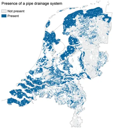
(19) RIVM report 607407002. that obtained using a time-weighted average concentration. Taking also the sediment into consideration may again lead to a different scenario. Based on guidance provided by the ELINK workshop (Brock et al. 2009), the working group decided to base the selection on the annual peak concentration in the surface water. The ELINK workshop stated that an effect assessment based on acute toxicity data should always be compared with the peak concentration, whilst in chronic risk assessments in first instance also the peak concentration and under certain conditions a time-weighted average concentration may be used. Given the time constraints, the working group decided not to develop scenarios for the exposure of organisms in the sediment. An important aspect of the risk assessment applies to the statistical population of exposure concentrations for which the scenario is intended (EFSA 2012). The statistical population has both a spatial and a temporal aspect. With respect to the spatial aspect, the working group decided that the population of ditches should be limited to ditches adjacent to arable land. Figure 2 shows that a large proportion of Dutch arable land (40 per cent) is pipe-drained. We excluded ditches in grassland areas from the population of ditches, because the use of plant protection products in grassland is small compared with use in arable land.. Figure 2 Presence of a pipe drainage system in the Netherlands (Kroon et al. 2001). The 90th percentile of the exposure concentration applies to ditches in the blue area. As described before, the ERC is a peak or TWA concentration. The peak concentration differs between years. The working group therefore decided that the temporal statistical population of concentration should include multiple years. By simulating multiple years, the influence of application time on the simulated peak concentration is also reduced. Brock et al. (2011) proposed that all peak concentrations within a calendar year should be used, so they applied Page 18 of 129.

(20) RIVM report 607407002. no time window in the scenario selection procedure. The working group decided that all annual peak concentrations should be used independently, which implies that there is no distinction between space and time. The working group decided that 100 m of ditch should be used for the evaluation, which is in line with FOCUS (2001). Within a ditch, the substance concentration is variable due to the variability of spray drift deposition. Nevertheless, the working group proposes to use the average substance concentration across the 100 m evaluation ditch. This is a neutral choice: for fish a larger averaging length would have been better and for non-moving organisms a smaller averaging length would have been better (T.C.M. Brock personal communication 2010). In the case of crop rotations, the working group proposes to base the exposure assessment on the cropping year that generates the highest concentration (see Chapter 11 for details). Let us consider as an example an exposure assessment for applications of a substance in two cropping years. In such a case two scenario calculations have to be carried out (one for the first cropping year and one for the second cropping year) and the highest PEC of the two calculations has to be selected.. 2.2. Position in the tiered assessment scheme As described by EFSA (2010a), tiered approaches are the basis of environmental risk-assessment schemes that support the registration of plant protection products. EFSA (2010a) defines a tier as a complete exposure or effect assessment resulting in an appropriate endpoint (in this case the PECSW). The rationale of tiered approaches is to start with a simple conservative assessment and to carry out additional, more complex work only if necessary (so implying a cost-effective procedure for both notifiers and regulatory agencies). The general principles of tiered exposure approaches are (EFSA 2010a):  Lower tiers are more conservative than higher tiers.  Higher tiers are more realistic than lower tiers.  Lower tiers usually require less effort than higher tiers.  In each tier all available relevant scientific information is used.  All tiers aim to assess the same exposure goal. In short, the tiered exposure assessment needs to be internally consistent and cost-effective and to address the problem with increasing accuracy and precision when going from lower to higher tiers. These principles permit moving directly to higher tiers without performing the assessments for all lower tiers (EFSA 2010a). The definition of a tier by EFSA (2010a) implies that decision flow charts for e.g. estimating model input parameters such as the DegT50 in water do not contain tiers because these flow charts do not consider a complete exposure assessment resulting in an appropriate endpoint. Therefore we will call such flow charts ‘stepped approaches’. The scenario for downward spraying and field crops described in this report is intended to be a second-tier approach, to be preceded by a first tier consisting of one or more of the FOCUS surface water scenarios. Higher tiers will consider refinements such as better input parameters, emission reduction measures for Page 19 of 129.

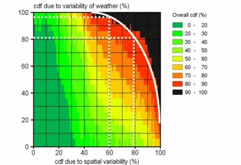
(21) RIVM report 607407002. spray drift, and scenarios that are better targeted to the risk assessment case considered (see Chapter 11).. 2.3. Procedure for developing the exposure scenario The endpoint of the exposure assessment is the 90th percentile of the annual maximum concentration in all ditches that potentially receive plant protection products from spray drift and drainpipes (Figure 1). Crops are usually not sprayed during large rainfall (and drainage) events, so we assumed that the peak concentration is caused by either spray drift or drainage. The advantage of this assumption is that the spray drift and drainpipe scenarios could be developed independently of each other. The peak concentration resulting from drainage is less sensitive to ditch dimensions than the peak concentration resulting from spray drift. The main reason is that a small volume of drainage water completely refreshes the water initially present in most edge-of-field ditches (Tiktak et al. 2012b). The development of the exposure scenario was therefore structured as follows: (i) selection of a ditch that ranks at the 90th percentile in the cumulative distribution of peak concentrations in surface water resulting from drift input, (ii) selection of the drainpipe scenario, and (iii) parameterisation of the ditch using information from the first two steps. The three steps are further explained below.. 2.3.1. Selection of a ditch based on spray drift input The endpoint of the exposure assessment is a percentile, which can only be determined if the peak concentration is known for the entire population of ditches and for the entire range of possible weather conditions. The spray drift model IDEFICS (Holterman et al.1997) was used to simulate the peak concentration in 66 ditch types and 700 combinations of wind direction and wind speed, resulting in 46,200 possible peak concentrations. These 46,200 peak concentrations together represent the entire population of possible ditches and weather conditions, so that it was possible to derive a cumulative frequency distribution function from which the 90th percentile concentration resulting from spray drift could be derived. The 90th percentile concentration can occur at different combinations of ditch type and weather conditions, as can be seen from the contour diagram in Figure 3. For instance, the points X=80 per cent, Y=80 per cent and X=60 per cent, Y=97 per cent both yield an overall 90th percentile of the peak concentration. Further selection criteria were therefore necessary. Application of these additional criteria resulted in the selection of one ditch. More details on the development of the spray drift scenario are given in Chapter 4.. Page 20 of 129.

(22) RIVM report 607407002. Figure 3 Example contour diagram of the overall percentiles of the peak concentration in ditch water. The X-coordinate corresponds with the percentile of the cumulative spatial distribution and the Y-coordinate with the cumulative distribution due to variability of weather conditions. The solid white line corresponds with the 90th overall concentration. The dashed white lines refer to the example combinations described in the text. The IDEFICS (version 3.4) simulations were done for a standard situation with a 50 per cent drift-reducing nozzle and with the last nozzle position at 1.375 m from the top of the ditch bank. The 50 per cent drift-reducing nozzle was adopted because this is the minimum requirement for drift-reducing techniques at the moment. We assumed that the selected scenario would also be representative for the 90th percentile concentration if another (e.g. 90 per cent) drift-reducing nozzle had been used. This assumption allows the use of multiple drift-reducing packages in combination with the selected ditch (see Section 7.1 for details). 2.3.2. Selection of the drainpipe scenario The drainpipe scenario was based on data from the Andelst experimental field site (Scorza Júnior et al. 2004), because at this field site sufficient data was available to parameterise the pesticide fate model PEARL. The advantage of taking a real site was that full benefit could be taken of the experimental data, so that a consistent and credible drainpipe scenario could be built. Drainpipe input is calculated with a new version of the pesticide fate model PEARL (Tiktak et al. 2012a, 2012c). A new version of PEARL was necessary, because the version that is currently used in authorisation procedures (Leistra et al. 2001) does not include a description of preferential flow through macropores. Preferential flow is considered to be the key driver for the peak concentration in drain water. The Andelst dataset covers a period of approximately one year, so we extended the dataset to a 15-year period using data from nearby monitoring stations. Long-term simulations considerably reduce the effect of application time on drainpipe input. By linking the drainpipe scenario with the ditch selected in the Page 21 of 129.

(23) RIVM report 607407002. previous section, 15 annual peak concentrations in ditch water could be calculated. The target for the drainpipe assessment should be the 90th percentile of the peak concentration in ditches adjacent to fields growing field crops that potentially receive input from drainpipes. The overall distribution of the peak concentration is simulated with a spatially distributed version of PEARL that is linked to a metamodel of TOXSWA (Tiktak et al. 2012b). Analogous to the distribution of the peak concentration resulting from spray drift, the overall frequency distribution function of the peak concentration resulting from drainpipe input has a spatial component and a temporal component. The spatial component results in this case from e.g. the distribution of soils and ditches, whereas the temporal component results from variability in the weather between the years. By selecting the Andelst field site, we fixed the spatial percentile, and indirectly also the temporal percentile. This can be seen in the same contour diagram as discussed before (Figure 3): if the X-coordinate is fixed, then only one Y-coordinate corresponds to the overall 90th percentile. For instance, if the spatial percentile is 60 per cent, then the temporal percentile should be 97 per cent. The relative ranking of locations with respect to the concentration in drain water is substance dependent; hence also the spatial percentile of the Andelst site is substance dependent. Because the spatial percentile is directly linked to the temporal percentile, the target temporal percentile is also substance dependent. Further details on the drainpipe scenario and the derivation of the target temporal percentiles are given in Chapter 5. 2.3.3. Parameterisation of the ditch The fate of the substance in ditch water is calculated with version 3.2.4 of the TOXSWA model. In this new version a simplified version of a non-stationary flow solution, i.e. simple ditch scenario concept (Opheusden et al. 2011), was recently implemented. The ditch receives input from base flow and drainage simulated with PEARL, and TOXSWA simulates the water depth and the corresponding ditch volume. Section 4.3 describes how a ditch was selected. TOXSWA was parameterised in such a way that most of the time the water level was close to the water level of the selected ditches. This was done by calibration of the height of the weir crest and the distance from the end of the ditch to the weir. Maintaining the water level close to the water level of the selected ditches ensures that the initial concentration in ditch water is consistent with the 90th percentile concentration in all ditches. More details on the TOXSWA parameterisation are given in Chapter 6.. Page 22 of 129.

(24) RIVM report 607407002. 3. Databases for scenario selection. The endpoint of the exposure assessment is the 90th overall percentile of the peak concentrations in ditches that potentially receive input from spray drift and drainpipes. This percentile is derived from the frequency distribution function of the peak concentration for the entire population of ditches and for the entire range of possible weather conditions. Two models were used, i.e. IDEFICS (Holterman et al. 1997) for spray drift deposition and a macropore version of GeoPEARL (Tiktak et al. 2002, 2012c) for drainpipe input. Most parameters for these two models were derived from national databases. These databases are briefly described in this chapter.. 3.1. Soil data A new version of GeoPEARL was developed, which contains a description of preferential flow through macropores (Chapter 5). All macropore parameters were related to data in a database that was originally developed for the spatially distributed nutrient emission model STONE (Kroon et al. 2001, Wolf et al. 2003). Clay content is a crucial soil parameter for the macropore version of PEARL. In the Netherlands, drained soils can be roughly subdivided into two groups based on clay content, i.e. rigid, non-shrinking, sandy soils with a clay content of less than 8 per cent and shrinking, clay soils with a clay content of over 8 per cent (Figure 4). The clay soils can further be divided into fluvial clays in the centre of the country and maritime clays in the coastal regions. The highest clay contents (> 50 per cent clay) are found in the fluvial deposits. Organic matter content is another important parameter in pesticide fate models. The lowest values of the organic matter content are found in marine clay soils and slightly higher values are found in fluvial deposits (Figure 4). The organic matter content used within GeoPEARL is the nominal (i.e. most frequently occurring) value within map-units. It is known, however, that organic matter is related to land-use type (De Vries 1999). This causes a systematic bias of the organic matter content for arable soils. How this systematic bias is dealt with, is described in Section 5.5. The Mean Lowest Groundwater (MLG) level is an important parameter, because macropores are generally limited to this depth (Chapter 5). The MLG level is generally shallow (80–100 cm) in the riverine region and deep in the coastal clay region. Drain depth follows roughly the same spatial pattern, the deepest drains occurring in recently reclaimed polders.. Page 23 of 129.

(25) RIVM report 607407002. Figure 4 Basic data for the GeoPEARL model. MLG refers to the Mean Lowest Groundwater level. Only drained soils are shown, because the population of interest is limited to these soils (Section 2.1).. 3.2. Dimensions of water courses To calculate the concentration of the substance in the water, the models need information about ditch dimensions, such as the width of the water surface and the water depth (Figure 5). Some information about the width of the water courses can be found on the digital topographical map of the Netherlands (TOP10 vector). This information is too generic for our purpose, however, because water courses are shown in three broad categories only, i.e. small or temporarily dry water courses (‘tertiary ditches’), water courses that have a width of less than 3 m (‘secondary ditches’), water courses that have a width of 3–6 m (‘primary water courses’) and water courses that have a width of 6-12 m. Page 24 of 129.

(26) RIVM report 607407002. Figure 5 Characteristics of water courses described in Massop et al. (2006) A more detailed description of ditch characteristics was obtained from Massop et al. (2006). Based on field inventories, they showed that there is a good correspondence between the geohydrological characteristics of the subsoil and ditch characteristics. Geohydrological characteristics are available for 22 socalled hydrotypes. For each combination of hydrotype and for three ditch classes shown on the digital topographical map, they calculated median values and standard deviations of the ditch characteristics, as shown in Figure 5. The ensemble of all median ditch properties is called a standard ditch profile, so the total number of standard ditch profiles was 66. Maps of both hydrotypes and ditch classes are available, so that it was possible to establish the spatial distribution of the ditch profiles. The spatial distribution of two important ditch characteristics, i.e. the water depth and the water volume per unit ditch length (the lineic volume) is shown in Figure 6. The spatial pattern is plausible with high water volumes in the clay region and low water volumes in the sand region.. Page 25 of 129.

(27) RIVM report 607407002. Figure 6 Median water depth in water courses (upper panel) and lineic water volume (lower panel). Figures are shown for secondary and tertiary water courses as shown on the Dutch digital topographical map. Values are for a socalled ‘wet winter period’. Note the different legends.. 3.3. Spray drift The spray drift database is based on field measurements of spray drift that were performed between 1988 and 2005 (Van de Zande et al. 2012). The aim of the measurements was to determine the effect of drift-reduction technologies (DRT) compared with generally used application techniques (referred to as the reference spray technique). This was done for three crop categories, (i) field crops including bare soil surface, (ii) fruit crops (apples) in the full leaf situation and in the dormant situation, and (iii) nursery trees of different sizes. For each of these three categories, a reference spray technique and several driftreduction techniques were defined. For each crop category, several driftreduction technologies are available; these technologies were generalised into four classes of spray drift reduction, i.e. 50 per cent, 75 per cent, 90 per cent and 95 per cent drift reduction (see also Section 8.1). Page 26 of 129.

(28) RIVM report 607407002. Drift measurements All drift measurements were carried out according to the ISO standard 22866 (ISO 2006) adapted for the situation in the Netherlands (CIW 2003). Spray drift deposition was measured on ground surface at the downwind edge of an experimental field with a crop. The measurements were done regularly during the growing season to obtain an ‘average crop season’ with respect to crop height and canopy density. Spray drift measurements were carried out by adding the fluorescent dye Brilliant Sulfo Flavine (BSF; 3.0 g L-1) and a surfactant (Agral; 0.1 per cent) to the spray agent. All drift measurements were carried out in at least eight replicates. Reference spray technique for downward directed spraying The reference spray technique in field crop spraying is the use of a boom sprayer, applying 300 L ha-1 using TeeJet XR11004 spray nozzles (3 bar spray pressure, medium spray quality; Southcombe et al. 1997) with a boom height of 50 cm. The sprayed swath width is 24 m. For arable crop spraying with boom sprayers, 124 measurements are used to determine the spray drift curve of the reference spray technique for a (potato) crop situation. Twenty-four measurements are used for a bare soil surface/low crop situation. Average wind speed during the measurements is 3.4 m s-1 at 2 m height for the crop situation and 3.2 m s-1 for the bare soil surface situation. Average wind direction perpendicular to the field edge is 4 o for the crop situation and 3 o for the bare soil surface situation. Drift-reduction technologies for downward-directed spraying In the database, data is available for the following spray drift-reduction technologies:  air assistance on a boom sprayer;  nozzle types of the classes 50 per cent, 75 per cent and 90 per cent drift reduction;  end nozzle effect to prevent overspray at the field edge;  low boom height with two nozzle types;  low boom height with two nozzle types and additional air assistance;  Släpduk system with two nozzle types;  air assistance system (Hardi Twin Force) with two nozzle types;  band sprayer in sugar beet and maize;  shielded spray boom with two nozzle types;  barrier vegetation of different heights;  tunnel sprayer for bed-grown crops when spraying a field crop. Drift deposition curves For each of the three crop types, drift deposition curves were generated for the reference spray technique and for four classes of drift reduction techniques (50 per cent, 75 per cent, 90 per cent, 95 per cent drift reduction). The curves were generated by fitting a double exponential function (this function is described in Section 4.1) to the experimental data. Figure 7 shows the spray drift curves for the reference spray technique and for the different crop classes. The differences in spray drift from downward-directed boom sprayer applications in field crops and upward- and sideward-directed spray applications in fruit crop and nursery tree crops can clearly be seen. Further details are given in Section 7.1.. Page 27 of 129.

(29) RIVM report 607407002. Figure 7 Spray drift curves for the reference spray techniques in field crop spraying (boom sprayer) in a developed crop and bare soil/low crop situation, fruit crop spraying in the full leaf and dormant tree situation (cross-flow fan sprayer) and nursery tree spraying in the full leaf stage of spindle and transplanted trees (axial fan sprayer). Edge-of-field defined as 3 m from last tree row for fruit crops, 2 m from last tree row for nursery trees and 0.5 m from the last nozzle position for field crops.. Page 28 of 129.

(30) RIVM report 607407002. 4. Selection of the spray drift scenario. Drift percentages used in the authorisation procedure in the Netherlands are usually derived from measurements of spray drift deposition. For the scenario selection, however, the spray drift model IDEFICS (Holterman 1997) was used as a starting point. This chapter starts with a description of the adopted approach (Section 4.1). Section 4.2 describes the dependence of the exposure concentration on wind speed, wind angle and ditch dimensions as simulated with IDEFICS. Finally, the selected scenario is described in Section 4.3. A full description of the scenario selection procedure can be found in Van de Zande et al. (2012).. 4.1. Approach The spray drift model IDEFICS (Holterman et al. 1997) was used as a starting point for the scenario selection. Drift percentages used in the authorisation procedure in the Netherlands are usually derived from measurements of spray drift deposition. The use of IDEFICS was considered acceptable because the correlation between spray drift measurements and calculations with IDEFICS is generally close. Furthermore, the measurements do not cover all possible combinations, so extrapolation is necessary in any case. The amount of spray drift deposition on surface water is influenced by the wind speed, the angle of the wind with the surface water and the width of the surface water. Because these are variable, the following procedure was used: 1. Standard drift deposition sets in a cross-wind were established using the simulation model IDEFICS (version 3.4) to account for the effect of wind speed. Twenty simulations were done with increasing wind velocity, ranging from 0.25 m s-1 up to 5.00 m s-1 in 0.25 m s-1 increments. 2. For each simulation, drift deposition was fitted using the sum of two exponential functions. The resulting fit was used for further calculations. 3. Deposits on surface water were computed for each of the 66 ditch types and for 35 wind angles (-85° – +85° from perpendicular, in 5° increments); 4. Each situation was given a weight factor based on the frequency distribution of wind speeds and the length of the different ditches. The standard simulation with IDEFICS uses the following criteria:  downward spray application;  boom height 50 cm above the crop (100 cm above soil surface);  wind direction perpendicular to the ditch;  50 per cent drift-reducing nozzle (DG11004), operated at 3 bar, dose 300 L ha-1;  last nozzle position 1.375 m from the top of the bank (0.5 m upwind from crop edge);  air temperature 15°C, relative humidity 60 per cent, neutrally stable atmosphere. The use of the 50 per cent drift-reducing nozzle was adopted because this is the minimum current requirement for drift-reduction techniques along water courses.. Page 29 of 129.

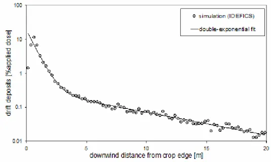
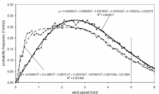
(31) RIVM report 607407002. The runs resulted in 20 datasets of drift deposition (percentage of areic mass applied) versus distance from the treated crop. Double exponential functions {a1exp(b1x)+a2exp(b2x)} were fitted to the data to reduce the computational effort for the further scenario selection. The fits of the double exponential curves were considered acceptable in view of the scenario selection. Figure 8 shows an example. Note that the vertical axis has a logarithmic scale. A maximum wind speed of 5 m s-1 was used, because above this wind speed spray application is not allowed in the Netherlands (except in rare crop-threatening situations).. Figure 8 Downwind deposits of spray drift for an application in a potato crop using a 50% drift-reducing (DG11004) nozzle in a cross-wind with an average speed of 3 m s-1. Dose is defined as mass per area (areic mass).. 4.2. Impact of wind speed, wind angle and ditch dimensions Wind speed varies from day to day and also across the day. As wind speed affects the spray drift deposition on surface water, the distribution of wind speed over time should be taken into account when deriving the 90th percentile concentrations in surface water resulting from spray drift. Figure 9 gives the frequency distribution of hourly average wind speeds over a period of ten years for the meteorological station Haarweg in Wageningen. Two distributions are given: (i) the distribution for all hourly average wind speeds, and (ii) the distribution for all hourly average wind speeds for the period between sunrise and sunset. The polynomial fitted through the second distribution was used for further calculations. The curve for the Haarweg location was used for the entire area of the Netherlands, because such detailed information was not readily available for each location in the Netherlands at the time of the selection. The period between sunrise and sunset was considered a good approximation of the period of the day where spray applications in the open field are possible or performed.. Page 30 of 129.

(32) RIVM report 607407002. Figure 9 Frequency distribution of hourly averaged wind speeds at 2 m height; ten-year averages for meteorological station ‘Haarweg’, Wageningen. Circles: distribution for natural day (24 h); triangles: distribution for daylight hours only. Dashed curve: polynomial fit for former distribution; bold curve: polynomial fit for latter distribution. The standard drift deposition curve is for the situation in which the wind direction is perpendicular to the ditch. For every other wind direction, drift droplets have to cover a longer distance from the point of release to the surface water. The additional distance is calculated from the width of the spray-free zone according to:  1  dadd  d   1  cos( )  . (1). where d (m) is the distance from the point of release to the deposition point when wind direction is perpendicular to the ditch, dadd (m) is the additional travel distance, and θ (rad) is the wind direction angle relative to a cross-wind (perpendicular) direction. On the other hand, the stretch over which a substance may be deposited on the surface water is also greater. The increase may be calculated with the same formula, taking the width of the surface water as input:  1  wadd  w   1  cos() . (2). where w (m) is the width of the surface water, and wadd (m) is the additional length over which spray drift may be deposited. The average drift deposition on surface water over width x is the integral of the deposition over width x divided by this width. It turns out that the deposition per square m surface water decreases with increasing wind direction angle, see Figure 10. At angles above 90°, droplets are not moving towards the ditch and drift deposition is zero.. Page 31 of 129.

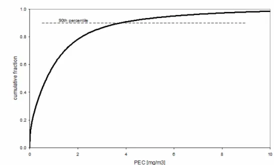
(33) RIVM report 607407002. Figure 10 Example of drift deposition on surface water as a function of wind direction (relative to perpendicular). Dose is defined as mass per area (areic mass). As described in Section 3.2, ditches in the Netherlands can be categorised into 66 classes, each defined by their width and depth. If the water level in the ditch is known and it is assumed that drift deposited on the water is immediately homogeneously distributed over the entire volume of water, then the initial peak concentration in the surface water can be calculated. For the scenario selection, water depth was assumed to be at ‘normal water level’ (see Chapter 6). The peak concentration is then equal to the average mass deposited per surface area divided by the average water depth. As described earlier, we decided to use the peak concentration for the selection of the scenarios.. 4.3. Selection of the scenario for downward spraying The combination of 66 ditch profiles, 35 wind directions and 20 wind speeds gives a total number of 46,200 different situations, each with its own peak concentration in the water. Figure 11 gives the cumulative frequency distribution of all these peak concentrations.. Page 32 of 129.

(34) RIVM report 607407002. Figure 11 Cumulative frequency distribution of all possible peak concentrations in surface water The selection of a realistic worst case condition (i.e. the 90th percentile) requires that weights be assigned to the possible peak concentrations. This was done as follows:  Certain types of ditch are more abundant than others, so weights have to be attributed to the abundance of ditch types. For each of the 66 ditch classes the abundance is known for each grid cell of 1 km2 in terms of total length and total volume. Because we are interested in the assessment of effects on aquatic organisms, the length of the ditches was used as a weighting factor.  The management decision (see Section 2.1) that a ditch should potentially receive both drift and drainage from artificial drains, limits the population of ditches to only those ditches that are in artificially drained areas. A map of areas that are drained is shown in Figure 2 and this information was used in the selection. So ditches outside the drained areas were assigned a weight of zero.  Primary, secondary and tertiary ditches may all be edge-of-field ditches. There is no information on the proportion of each ditch type being edge-offield ditches, so this aspect could not be taken into account during the selection. This implies that no weight was attached to the type of ditch. Notice, however, that primary ditches do generally not receive input from drainpipes; this group of ditches is therefore implicitly eliminated from the population.  For the total population of ditches, it was assumed that there is no preferred angle between the ditch and the wind direction, so each angle has equal chance to occur and thus there is no weighting due to angle. Although there is a main wind direction in the Netherlands, this assumption is considered valid because we have no evidence for a preferred direction of ditches in the Netherlands.. Page 33 of 129.

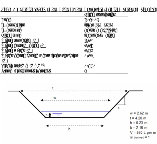
(35) RIVM report 607407002. Peak concentrations, weighted according to the procedure above, were plotted in a contour diagram (Figure 12). The X-coordinate in this diagram corresponds with the percentile of the cumulative spatial distribution (resulting from ditch properties) and the Y-coordinate with the cumulative distribution due to variability of weather conditions (wind speed and wind angle). The figure indicates that several combinations of wind characteristics and ditch characteristics may lead to the same peak concentration. For example, the points X=80 per cent, Y=80 per cent and X=60 per cent, Y=97 per cent both yield an overall percentile of 90 per cent.. Figure 12 Contour diagram of percentiles of weighted concentrations. The horizontal axis arranges the ditches on their average concentration whereas the vertical axis arranges the effects of wind speed and direction. The lines in the diagram have equal probability of occurrence. The diagram is limited to ditches in drained areas in the Netherlands. The endpoint for the exposure assessment is the 90th overall percentile, so a combination of water body type, wind speed and wind direction should be chosen from the contour line labelled 90. As there are many possibilities, further selection was necessary. Criteria for further selection were:  The combination should be within 3 per cent of the target value (so between the 87th and 93rd percentile).  The wind speed should be between 3.25 and 3.5 m s-1.  The wind angle should be within 10 o of perpendicular.  The ditch should be a ditch that is found in areas where land use is predominantly arable.  The ditch should be a tertiary or a secondary ditch, because primary ditches usually do not receive input from drains. The final selection was based on expert judgement, taking into account the relative abundance of field crops. Preference was given to a ditch that is typical for the region where the drainpipe scenario is located, as this would yield a coherent scenario. Table 2 and Figure 13 give the most important characteristics of the selected ditch.. Page 34 of 129.

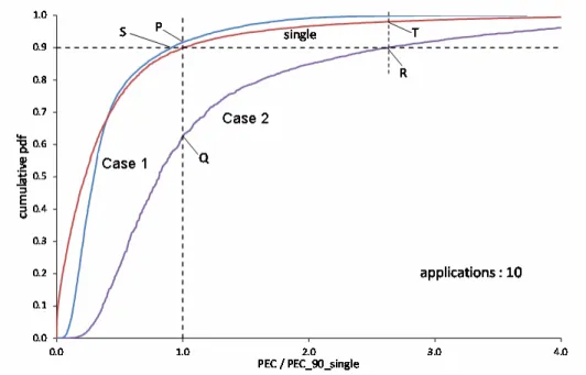
(36) RIVM report 607407002. Table 2 Characteristics of the ditch for the downward-directed spraying scenario Ditch properties Code 601001 Hydroregion river clay area Hydrotype Betuwe backland Ditch type secondary ditch Width top ditch (m) 4.20 Width bottom ditch (m) 2.16 Width water (m) 2.62 Water depth at the wet-winter situation 0.23 (m) Lineic volume (m3 m-1) 0.550 Slope (horizontal:vertical) 1. Figure 13 Dimensions of the ditch for the downward-directed spraying scenario (code 601001), where w is the width of the water surface, h is the water depth, b is the width of the bottom of the ditch, t is the width of the top of the ditch, s1 is the side slope (horizontal/vertical), and V is the lineic volume of the water in the ditch.. 4.4. Multiple applications The spray drift scenario selection was based on a single application. In practice, several treatments during the growing season are common. Van de Zande et al. (2012) performed Monte Carlo simulations to investigate whether the selected spray drift scenario is also appropriate for multiple applications. Two extreme cases were investigated, i.e.: 1. The concentration in the surface water does not decrease after an application within a growing season, so the PEC caused by subsequent applications within a growing season builds up. 2. The concentration in the surface water decreases to zero between subsequent applications. The Monte Carlo simulations were performed as follows. For each of the 66 standard ditches, 500 ‘events’ were simulated in which an event is defined as a set of ten repeated applications within a single growing season. One event results in a single PEC value, because the maximum concentration within a year has to be taken. The total number of results was 33,000. These results were plotted in a cumulative frequency distribution and compared with the frequency distribution resulting from a single application (Figure 14).. Page 35 of 129.

(37) RIVM report 607407002. Figure 14 Cumulative probability density function (pdf) showing PEC values (relative to PEC90 of a single application) for ten spray applications. Red curve: cumulative pdf for single application; blue curve: for case 1 after ten applications; purple curve: for case 2 after ten applications. Points P, Q, R, S and T: see text. The red line is the frequency distribution resulting from a single annual application and corresponds to the frequency distribution plotted in Figure 11. The frequency distribution for case 1 (the case in which the concentration builds up) is slightly steeper than the frequency distribution resulting from a single application, which implies that the frequency distribution resulting from multiple applications shows less variability. This was expected, because within a year, applications may be carried out under favourable or unfavourable weather conditions. This has an averaging effect on the final PEC, because only this final PEC is used for generating the frequency distribution. The 90th percentile of the PEC resulting from case 1 (point S) is about 10 per cent lower than the 90th percentile resulting from a single application. Also, the 90th percentile of the concentration distribution for the single application corresponds to a higher percentile of the concentration distribution for case 1 (about 92nd percentile: point P). It can therefore be concluded that the spray drift scenario based on a single application is only slightly too conservative for case 1. In case 2, the frequency distribution has shifted towards a larger (relative) value (purple line). Also in this case, individual applications within a year vary because of different wind conditions. However, in this case the concentration drops to zero after an application and the maximum annual concentration is determined only by the most unfavourable application. As a result, the 90th percentile of the concentration distribution for case 2 (point R) is much higher (by almost a factor of three) than the 90th percentile concentration resulting from a single application, so the scenario based on a single application may generate a PEC value that is much too low for case 2 (the 90th percentile concentration for the single applications corresponds only to the 60th percentile of the concentration distribution for the multiple application, point Q).. Page 36 of 129.

(38) RIVM report 607407002. The above findings indicate that the scenario based on single applications may not be sufficiently conservative for multiple applications. This can be solved by taking a higher percentile of the concentration distribution resulting from single applications. In case 2, for example, the 98th percentile of the concentration distribution resulting from a single application would have to be selected (point T). As it is to be expected that an even higher percentile needs to be selected if more than ten applications within a growing season are simulated, this results in an extremely conservative scenario for single applications and for case 1. We therefore recommend developing a procedure in which the percentile to be selected depends on the number of applications and the type of substance. Note that the findings reported here are different from those described in FOCUS (2001). First, FOCUS considered only case 1 (where a shift towards a less conservative percentile occurs) and not case 2 (where a shift towards a more conservative percentile occurs). Second, FOCUS (2001) assumed a normal distribution of wind speed and wind direction for a single spray drift event and considered only a single surface water system. We simulated the ensemble population of 66 surface water systems using a uniform distribution of the wind angle and a distribution of the wind speed based on hourly values during daytime taken from weather station in Wageningen. Thus we consider our simulations more realistic. Figure 14 shows that our curve for the single event deviates strongly from a normal distribution (it can probably be described better with a lognormal distribution).. 4.5. Conclusions A systematic procedure was followed in order to select a ditch covering realistic worst case conditions with respect to exposure from downward-directed drift deposition. The selection resulted in a number of possibilities. Application of additional plausibility criteria reduced the number of ditches chosen to one. The selected ditch is a secondary water course typical of river clay areas with a water width of 2.6 m, a water depth of 0.23 m, and a lineic volume of 0.550 m3 m-1 (code 601001). It should be noted that this is the water depth at the so-called wet winter situation (Massop et al. 2006). The selection was based on a single application. It was shown that this scenario may not be sufficiently conservative for multiple applications, particularly if the concentration does not build up between subsequent applications within a growing season. We therefore recommend developing a procedure in which the percentile to be selected depends on the number of applications within a growing season and the type of substance.. Page 37 of 129.


(40) RIVM report 607407002. 5. Selection of the drainpipe scenario. This chapter summarises the selection of the drainpipe scenario to be included in the exposure scenario for field crops and downward spraying. A more detailed description can be found in Tiktak et al. (2012b). The aim of the study reported in this chapter was to parameterise a drainpipe exposure model for realistic worst case conditions. Realistic worst- case conditions are defined as the 90th percentile of all ditches that potentially receive PPPs from drainpipes. Here, the population of ditches is not limited to ditches that receive both a spray input and a drainpipe input, because there is no relationship between wind direction and drainpipe orientation.. 5.1. Approach Drainpipe exposure is calculated with a new version of the pesticide fate model PEARL (Tiktak et al. 2012a, 2012c). A new version of PEARL was necessary, because the version that is currently used in authorisation procedures (Leistra et al. 2001) does not include a description of preferential flow through macropores. Preferential flow is considered to be the key driver for the peak concentration in drain water. Central in the new model is a description of the geometry of macropores and the presence of a so-called internal catchment domain. This internal catchment domain consists of macropores that end above drain depth (Figure 15).. Figure 15 Schematic representation of the two macropore domains, i.e. the main bypass flow domain, which transports water deep into the soil profile, possibly leading to rapid drainage, and the internal catchment domain, in which infiltrated water is trapped in the unsaturated soil matrix at different depths. PEARL was applied to the Andelst experimental field site (Section 5.2). Soil and hydrological data from this field site were the basis for the drainpipe scenario. The advantage of using data from this site is that full benefit could be taken of the experimental data, so that a consistent and credible drainpipe scenario could be build. The dataset covers one year of data. The working group decided, Page 39 of 129.

No results found