PBL Working Paper 7 / CPB Discussion Paper 220
October 2012
Air Pollution Policy in Europe: Quantifying the Interaction with
Greenhouse Gases and Climate Change Policies
*Johannes Bollen§, Corjan Brink#
CPB Netherlands Bureau for Economic Policy Analysis, The Hague, The Netherlands PBL Netherlands Environmental Assessment Agency, The Hague, The Netherlands
Abstract
This paper uses the computable general equilibrium model WorldScan to analyse
interactions between EU’s air pollution and climate change policies. Covering the entire world and seven EU countries, WorldScan simulates economic growth in a neo-classical recursive dynamic framework, including emissions and abatement of greenhouse gases (CO2, N2O and
CH4) and air pollutants (SO2, NOx, NH3 and PM2.5). Abatement includes the possibility of
using end-of-pipe control options that remove pollutants without affecting the emission-producing activity itself. This paper analyses several variants of EU’s air pollution policies for the year 2020. Air pollution policy will depend on end-of-pipe controls for not more than 50%, thus also at least 50% of the required emission reduction will come from changes in the use of energy through efficiency improvements, fuel switching and other structural changes in the economy. Greenhouse gas emissions thereby decrease, which renders
climate change policies less costly. Our results show that carbon prices will fall, but not more than 33%, although they could drop to zero when the EU agrees on a more stringent air pollution policy.
JEL Classification: Q53, Q54, Q42, D58, H21
Keywords: air pollution, climate change, energy, co-benefits, interaction policies
* The authors would like to thank Herman Vollebergh for his valuable comments on an earlier version of this paper as well as Stefan Boeters for his comments and suggestions regarding the setup of the model. Their input significantly improved the quality of the analysis presented in this paper.
§ CPB, Telephone: +31 70 3383319, e-mail: J.C.Bollen@cpb.nl # PBL, Telephone: +31 30 2743639, e-mail: Corjan.Brink@pbl.nl
1
Introduction
Emissions of greenhouse gases (GHGs) and air pollutants originate from fossil fuel
combustion. Mitigating the emissions of carbon dioxide (CO2) requires changes in the fuel
mix and savings on the use of fossil fuels. These structural changes also reduce emissions of air pollutants. But, ‘end-of-pipe’ (EOP) options, i.e. control technologies lowering emissions without affecting the emission-producing activity itself - are considered to reduce air
pollution more cost-effectively. In the past, air policies in Europe have relied mainly on these EOP options, and not surprisingly there was a negligible effect of these policies on the GHG emissions. For this reason, air policies are considered to have little or no impact on climate policies. On the other hand, it is widely recognized that policies aimed at reducing GHG emissions yield co-benefits in reducing emissions of air pollutants (Rive, 2010; Burtraw et al., 2003; Syri et al., 2001). Hence, it may not come as a surprise that the European Commission decided to postpone the revision of reduction targets for air pollutants in order to first account for the outcome of their climate policy plans.
In the past decades in Europe, especially the low-cost EOP abatement options have been exploited to mainly mitigate acidification. More recently, pollution policy is broadened with the more restrictive issue of human health (EC, 2005; EC, 2011). Consequently, structural changes - although expensive - may become part of an efficient policy package. In this paper we use a multi-sector, multi-region, global Computable General Equilibrium (CGE) model including the possibility of EOP abatement to analyse the relevance of structural changes in optimal (welfare-maximising) emission reduction strategies for air pollutants. Indeed, we find that a cost-effective reduction consists of structural changes in the economy and energy markets. These changes go hand in hand with co-benefits of lower GHG
emissions from large point sources within the Emission Trading System (ETS) and small point sources in the other producing sectors and households (non-ETS). Disregarding
structural changes when thinking about new targets for emissions of air pollutants, may lead to sub-optimal allocation of emission reductions over Member States. Moreover, as reducing air pollution yields air pollution benefits at a local scale in the near future, in contrast with the avoided climate damages of GHG mitigation which are at a global scale in the distant future, this is an argument to incite the European Commission to establish new air policy targets prior to further elaborating climate policy plans.
To our knowledge there are hardly any CGE studies on air pollution policies in Europe that fully integrate EOP abatement for a considerable number of air pollutants and structural changes in a consistent economic framework. The bottom-up study of Amann et al. (2008) show the cost-effectiveness of structural measures, such as energy efficiency improvements, in reducing air pollution health impacts in China. But they do not consider non-technical changes in the economy, such as a reallocation of resources towards production sectors that are less energy-intensive or a shift to energy-extensive consumption. Bollen et al. (2009a,b) and Bollen et al. (2010) consider local air pollution and global climate change policies in an intertemporal cost-benefit analysis, accounting for the value of reduced air pollution and climate change. They find that structural changes contribute to air pollutant mitigation, not only in China and India, but also in the OECD (Bollen et al. 2009b). Their analysis however lacks details with respect to sectors and countries within the EU.
Only Rive (2010) integrates EOP emission control options of air pollutants in a CGE model of the EU. But he limits to a static model analysis of the year 2020, one aggregate EU
region, one of the Kyoto gases (CO2) and air pollution only from large stationary energy
sources (which is only half of the air pollution problem). Our paper is in line with Rive (2010), but more comprehensive in several aspects. With respect to climate policies, our approach is broader as we model all emission categories and all known abatement options of the non-CO2 GHGs. With respect to air pollution, we not only model emissions of the air
pollutants of sulphur (SO2), nitrogen (NOx) and particulate matter (PM), but also enrich the
analysis by modelling emissions and abatement of ammonia (NH3). Moreover, in this paper
we cover all emission categories by also including emissions and abatement of small point and mobile sources and in our baseline we consider as well air pollution control according to emission control legislation already laid down in national laws. Finally, we disaggregate EU-27 to seven countries and two aggregate regions, as we want to analyse national air
pollution targets with the location of emissions being relevant for their impact on health and ecosystems.
Summarizing, our analysis adds to the literature as this paper covers the most relevant air pollutants and GHG emissions in recursive dynamic framework. We will show to what extent emission reductions can be obtained by structural changes in the economy as well as by EOP measures. Data on emissions and EOP abatement were derived from the GAINS model, which includes a detailed representation of technological options for abatement of GHGs and air pollutants (Wagner and Amman, 2009; Amann et al., 2011).
Section 2 describes WorldScan, the model used for our analyses, focussing on the
extensions of the model with respect to earlier applications of the model. Section 3 presents the policy cases considered. The main results of the simulations appear in section 4. Then, section 5 discusses the interactions between air and climate policies, within the context of the next steps in climate and a policy considered in the EU policymaking process, and concludes.
2
WorldScan
2.1 Overview
The macro-economic consequences of specific climate or air policy scenarios are assessed using the global applied general equilibrium model WorldScan. A detailed description of the model is given in Lejour et al. (2006). Here we give only a brief sketch of the main
characteristics of the model as it has been used for various kinds of analyses with respect to climate policies (see Bollen et al., 2004; Wobst et al., 2007; Manders and Veenendaal, 2008; Boeters and Koornneef, 2011; and Bollen et al., 2011). Extensions of the model necessary to analyse interactions between air and climate policies will be described more elaborately. These relate to the introduction of emissions of air pollutants and non-CO2 GHGs
and the representation of EOP emission control in the model.
WorldScan data for the base year 2004 were, for the most part, taken from the GTAP-7 database (Badri and Walmsley, 2008), which provides integrated data on bilateral trade flows and input-output accounts for 57 sectors and 113 countries and regions. The
aggregation of regions and sectors can be flexibly adjusted in WorldScan. The version used here features 23 regions and 18 sectors, listed in Table 1. Regional disaggregation is
relatively fine within Europe, but coarse outside. The main reason is that in Europe, policies for air pollution are materialised in terms of emission ceilings for air pollutants that are country specific because of regional differences in the impacts of air pollution on human
health and ecosystems. Moreover, the costs and the potential of emission control options may differ significantly between countries. The set of sectors reasonably represents the heterogeneous characteristics of activities causing emissions of GHGs and air pollutants. A distinction is made between sectors taking part in the EU emission trading system (ETS, consisting of the electricity and the energy-intensive sector) and sectors that do not participate in the emission trading system and households1 (NETS). Coal , oil and natural
gas are the primary energy sectors.2
WorldScan is set up to simulate deviations from a “Business-As-Usual” (BAU) path by imposing specific additional policy measures such as taxes or restrictions on emissions. The BAU used here is not generated by WorldScan itself, but calibrated on the Reference
Scenario of the World Energy Outlook 2009 (WEO-2009) as implemented in the GAINS model. For the EU member states, the Baseline 2009 scenario was used that has been developed with the PRIMES model for the European Commission (PRIMES-2009; Capros et al., 2010). Basic inputs for the baseline calibration are time series for population and GDP by region, energy use by region and energy carrier, and world fossil fuel prices by energy carrier. Appendix A describes in more detail the calibration of the BAU.
The electricity sector is refined with a detailed electricity technology specification developed by Boeters and Koornneef (2011). Electricity generation technologies are represented by linearly increasing supply functions and are calibrated using existing estimates of cost ranges and potentials. WorldScan captures five concrete electricity technologies: (1) fossil electricity, (2) wind (onshore and offshore) and solar energy, (3) biomass, (4) nuclear energy and (5) conventional hydropower. The BAU is calibrated to reproduce the shares of these technologies in total electricity production in each region as in WEO-2009 and PRIMES-2009. In our policy scenarios the quantities of wind and biomass endogenously react assuming increasing supply functions, while nuclear and hydropower are kept at their BAU levels (as in Boeters and Koornneef, 2011).
<<<Table 1 around here >>>
2.2 Modelling pollutant emissions and end-of-pipe abatement
To deal with the interaction between air and climate policies, WorldScan needs to cover not only the most relevant anthropogenic emissions of GHGs (CO2, CH4 and N2O), but also major
air pollutants. To this end, the model was extended to include emissions of sulphur dioxide (SO2), nitrogen oxides (NOx), fine particulate matter (PM2.5), and ammonia (NH3).3
1 A concordance matrix is used to relate aggregate production sectors to well-known aggregated consumption categories. These final consumption categories include: [1] Food, beverages and
tobacco, [2] Clothing and furniture, [3] Gross rent and fuel, [4] Other household outlays, [5] Education and medical care, [6] Transport and communication, [7] Recreation, and [8] Other goods and services consumed (see Lejour et al., 2006).
2 The sector Oil delivers mainly to Petroleum and coal products, which in turn delivers fuels to various sectors (in particular the transport sectors) and to households.
3 Although VOC emissions have an impact on health through ozone formation, we disregard VOC in this paper. Ozone contributes less to detrimental health effects than particulate matter. Moreover, it
concerns a global air pollutant, which implies that other regions also contribute to Europeans’ exposure to ozone. Finally, VOC emissions are mainly non-energy related, so the interactions with climate change policies are expected to be small.
Basic principles of emissions and emission abatement
CO2 emissions can be calculated easily in a CGE model because CO2 is emitted in fixed
proportions to the volume of fossil fuels burned, depending only on the fuel used. This is not true for emissions of other pollutants, such as SO2 and NOx, for which the level of emissions
depends on characteristics of the fuel combustion processes. Moreover, part of the emissions of these pollutants are not related to fossil fuel combustion, but are caused by, e.g.,
agricultural activities and waste disposal. A distinction can be made between emissions that are directly related to a specific input to production (such as fossil energy) and those
inherent to the production process, independent of the inputs. These ‘process emissions’ can be related to the output level of a sector.
Generally, emission reductions can be achieved in various ways. At the macro-level, Copeland and Taylor (2004) distinguish reductions through the scale effect (related to a reduction in the size of the economy as a whole), through the composition effect (resulting from a reallocation of resources in the economy towards less polluting sectors), and through the technique effect (by a reduction in the emission intensity within production sectors). A reduction in emission intensity in a sector can be achieved by technical change (leading to a more efficient use of inputs such as fossil fuels), substitution across different inputs (such as a switch from coal to natural gas) and application of emission control technologies (such as purification of exhaust gases).
Applied modelling efforts that study the economic consequences of climate policy
strategies can be classified into two broad categories of modelling approaches: (i) ‘bottom-up’ models, and (ii) ‘top-down’ models (Markandya et al., 2001; Vollebergh and Kemfert, 2005). Bottom-up models generally feature a large number of discrete energy technologies to capture substitution of energy carriers on the primary and final energy level, process substitution, or efficiency improvements (Böhringer and Rutherford, 2008). Top-down (such as CGE) models, adopt an economy-wide perspective and provide a stylized representation of the whole economy and its underlying structure built around behavioural assumptions of both investment and consumption. Whereas bottom-up models are suitable for a
disaggregated analysis of technologies that can be applied to reduce the emission intensity of certain economic activities (technique effect), CGE models have their strength when it comes to structural changes (i.e. the scale and composition effect).
Approaches to include emission control in a CGE framework
The literature provides several approaches for including emission control in a CGE model. The general concept is that actors can choose between paying for emissions and investing in pollution control. Pollution control can be considered as non-productive inputs reducing pollutant emissions at a certain cost. The approaches differ in the way in which the
abatement costs are incorporated in the model. Hyman et al. (2002) introduce emissions as an input to the production function, placed at the top of the nested production structure. The elasticity of substitution between the emissions and the conventional inputs is estimated to match a Marginal Abatement Cost (MAC) curve that is derived from detailed bottom-up studies (see Hyman et al., 2002; Reilly et al. 2002). Gerlagh et al. (2002) and Dellink et al. (2004) introduce for each pollutant an abatement sector producing mitigation technologies in a region. Emission reductions can be achieved by increasing the input of abatement goods in the production of a polluting sector, which allows for an abatement-specific input mix. The
elasticity of substitution between emissions and abatement is estimated to fit the data on abatement cost of options in a specific sector as available from various data sources. Rive (2010) included abatement in a CGE model by source-specific technology steps, each step representing groupings of abatement technologies with similar marginal abatement costs. This offers a flexible treatment that can incorporate activity- and pollution-specific marginal abatement cost curves of different shapes from bottom-up studies.
Emissions in WorldScan
In WorldScan, emissions are introduced at different places of the nested production
structure. Emissions from energy use are calculated using a fixed emission coefficient (i.e. a fixed amount of emissions per unit of coal, oil, natural gas, or biomass used).4 The use of
chemical fertilizer in agriculture is a significant source of emissions of N2O and NH3. As
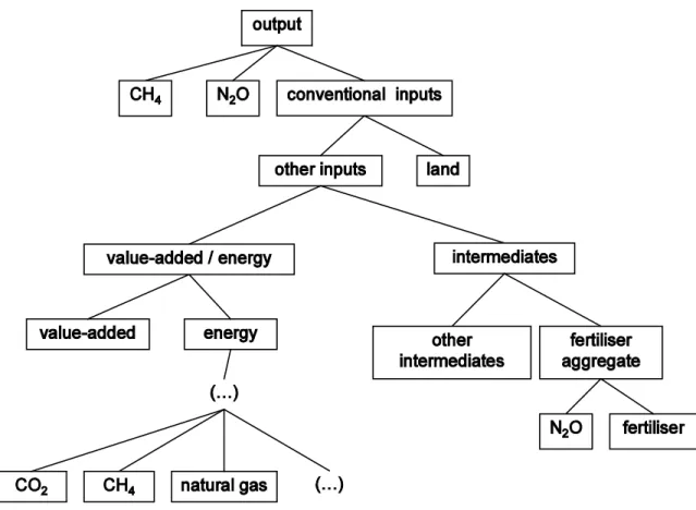
chemical fertilizer use is not included as a separate input in the GTAP database, in WorldScan emissions related to the use of chemical fertilizer are calculated using the intermediary input from the chemical sector to the agricultural sector as a proxy for the amount of fertilizer used. This is illustrated by the nesting of the production function in Figure 1. Emissions that cannot directly be linked to a particular input into the production process are included in the model as process emissions (they are thus linked to the sectoral output, the top of the production function nest).
For CO2, the emission factor linking emissions to energy use differs per fuel type but is
independent of the sector and region. Emission factors for other substances may also differ between sectors and regions. To take these differences into account, emission factors for non-CO2 GHGs and air pollutants in WorldScan are calculated such that emission levels by
region, sector and activity in the BAU reproduce the corresponding emission levels as calculated by the GAINS model.5 Hence, the country-, sector- and activity-specific emission
factors in WorldScan incorporate detailed information on emission sources as included in the GAINS model. This also includes emission control that is assumed to be implemented in the BAU induced by existing legislation (Amann et al., 2011).6 In a policy scenario, the emission
coefficient is fixed to the BAU level. In general, emissions of a particular pollutant by sector s can be represented by the following expression:
, , ,
s i s i s Q s s i
UEM
=
∑
ε
q
+
ε
Q
(1)With
UEMs
the level of emissions without emission control,qi,s
the volume of inputi
used in production of sectors
(such as fossil fuels and chemical fertilizer), εi,s the emissions per
4 This is a simplification in the model as in reality; emission coefficients are not necessarily fixed. For example, SO2 emissions per unit of oil depend on the sulfur content of oil. Oil in WorldScan, however, represents an aggregate for different types of oil. Therefore, the emission factor represents the average emission rate for oil in the BAU. The option of reducing emissions by a shift to oil with a lower sulfur content is included in the marginal abatement cost curves as described below.
5 We assume a mapping between GAINS sectors and WorldScan sectors as described in Appendix B. 6 The control options of GAINS are mapped to WorldScan sectors in the same was as emissions, and the options are ranked according to marginal costs. Thus, a MAC curve is constructed for each WorldScan sector (and input per sector) if the options exist in GAINS if that applies to that particular sector and input.
unit of this input used, and
εQ,s
the emission factor for process emissions by sectors
, i.e. the emissions per unit of sectoral outputQs
.<<< Figure 1 around here>>> Emission control in WorldScan
Changes in the volume of inputs
qi,s
and of outputQs
will change the emission levels. In addition, WorldScan introduces the possibility to invest in emission control. The model includes abatement supply curves for each type of emission (input-related and process) in each sector. Emission control reduces the level of emissions as they would occur without additional emission control below the BAU level:(
1
,)
, ,(
1
,)
,s i s i s i s Q s Q s s i
EM
=
∑
−
x
ε
q
+ −
x
ε
Q
(2)with
xi,s
andxQ,s
the relative abatement level due to emission control applied to input-related emissions and output-input-related emissions respectively. The supply function foremission control in this sector (i.e. the marginal abatement cost curve) represents the cost of abatement per unit of emissions which depends on the relative abatement level x. This function reads as follows (omitting indices for region-sector-activity-substance specifics):
(
)
( )
i ii
c x
β
x x
−χγ
δ
p
=
⋅
−
−
⋅
∑
(3)c(x)
gives the marginal cost of abatement as a function ofx
,x
is the maximum share of emissions that can be reduced by emission control options,β
andχ
are parameters (both > 0) which determine the curvature of the supply function, andγ
is a constant that determines the initial level of the marginal costc(0)
. Emission control requires the inputs of energy, capital, labour, intermediate goods and services. Parameterδi
indicates the share of inputi
in the total inputs required. As the abatement supply curves represent an aggregate of various emission control options with each different input requirement, it is not feasible to derive an appropriate input structure for each region-, sector-, activity-, and substance-specific curve. Instead, the parameters
δi
are set equal to the input shares of the capital goods sector in the respective region in the base year.7 Changes in the price of inputs,pi
,have an impact on the marginal cost of abatement. For example, if wages rise, the marginal cost of abatement will also increase, proportional to the share of labour in production.
Integration of the marginal abatement cost function gives the total abatement cost function:
( )
1(
)
11
s i i iC x UEM
β
x
χx x
χγ
x
δ
p
χ
− −
=
⋅
−
−
−
⋅
−
∑
(4)7 As emission control measures will in many cases be capital goods, on average the production and implementation of these measures will be similar to that of capital goods.
A tax on emissions will give producers an incentive to reduce pollution, either by structural changes or by EOP abatement.8 As can be shown EOP is applied up to the level where
marginal abatement cost by EOP equals the tax on emissions. Both investment in EOP and the emission tax to be paid for remaining emissions leads to additional production cost. As polluting activities become more expensive, substitution will lead to a decreasing share of the polluting inputs in production. Moreover, overall production costs increase depending on the emission intensity and the abatement cost, but also depending on the share of the polluting input in total production cost and the elasticity of substitution between the polluting input and other inputs. The increase in production cost will lead to an increase in the price of the product, which causes a shift within the economy from products with a high emission intensity and relatively expensive abatement towards products associated with less pollution related cost.
The functional form of the abatement supply curve is selected because of its flexibility, in order to be able to approximate a range of MAC curves as obtained from external sources. Marginal cost of abatement become infinitely large for levels of
x close to x
. For the analysis here, the values of the parametersx
,β
,χ
,γ
, andδi
were estimated from a set of marginal abatement cost curves from the GAINS model, including for each region-sector-activity-substance combination those mitigation options that are available in addition to those options GAINS assumes to be implemented in the BAU in 2020 (Amman et al., 2011). Abatement is expressed as a share of the emission level, rather than in absolute amounts, to take into account an increasing (decreasing) abatement potential in case of an increase (decrease) of the polluting activity due to changes in production structure or output levels. Using sector-specific abatement supply makes it possible to take into account differences between sectors with regard to the possibilities and costs of reducing emissions. This is of particular interest if environmental policies are differentiating between sectors—such as is the case in the EU, where climate policy sets different targets for sectors within ETS and NETS.By using equation (3) for expressing MAC curves in WorldScan, we can deal with a wide domain of abatement for many emission sources without an excessive computational burden. Hence, the model produces a numerical decomposition of abatement into EOP and structural changes. The approach applied by Rive (2010), approximating detailed MAC curves by several technology steps with constant marginal cost, offers more flexibility in representing MAC curves of different shapes. Nevertheless, we consider our approach adequate to analyse the trade-off between EOP and structural changes.
3
Policy cases
We assess interactions between air and climate policies analyzing several policy cases with different sets of emission reduction targets for GHGs and air pollutants up to the year 2020. A vital element of the EU’s air policy is the National Emission Ceilings (NEC) Directive, which sets upper limits for each Member State for total emissions of air pollutants. These ceilings are country-specific as they take into account regional differences in the impact of air
8 Appendix D derives the mathematical expressions for the optimal end-of-pipe abatement level for a given emission price in a simple analytical model, and provides information on how EOP is
pollution on human health and ecosystems and differences in the cost and potential of air pollutant mitigation (Wagner et al., 2010). A revision of the NEC Directive will establish emission ceilings for SO2, NOx, PM, Volatile Organic Compounds (VOC) and NH3, which have
to be met by Member States in 2020.
The EU’s climate policy was laid down in the EU Climate Change and Energy Package, which sets climate and energy targets for 2020: (i) a reduction in EU GHG emissions by 20% below 1990 levels, (ii) 20% of EU energy consumption to come from renewable sources, and (iii) a 20% reduction in primary energy use compared with projected levels through
improved energy efficiency. More specific, the Package sets an EU-wide cap on GHG emissions from sectors within the Emission Trading System (ETS) and binding national reduction targets for emissions from households and sectors not covered by the ETS (NETS). Member States are allowed flexibility in meeting their NETS targets, for instance by
transferring part of their annual emission allocation for a given year to other Member States.9 The targets relate to the aggregated emissions of the most relevant GHGs.10
Given the restrictions on emissions implemented in the policy cases, WorldScan is used to determine emission prices that are sufficiently high to reduce emissions to these targets. The emission prices reflect the marginal cost of abatement. Because of differences in reduction targets, prices of air pollutants vary between substances and regions. For GHGs, emission prices are equal for different substances, according to their CO2-equivalent weight.
Moreover, emission prices will be equalized between EU Member States due to the possibility of emission trading, resulting in an EU-wide price for emissions from sectors within ETS and one for emissions from NETS.
<<<Table 2 around here>>
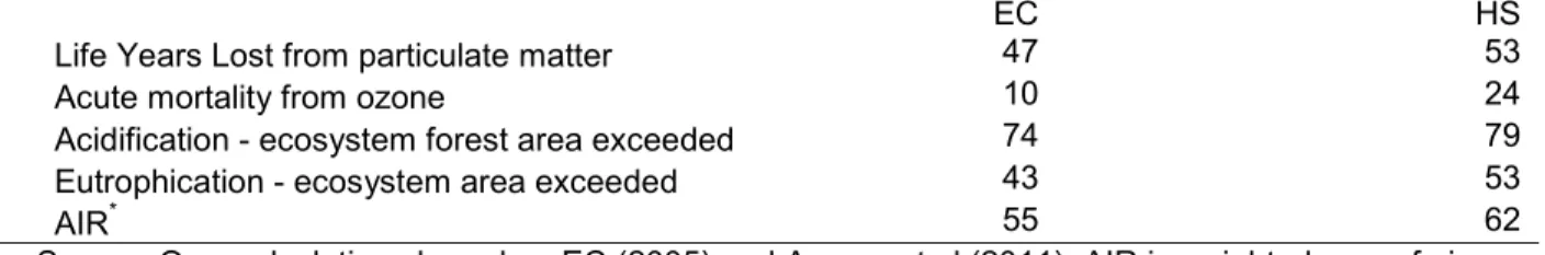
We analyze two variants of air pollution policies, covering the broad range of ambition levels for reducing air pollution impacts that have been considered in the decision-making process towards the revision of the EU NEC Directive so far. One is referred to as EC and reflects the objectives the European Commission has established in its Thematic Strategy on Air Pollution (EC, 2005). The other is referred to as HS and is based on the case with the highest ambition level as considered in the negotiations on the revision of the Gothenburg Protocol (i.e. the ‘High*’ case in Amann et al. 2011). Table 2 presents the respective relative improvements in health and ecosystem indicators. To convert the environmental objectives to appropriate country- and substance-specific emission targets in WorldScan, we used the outcome of optimization runs by the GAINS model that determined sets of emission
reductions for air pollutants in each country that achieve the EU-wide environmental objectives at least cost. We used emission levels for the TSAP case in Wagner et al. (2010) as emission ceilings in our CE variant. The optimization runs by the GAINS model take into account atmospheric transport of emissions, differences between countries in abatement potential and cost, and geographical differences in impacts of air pollution on human health
9 Flexibility is subject to certain conditions, as laid down in the ‘Effort Sharing Decision’, Articles 3.2, 3.4 and 3.5.
10 ETS currently covers only CO
2 emissions, but will be extended to include other GHGs, such as N2O from chemical industry. NETS covers CO2, N2O, CH4 and several F-gases. F-gases are not included in this analysis, because they have limited interaction with air pollution. Emissions of different GHGs are added up by converting them to CO2-equivalents according to their Global Warming Potential (CO2: 1; N2O: 310; CH4: 21).
and ecosystems (Wagner et al., 2007). This explains why percentage emission reductions required in the different policy variants widely differ between countries. To summarize the emission levels of the air pollutants in our cases, Table 2 presents a weighted sum of emissions of SO2, NOx, NH3 and PM2.5.11
The variants for air policies are combined with different variants for climate policies. Although the EU’s Climate Change and Energy Package has already been promoted to legislation, to examine the full impact of air policies on GHG emissions we constructed theoretical policy cases of “clean” air policy variants in which EU countries are subject to emission ceilings for air pollutants without having to reduce any GHGs. In addition, CC includes targets for GHG emission reductions in accordance with the EU Climate Change and Energy Package.12 Annex I countries outside the EU are assumed to meet the lower end of
the range of reduction targets they pledged under the Copenhagen Accord of December 2009.13
4
Results
We use WorldScan to assess the impact of the policy cases described above. This section presents results for 2020, with a particular focus on country-specific emissions,
decomposition of emissions to activities and sectors, and on prices and welfare. Welfare changes are measured by the Hicksian Equivalent Variation (HEV), i.e. the additional income required to compensate for any losses of utility with respect to the baseline without any policies, see also Boeters and Kornneef (2011), and Bollen et al. (2011). Any change in environmental quality is not included in this indicator. Section 4.1 investigates the
importance of structural changes induced by air policies. In general, we analyze impacts of policies by comparing simulations of scenarios with and without policies. Section 4.2 introduces climate policies next to air policies, to analyze the interaction between air pollution and climate policies.
4.1 Co-benefits of air policies
Here we present results of policy cases simulating EU-27 countries imposing national emission ceilings for air pollutants in a world without any climate policies. This scenario is useful to illustrate the extent to which air policies alone may provoke structural changes in EU-27 economies, and indirectly leads to co-benefits of lower GHG emissions.
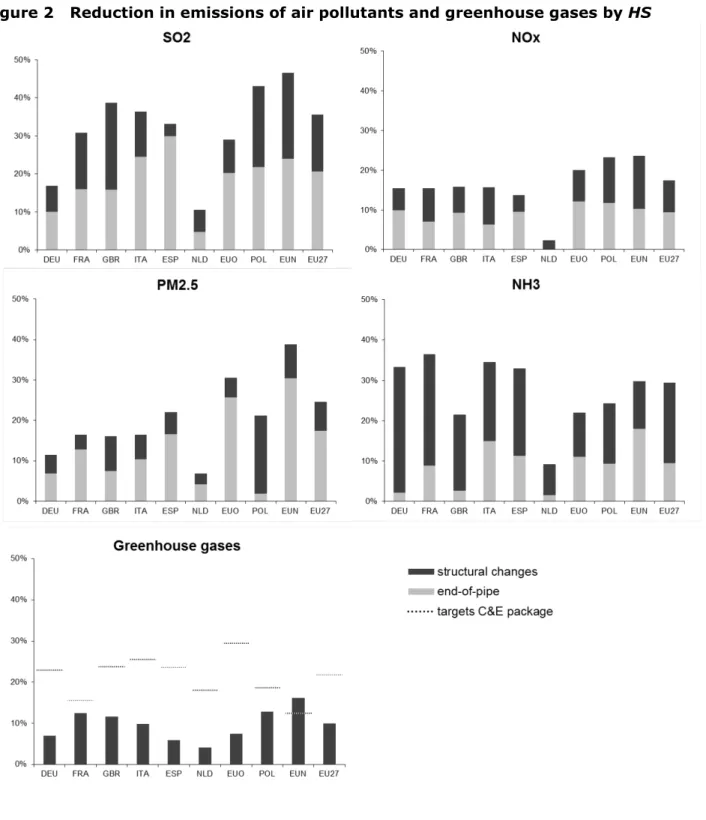
Figure 2 presents the emission reduction in the HS variant in all EU countries/regions distinguished in WorldScan, as well as for the EU-27. The emission reductions are presented for all air pollutants and for GHG’s. The contribution of EOP abatement to achieve this reduction is also illustrated. It can be seen that in the HS variant - on average in the EU - the contribution of EOP abatement to total emission reductions of SO2, NOx, PM2.5 and NH3
are equal to 58%, 54%, 71% and 32% respectively. The remaining part of the emission reductions result from structural changes within the EU economy, incited by the prices to be
11 Weights are based on the relative contribution of emissions of SO
2, NOx, PM2.5 and NH3 in the different EU member states to particulate matter exposure in the EU-27.
12 The GHG emission reduction in 2020 is equal to 20% of the 1990 emission level. The use of CDM is excluded.
13 Pledged targets are presented at
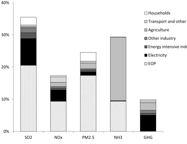
paid for air pollutant emissions. Figure 3 decomposes the impact of structural changes in EU-27 on emissions to sectors.
<<<Figure 2 around here>>>
From Figure 3 it can be seen that in the power sector about 20% of the total emission reduction of SO2 and NOx relates to structural change. The structural changes in the power
sector originate mainly from a changing fuel mix, electric demand savings leading to decreasing production levels, and efficiency improvements within the power sector. In the agricultural sector, structural changes are even more pronounced, and account for about two thirds of the total NH3 emission reduction. The emissions price of NH3 significantly increases
the costs of production in the agricultural sector, and leads to reallocation of production and pollution to other countries without any air pollution policy. The decline in production in EU-27 also lowers the emissions of NOx and PM2.5.
The importance of EOP controls in emission reduction is country-specific as the stringency of the emission target and the shape of marginal cost curves of EOP is country-specific. For example, for SO2 a relatively large share of EOP is observed in Spain, Rest of EU15 and Italy
due to a relatively large abatement potential of low-cost EOP abatement in the energy intensive sectors, petroleum and coal products and coal-fired power plants. For NH3, EOP
contributes less to abatement in Germany, the UK and the Netherlands because of relatively high EOP control costs.
<<<Figure 3 around here>>>
The indirect impact of GHG emission abatement only results from structural changes induced by the air policies, because – by assumption – there is no incentive for any EOP mitigation related to GHG’s. Overall, EU-27 GHG emissions decrease by 10% with respect to BAU, 50% of which is related to from a decrease in the use of coal in favour of natural gas and efficiency improvements in fossil electricity generation. About 25% of the GHG emission reduction originates from NH3 emission targets in the agricultural sector, which leads to
competitiveness and production losses in this sector, and indirectly lowers the emissions of CH4 and N2O.
Figure 2 also indicates the GHG emission reduction targets of the EU Climate and Energy package as a percentage reduction with respect to BAU. This shows that overall, almost 50% of the reduction in GHG emissions as required under the EU Climate and Energy package will be achieved as a co-benefit of this HS air pollution policy scenario. More specifically, this percentage is equal to 35% of the ETS reduction effort and 81% the NETS reduction effort in the EU-27.
Rive (2010) estimates the contribution of structural change of SO2 emissions reduction to
be 25% (in a scenario without climate policy). This is somewhat less than the 42% we find for SO2. A major difference between our analysis and Rive (2010) is on the BAU
assumptions. Whereas Rive (2010) adopts a BAU in which emission factors are kept constant at base year levels (i.e. no additional technologies are implemented), our BAU follows the PRIMES-2009 baseline as implemented in the GAINS model, assuming air pollution control according to emission control legislation already described in national laws. This implies that, contrary to Rive’s analysis, in our analysis most of the ‘low-hanging fruit’ of EOP abatement
is not available anymore in our policy simulations, thus leaving Europe with more expensive reduction options, including structural changes.
4.2 Interaction air pollution and climate change policies
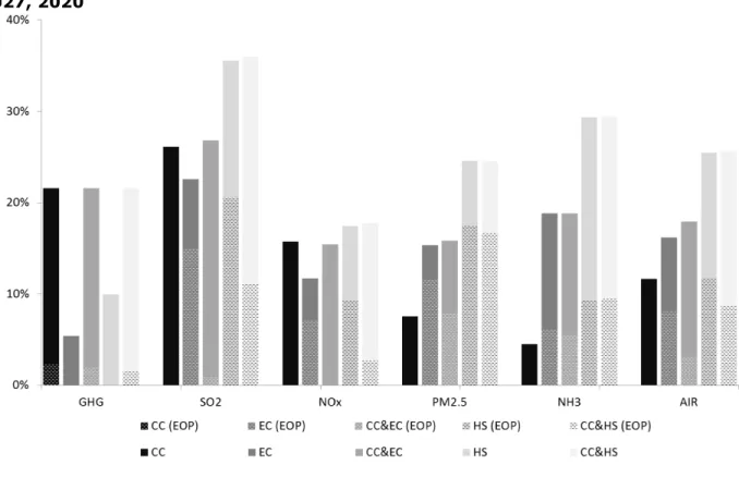
The previous section argued that structural changes in the economy unfold because of air pollution policies. This section analyzes air pollution policies in combination with climate change policies. Figure 4 presents the reduction in emissions of GHGs and air pollutants from the climate change policy scenario CC and two policy scenario that combine the assumptions of CC with air pollutant targets of EC and HS.
<<<Figure 4 around here>>>
The CC scenario yields a 22% reduction in GHG emissions, 90% of which results from structural changes. The structural changes yield also reductions in emissions of air pollutants, in particular SO2 (26%) and NOx (16%). This co-benefit from climate change
policies are the ones often presented in the literature, like Criqui et al. (2003) and van Vuuren et al. (2006). Typically, these co-benefits come from a decreasing share of fossil energy, efficiency improvements, and electricity savings. Reductions in PM2.5 and NH3
emissions are smaller (8% and 4% respectively). PM2.5 reductions result from changes in the
electricity production, but also from a lower demand for residential heating. NH3 emissions
decrease from production losses in the agricultural sector, which are driven by mitigation of non-CO2 gases. The co-benefits (SO2 and NOx) are large enough to push emissions below the
EC ceilings, except for Spain and Poland. As for emissions of PM2.5, they decrease below the
EC ceilings only in the UK and Poland. NH3 emissions in all countries remain above EC
ceilings.
Introduction of air pollution targets in addition to climate policies will change the efficient allocation of GHG mitigation over EU member states. In CC&EC, the efforts to meet the air pollution targets have an effect on the GHG emission trade between countries. As emissions of air pollutants are partly reduced by structural changes in the economy, emissions of GHGs simultaneously decrease. Consequently, the demand for GHG emission permits will decrease while at the same time the supply of permits will increase. This is in particular the case for the non-ETS sectors, where demand decreases by 8 Mton CO2-equivalents while supply
increases by 10 Mton CO2-eq., resulting in a lower price of GHG emissions by non-ETS
sectors (€10/ton CO2-eq. compared to €15/ton CO2-eq. for CC). The ETS price remains
nearly unaffected at €30/ton CO2-eq. as in ETS sectors additional reductions of air pollutant
emissions are mainly obtained by EOP and GHG emissions are hardly affected. With more ambitious air pollution policies (CC&HS), effects are more pronounced. Reductions in emissions of air pollutants cause a further decrease in GHG emissions in several member states. In Italy, the demand for permits by ETS sectors will decrease by 4 Mton CO2-eq. whereas in Rest of EU-27 and France the supply of permits by ETS sectors will
increase by 9 and 5 Mton CO2-eq. respectively, causing the ETS price of GHG emissions to
decrease to €28/ton CO2-eq. For emissions by non-ETS sectors, both in Germany and Spain
demand will decrease by 5 Mton CO2-eq. while at the same time supply of emission
reduction by France and Italy will increase by 17 and 4 Mton CO2-eq. respectively, which
the interaction between different endogenous emission prices take effect in the model, Appendix C presents a detailed elaboration of the impacts in several cases for the coal-fired power plants in the new member state countries (excluding Poland) of the EU-27.
In the EU-27, the introduction of air policies causes an increase in the contribution of the agricultural sector to the total GHG emission reductions in the NETS sectors from 26% in CC to 40% (CC&EC) and 48% (CC&HS). This has its origin - like in the earlier presented HS scenario - in the relatively large contribution of structural changes in the agricultural sector induced by the reduction targets for NH3, which also have an impact on CH4 and N2O
emissions, of which agricultural activities are an important source.
Figure 4 not only presents the reduction in emissions of the individual air pollutants, but also the reduction in the sum of emissions of SO2, NOx, NH3 and PM2.5 weighted to their
contribution to particulate matter exposure in the EU-27, referred to as AIR. This aggregate serves as a rough indicator for the change in health impact in the EU resulting from the reduction in emissions of air pollutants (see OECD, 2012). The reduction in emissions of AIR from climate policies (CC) amounts to 72% of the reduction obtained with the EC variant, and to 46% with the HS variant. Recall that the EC variant reflects the objectives of the European Commission in its Thematic Strategy on Air Pollution. Conversely, the air pollution policy variants EC and HS yield 25% and 46% of the overall reduction in GHG emissions aimed for in the Climate and Energy package of the EU. Generally, it can be seen that air pollution policy will depend on end-of-pipe controls for not more than 50% (the share of EOP contributing to reduction in the EC variant), thus also at least 50% of the required emission reduction will come from changes in the use of energy through efficiency improvements, fuel switching and other structural changes in the economy.
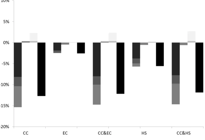
Finally, Figure 5 presents the changes in primary energy use in EU-27 resulting from climate policy (CC), air pollution policies (EC and HS) and a combination of these (CC&EC and CC&HS). Primary energy use is split up in the use of the fossil fuels coal, oil, and natural gas, the non-fossil energy carriers biomass, nuclear and other renewables (wind, sun and hydropower). Biomass is presented separately from the other renewables as on the one hand it is applied as an option to mitigate CO2 emissions, but on the other hand the use of
biomass is a source of air pollutant emissions. <<<Figure 5 around here>>>
The figure confirms the insight that seeking only to achieve air targets without pursuing any climate policy goals will already restructure the economy of the EU-27. The response is to switch away from fossil fuels, mainly coal, and save on energy by 3-6% of total primary energy use (EC and HS variant). Reductions in coal (electricity) are mainly driven by the SO2
target, reductions in oil (transport) by the NOx and PM2.5 targets, and reductions in gas
(mainly electricity) by the NOx targets. The increase of non-fossil energy demand is limited
as energy saving seems to be cheaper and dominates the impacts on energy markets, see also Boeters and Koornneef (2011). Whereas climate policies without air policies lead to an increase in the use of bio-energy, this seems less attractive in the presence of reduction targets for air pollutants because using biomass for energy purposes results in emissions of air pollutants. Remarkably, the reduction in primary energy use is less in CC&HS than in CC, in spite of the additional price to be paid for emissions of air pollutants. This results from agricultural production losses of stringent NH3 targets as part of the air pollution policy,
which also lowers the emissions and the price of GHG, and hence dampens savings on primary energy use.
Finally, it can be seen that in all variants the use of coal decreases most, because the burning of coal burning is more emission intensive than of oil or natural gas. But - in the variants including climate policy - the use of natural gas is affected more than the use of oil, although on average per unit of energy used oil emits more GHGs than natural gas. The reason is that in the EU, pre-existing energy taxes are generally higher for oil than for natural gas. Consequently, the effect of additional emission prices on end-user prices is relatively smaller for oil and so is the impact on demand.
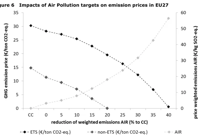
<<<Figure 6 around here>>>
As described above, GHG emission prices decrease when air pollution policies are
introduced. This is particularly the case for the non-ETS emission price because of the effect of the NH3 reduction target on the agricultural sector and hence on agricultural emissions of
(non-CO2) GHGs. Figure 6 shows the impact of air policies on GHG emission prices for ETS
and non-ETS markets. To simulate an increasing stringency of targets for air pollution taking into account differences in the impact on human health for different pollutants emitted at different locations, we apply an increasing reduction target for the weighted sum of emissions of air pollutants AIR (as described earlier). In these simulations, WorldScan determined the efficient allocation of emission reductions over pollutants and regions given the different weights of these pollutants in the various EU member states14.
With increasing reduction targets for AIR, the price on emissions of air pollutants
increases, thereby more and more replacing the taxes required to achieve the climate policy targets. The GHG emission price for non-ETS sectors drops to 0 €/ t CO2 eq with a reduction
of the weighted sum of air pollutant emissions of 20%. At this level of reduction in AIR the GHG emission price for ETS sectors drops to 20 €/ton CO2-eq. Targets to further reduce AIR
will further bring down the ETS price. For reductions of AIR by 40% or higher, ETS as an instrument of climate policy even becomes obsolete. This doesn’t mean that GHG emissions are not reduced, but the primary incentive for GHG emission reduction is not a price on GHG emissions but a price on emissions of air pollutants, which drives a decrease in electricity production (mainly coal).15 Moreover, the demand for electricity goes down because of the
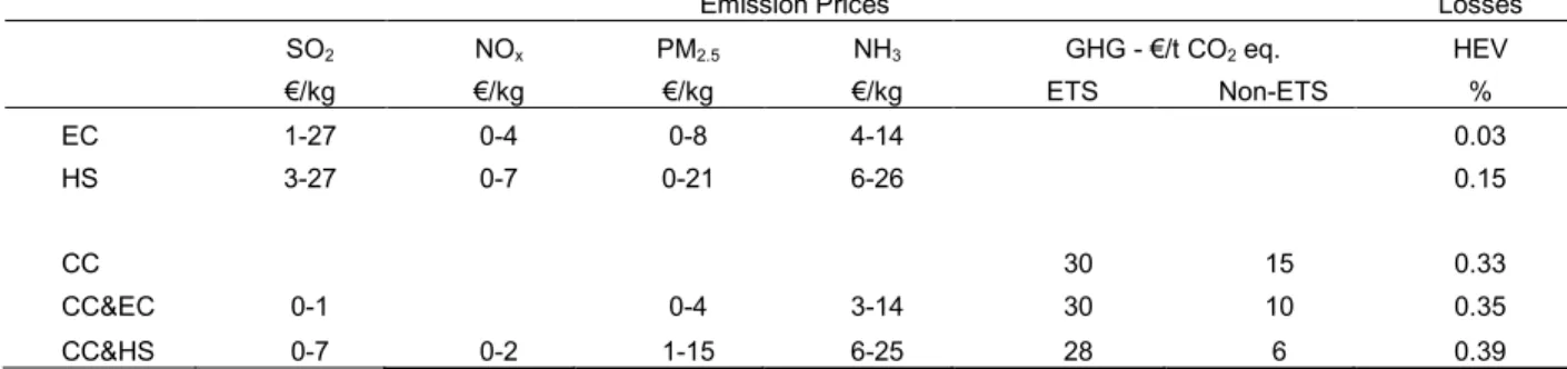
effect of air pollution policies on other sectors in the EU economies. <<<Table 3 around here>>
Finally, we summarize in Table 3 the economic impacts in 2020 in EU-27 of different policy variants by showing the emission prices related to the different substances and the welfare losses. The costs of the policy interventions are modest to small at the macro-level, i.e.
14 Note that the weights used for this indicator AIR are based only on the health effects of air pollutants. The effects of air pollutants on ecosystems through eutrophication and acidification are therefore not considered in this analysis of the relation between GHG emission price and stringency of air policies, while they were considered in the analysis with the GAINS model to determine the
emission ceilings used for the EC and HS variants. As a result, reduction of NH3 emissions, which have a relatively large effect on eutrophication, is less substantial.
15 See also a detailed example of coal-fired powerplants in New Member States (excluding Poland) in Appendix C.
welfare losses increase up to 0.39% of BAU national income at the most. The climate policy scenario CC already accounts for a 0.33% welfare loss. Whether there are climate policies or not, the welfare effects of the air policy variants are smaller than those related to climate change. Without climate policies, air pollution targets result in a welfare loss of 0.03-0.15%. With existing climate policies, additional welfare losses due to targets for reducing air
pollution are smaller, 0.02-0.06% point above the CC welfare losses. Notwithstanding the introduction of an additional distortion in a second-best economy, losses are smaller due to the synergy of structural changes simultaneously reducing emissions of GHGs and air pollutants. The distortion of the economy by air pollution is determined by the emission prices of different substances. Emission prices for air pollutants are country-specific, because of the country-specific emission targets. Table 3 shows the range of these prices in the EU-27. For greenhouse gases, two carbon prices exist, one for ETS and one for non-ETS
emissions. We already highlighted the effect of air pollution policies on GHG emission prices, especially in the non-ETS sectors. The main reason is that stringent ammonia targets lead to a substantial cost increase for the agricultural sector, resulting in a reallocation of production of this sector to countries outside the EU-27. Consequently, non-CO2 gases from the
agricultural sector (i.e. non-ETS) will decline. . Vice versa, it can be seen that emission prices in sulphur decline when carbon prices are introduced, resulting from a switch towards more carbon extensive fuels (e.g. from coal to gas or renewable energy). Also prices for NOx
and PM2.5 are affected by carbon prices, especially the NOx price going down to zero in the
CC&EC variant compared to EC scenario. The reduction of the PM2.5 emission price - when
introducing climate policy - is smaller compared to the change in NOx and SO2 prices. The
main reason is that the use of biomass for energy purposes is stimulated because of climate policy, but biomass burning leads to emissions of PM2.5. Nevertheless, decarbonising the
energy mix results in a net reduction in PM2.5 emissions. Finally, ammonia prices are less
sensitive to climate policy, because agriculture is energy extensive and abatement of non-CO2 gases constitutes a small part of total GHG abatement.
Summarizing, when air targets become more binding, carbon prices will decrease, but not more than 33%, although they could drop to zero when the EU agrees on a much more stringent air pollution policy. Welfare losses depend on the stringency of the air target, and those of the air policies analysed in this paper are lower than those of the climate change policy options, especially if analysed in addition to the current climate policies.
5
Discussion
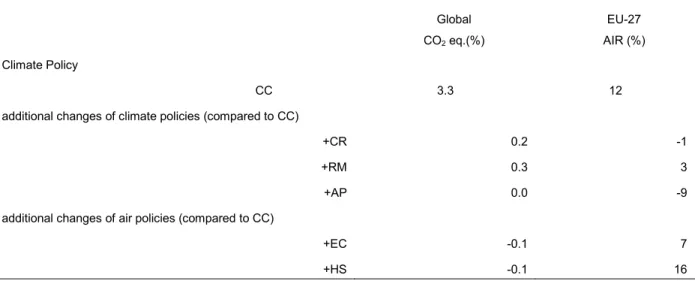
The previous section demonstrated the potential impact of air pollution policies on GHG emissions and hence on climate policies. To assess the welfare effects of the interaction between air and climate policies for alternative climate policies that are considered or implemented in the EU, this section presents the main results of simulations representing additional targets and possible next steps of the EU in mitigating climate change. We briefly assess the simulation results for 2020, and focus on the weighted sum of air pollutant
emissions (AIR) in the EU and global CO2-equivalent emissions, which are presented in Table
4. The latter variable is included to indicate the order of magnitude of the benefits to Europe of reduced global warming. The AIR emission reduction is included as an indication for health benefits in Europe from avoiding air pollution.
We introduce three additional climate policy variants representing more ambitious
mitigation targets for GHG mitigation than in the CC case presented earlier in Section 4. The CR variant adds a 20% target for renewable energy in the EU in addition to the assumptions of the CC case. The RM variant assumes a 25% emission reduction in GHG emissions below 1990 levels in 2020, which is in line with the EU Energy Roadmap 2050, while mitigation efforts in the rest of the world are the same as in CC. The AP variant, on the other hand, assumes Annex I countries to meet the higher (stringent) end of the range of reduction targets they pledged under the Copenhagen Accord of December 2009. For the EU, this implies a reduction in GHG emissions by 30% below 1990 levels. Moreover, China and India are assumed to meet their pledged targets of lowering their CO2 intensity compared to 2005
with 45% and 25%, respectively. This AP variant also assumes international emission trading between Annex I countries, leading to a uniform price for GHG emissions in these countries.
The CR variant assumes a subsidy on renewable energy to push its share to 20% in 2020 (compared to 13% in CC). Within fossil electric markets, the share of coal will increase at the expense of gas, with, total emissions within ETS remaining constant. An increase in the demand for coal in the EU will lead to higher global prices of coal, reducing the demand for coal outside the EU. Hence global CO2 emissions will fall. At the same time, the subsidy on
renewable energy will cause an increase in the use of bio-energy. As biomass burning results in PM2.5 emissions, this will push emission levels of AIR. The renewable energy policy causes
welfare losses to increase by 50% compared with CC (i.e. from 0.33% to 0.5%).
The RM scenario assumes a further reduction of EU-27 GHG emissions to 25% below 1990 emission level. The extra emission reduction compared with CC translates to a 0.3 %
reduction of global GHG emissions16. Compared with CC, the reduction in energy use in RM
will result in a 3% extra emission reduction of AIR. Welfare losses increase by another 0.1% point.
More complicated is the AP scenario, in which the EU reduction targets are increased to 30% below the 1990 emission levels. The AP scenario, however, also includes emission trading between the EU-27 and other abating countries and as the EU will buy emission permits from other countries, GHG emissions within the EU-27 will increase compared to the CC case. Emissions are traded at 8 €/tCO2, which is much lower than the EU emission prices
of 30 €/tCO2 (ETS) and €15/tCO2 (non-ETS) in the CC case). Despite the increased
stringency of the overall target of most member states of the climate coalition, the impact on global GHG emissions Is negligible. The reason is that Russia and the Ukraine will sell their large surplus of emission rights (hot air), hence increasing the overall emissions of abating countries. The EU will achieve a higher welfare level (0.3% compared to the BAU), resulting from terms-of-trade gains.
<<<Table 4 around here >>>
As presented before, the variants combining GHG mitigation targets with air pollution policies, CC&EC and CC&HS, will call for extra reductions of NH3 emissions by the
agricultural sector. Hence, NH3 emissions will be taxed which causes the cost of agricultural
production to increase. As a consequence, production will be partly reallocated to regions
16 This includes carbon leakage to regions without reduction targets, mainly resulting from decreasing global fuel prices (Boeters and Bollen, 2012)
that have no air pollution policies. An increase of agricultural production in these countries will result in an increase of associated CH4 and N2O emissions. This explains the slight
increase in global GHG emissions in CC&EC and CC&HS compared to CC. This leakage of GHG emissions causes the GHG leakage rate to increase from 20% in CC to 24% in
CC&HS.17 Air quality improves as AIR emissions are reduced by 7 and 13% compared the CC
case in the CC&EC and CC&HS scenarios, respectively. Welfare losses are limited, especially in the CC&EC case.
Summarizing, all simulations (including those addressing climate change) show small impacts on global GHG emissions, indicating that the benefits of reduced climate change will be limited in these scenarios. Climate policies result in reductions in emissions of air
pollutants as a co-benefit, but introducing a target for renewable energy share in CR leads to a small reduction of these co-benefits. An international climate agreement accompanied by emission trading between Annex I countries will substantially reduce these co-benefits as the EU will reduce less emissions domestically and instead buy emission permits from other Annex I countries. The RM variant, however, shows an increase in the co-benefits to air pollution. Thus, any next step of the EU in either air or climate policy involves a small change in global GHG emissions, and a significant impact on EU’s emissions of AIR. While keeping in mind that the avoided damages from climate change are small and will occur in the far future compared to avoided damages of air pollution that will be significant for EU citizens in the next decade - the most favorable step in EU environmental policy making seems to hint on mitigating air pollution as opposed to climate policies. As argued in this paper, very stringent air pollution policies will provoke structural changes in the economy that will lower the GHG emissions as well. Still, the stringency of the air targets has to be decided, but has been beyond the scope of analysis of this paper.
This paper focussed on air policies in Europe, but the WorldScan model used has global coverage. Future work will investigate air pollution policies and their interaction with climate policies in non-EU regions as well. We expect that, in particular in China, air pollution
policies will impact fossil energy markets and prices, and hence may have an effect on other countries’ economies and environmental policies and global GHG emissions.
17 Here, the leakage rate is defined as the ratio between the reduction in GHG emissions within the EU-27 and the increase in emissions outside the EU-EU-27.
References
Amann,M., Kejun, J., Jiming, H., Wang, S., Xing, Z, Wei, W. Xiang, D.Y., Hong , L., Jia, X., Chuying, Z., Bertok, I., Borken, J., Cofala, J., Heyes, C., Höglund, L., Klimont, Z., Purohit, P., Rafaj, P., Schöpp, W., Toth, G., Wagner, F., and Winiwarter, W., 2008, GAINS-Asia. Scenarios for cost-effective control of air pollution and greenhouse gases in China, IIASA, Laxenburg, Austria.
Amann, M., Bertok, I., Borken-Kleefeld, J., Cofala, J., Heyes, C., Höglund Isaksson, L., Klimont, Z., Purohit, P., Rafaj, P., Schöpp, W., Toth, G., Wagner, F., Winiwarter, W., 2009. Potentials and Costs for Greenhouse Gas Mitigation in Annex I Countries:
Methodology. IIASA Interim Report IR-09-043 [November 2009], IIASA, Laxenburg, Austria.
Amann,M., Bertok, I., Borken-Kleefeld, J., Cofala, J., Heyes, C., Höglund Isaksson, L., Klimont, Z., Rafaj, P., Schöpp, W., Wagner, F., 2011. Cost-effective Emission Reductions to Improve Air Quality in Europe in 2020 - Scenarios for the Negotiations on the Revision of the Gothenburg Protocol under the Convention on Long-range Transboundary Air Pollution, CIAM2011-1 V2.1, IIASA, Laxenburg, Austria.
Badri, N.G., Walmsley, T.L., 2008. Global Trade, Assistance, and Production: The GTAP 7 Data Base, Center for Global Trade Analysis, Purdue University.
Boeters, S., Koornneef, J., 2011. Supply of Renewable Energy Sources and the Cost of EU Climate Policy, Energy Economics 33, 1024-1034.
Boeters, S., Bollen, J., 2012. Fossil Fuel Supply, Leakage and the Effectiveness of Border Measures in Climate Policy, Energy Economics, forthcoming.
Böhringer, C., Rutherford, T.F., 2008. Combining bottom-up and top-down, Energy Economics 30 (2), 574-596.
Bollen, J., Mulder , M., Manders, T., 2004. Four Futures for Energy Markets and Climate Change, Special Publication 52, CPB Netherlands Bureau for Economic Policy Analysis, The Hague.
Bollen, J., van der Zwaan, B., Brink, C., Eerens, H., 2009a. Local Air Pollution and Global Climate Change: A Combined Cost-Benefit Analysis, Resource and Energy Economics 31, 161-181.
Bollen, J., Guay, B., Jamet, S., Corfee-Morlot, J., 2009b. Co-benefits of Climate Change Mitigation Policies: Literature Review and New Results, OECD Economics Department Working Paper No. 693, OECD, Paris.
Bollen J., van der Zwaan, B., Hers, S., 2010. An Integrated Assessment of Climate Change, Air Pollution, and Energy Security Policy, Energy Policy 38, pp. 4021-4030.
Bollen, J., Koutstaal, P., Veenendaal, P., 2011. CPB Study Trade and Climate Change, 11 April 2011, EC, DG Trade, Brussels, Belgium,
http://trade.ec.europa.eu/doclib/docs/2011/may/tradoc_147906.pdf.
Burtraw, D., Krupnick, A., Palmer, K., Paul, A., Toman, M., Bloyd, C., 2003. Ancillary Benefits of Reduced Air Pollution in the US From Moderate Greenhouse Gas Mitigation
Policies in the Electricity Sector, Journal of Environmental Economics and Management 45, 650-673.
Capros, P., Mantzos, L., DeVita, N. Tasios, A., Kouvaritakis, N., 2010. Trends to 2030-update 2009,European Commission-Directorate General for Energy in collaboration with Climate Action DG and Mobility and Transport DG, August 2010. Office for official
publications of the European Communities, Luxembourg, ISBN 978-92-79-16191-9. Copeland, Brian R., Taylor, & M. Scott, 2004. Trade, Growth, and the Environment, Journal of Economic Literature, American Economic Association, vol. 42(1), pages 7-71, March.
Criqui, P., Kitous, A., Berk, M.M., den Elzen, M.G.J., Eickhout, B., Lucas, P., van Vuuren, D.P., Kouvarikatis, N., Van Regemorter, D., 2003). Greenhouse gas reduction pathways in the UNFCCC Process up to 2025. Technical Report, IEPE, Grenoble, see:
http://europa.eu.int/comm/environment/climat/pdf/pm_techreport2025.pdf.
Dellink R., Hofkes M., van Ierland E., Verbruggen H., 2004. Dynamic modelling of pollution abatement in a CGE framework. Economic Modelling 21, 965-989.
EC, 2005. Communication from the Commission to the Council and the European Parliament, Thematic Strategy on air pollution, SEC(2005) 1132 SEC(2005) 1133, COM(2005) 446 final, see also
http://eur-lex.europa.eu/LexUriServ/LexUriServ.do?uri=COM:2005:0446:FIN:EN:PDF.
EC, 2011. Commission Staff Working Paper on the Implementation of EU Air Quality Policy and Preparing for Its Comprehensive Review, SEC(2011) 342.
Gerlagh R., Dellink R., Hofkes M., Verbruggen H., 2002. A measure of sustainable national income for the Netherlands. Ecological Economics 41, 157-174.
Hyman R.C., Reilly J.M., Babiker, M.H., De Masin A., Jacoby H.D., 2002. Modeling non-CO2 greenhouse gas abatement. Environmental Modeling and Assessment 8, 175-186.
IEA (International Energy Agency), 2009. World Energy Outlook 2009, OECD/IEA.
Lejour, A.M., Veenendaal, P., Verweij, G., van Leeuwen, N., 2006. WorldScan: A Model for International Economic Policy Analysis, CPB Document 111, The Hague.
Manders T., Veenendaal, P., 2008. Border Tax Adjustments and the EU-ETS, A
Quantitative Assessment, CPB Discussion Paper 171, CPB Netherlands Bureau for Economic Policy Analysis.
Markandya, A., Mason, P., Perelet, R. and Taylor, T., 2001. A dictionary of environmental economics. London and India: Earthscan (London) and OUP (India).
OECD, 2012. The OECD Environmental Outlook to 2050: The Consequences of Inaction, OECD Publishing.
Reilly J, Mayer M, Harnisch J., 2002. The Kyoto Protocol and non-CO2 greenhouse gases and carbon sinks. Environmental Modeling and Assessment 7, 217-229.
Rive N., 2010. Climate policy in Western Europe and avoided costs of air pollution control. Economic Modelling 27; 103-115.
Vollebergh, H. R.J, Kemfert, C., 2005. The role of technological change for a sustainable development, Ecological Economics, Elsevier, vol. 54(2-3), pages 133-147, August.
van Vuuren, D.P., Cofala, J., Eerens, H.C., Oostenrijk, R., Heyes, C., Klimont, Z., den Elzen, M.G.J., Amann, M., 2006. Exploring the ancillary benefits of the Kyoto Protocol for air pollution in Europe. Energy Policy 34, 444–460.
Wagner, F., Amman, M., Schöpp, W., 2007. ‘The GAINS Optimization Module as of 1 February 2007, Interim Report IR-07-004, IIASA, Laxenburg, Austria.
Wagner, F., Amman, M., 2009). GAINS (Greenhouse gas - air pollution interactions and synergies): analysis of the proposals for GHG reductions in 2020 made by UNFCCC Annex 1 countries by mid-August 2009: IIASA, Laxenburg, Austria.
Wagner, F., Amann, M., Bertok, I, Cofala, J., Heyes, C., Klimont, Z., Rafaj, P., Schöpp, W., 2010. Baseline Emission Projections and Further Cost-effective Reductions of Air Pollution Impacts in Europe - A 2010 Perspective, NEC Scenario Analysis Report Nr. 6, IIASA, Vienna, Austria, http://www.iiasa.ac.at/rains/reports/
NEC7_Interim_report_20100827.pdf.
Wobst, P., Anger, N., Veenendaal, P., Alexeeva-Talebi, V., Boeters, S., van Leeuwen, N., Mennel, T., Oberndorfer ,U., Rojas-Romagoza, H., 2007. Competitiveness Effects of Trading Emissions and Fostering Technologies to Meet the EU Kyoto Targets: A Quantitative
Appendix A: Calibrating a BAU Scenario
The effects of climate policy depend strongly on the underlying BAU. The policy scenarios developed in this paper are based on the Reference Scenario of the 2009 World Energy Outlook (WEO-2009, IEA, 2009) and for the EU member states on the Baseline 2009 scenario developed with the PRIMES model as implemented in the GAINS model (PRIMES-2009, Capros et al., 2010). With our BAU, we deviate from the PRIMES-2009 scenario in one respect, however. We removed the ETS-caps to establish a level playing field in our
assessments of the mitigation pledges in an international context.
The BAU calibration employs trends for population and GDP by region, energy use by region and energy carrier, and world fossil fuel prices by energy carrier. Population is exogenous, but the other time series are reproduced by adjusting the model parameters. GDP is targeted by Total Factor Productivity (TFP, differentiated by sector), energy
quantities are targeted by energy efficiency, and fuel prices are targeted by the amount of natural resources available as input to fossil fuel production. In policy variants, TFP, energy efficiency, and natural sources are fixed, and GDP, energy use and prices are endogenous.
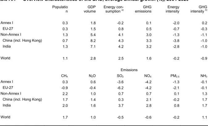
<<Table A.1 around here >>>
According to our BAU, the global population will continue to expand. Combined with worldwide economic growth of 2.7% per year, global demand for energy will be almost 30% higher in 2020 than in 2004. The effects of the financial and economic crisis are included in WEO-2009 and PRIMES-2009 and have a large impact on medium-term economic growth rates. The expansion of energy use predominantly takes place in Non-Annex I, thus partially reducing the gap in energy consumption per capita with the industrialized countries. Table A.1 gives some key overview characteristics of the baseline for the 2004-2020 period. The table indicates that energy- and GHG intensities are declining worldwide and especially in Non-Annex I. The BAU assumes the fossil fuel price projections of WEO2009 (e.g. the oil price will reach 100 US$ per barrel in 2020). In Europe, the gas price is expected to lag behind the oil price. Regional coal prices are expected to remain constant at their 2009 level.
Appendix B: Mapping from GAINS to GTAP 7
<<<here Table A.2>>>Appendix C: How EOP works in WorldScan: an example
Environmental policies are implemented in the model by introducing a price on emissions (Lejour et al., 2006). This emission price makes polluting activities more expensive, and provides an incentive to reduce these emissions. For emissions directly related to the use of a specific input, such as fossil fuels, the emission price in fact causes a rise in the user price of this input. Consequently, this leads to a fall in the demand for it and hence a reduction in emissions. For emissions related to sectoral output levels, the emission price causes a rise in the output price of the associated product. Consequently, this leads to a fall in demand for it and hence in a reduction in emissions. Moreover, if emission control options are available, these will be implemented up to the level where the marginal cost of emission control equals the emission price. The emission price can be introduced exogenously, but it is also possible to set a restriction on emissions in the model. In this case, the emission price is
endogenously determined in the model at the level needed to reduce emissions to the predetermined emission target.
<<<here Table A.3>>>
For illustrative purposes, we elaborate on the effect of a restriction on emissions of
greenhouse gases and on SO2 emissions for a specific sector, i.e. the coal-fired power plants
in the New Member States (excluding Poland). Table A.3 presents some relevant results for this sector in different scenarios on energy use, and for GHG and SO2 the prices of
emissions of, the resulting mark-up on the price of coal, the emissions, and the
decomposition of emission reductions in end-of-pipe and structural change. The scenarios illustrated in Table A.3 span the range of scenarios of focussing on only air pollution policies (HS), on only climate policy (CC), and on the combination of both climate and ambitious air policies (CC&HS) and the variant with even more stringent air pollution targets (CC&AIR-40), The latter scenario assumes an air pollution policy, which takes into account the differences in the impact on human health for different pollutants emitted at different locations, and applies a 40% reduction target for the weighted sum of emissions of air pollutants AIR. This aggregate AIR indicator serves as a rough indicator for the change in health impact in the EU resulting from the reduction in emissions of air pollutants, see OECD (2012).
In the baseline in 2020, the emissions of greenhouse gases and SO2 in the New Member States (excluding Poland) are equal to 192 Mton and 342 Kton, respectively.
The HS scenario sets emission ceilings for all air pollutants in EU-27 - 216 Kton SO2 -
leading to a price on sulphur emissions of €9.5/kg SO2-eq. This emission price increases the
price of coal with 60%, i.e. the user price of coal for coal-fired power plants in New Member states. Therefore, electricity becomes more expensive, and hence demand declines by 11%. Because SO2 emissions per energy unit are larger for coal than for oil and gas, the demand
for coal will fall more than proportionally: 33% (45-30=15 Mtoe). As a co-benefit of the air pollution policy, the emissions of GHG will be reduced (related to that specific activity also 33%).
Reductions in emissions of SO2 can also be achieved by end-of-pipe abatement. The